A model independent approach to non dissipative decoherence

Abstract

We consider the case when decoherence is due to the fluctuations of some classical variable or parameter of a system and not to its entanglement with the environment. Under few and quite general assumptions, we derive a model-independent formalism for this non-dissipative decoherence, and we apply it to explain the decoherence observed in some recent experiments in cavity QED and on trapped ions.

I Introduction

Decoherence is the rapid transformation of a pure linear superposition state into the corresponding statistical mixture

$$|\psi\rangle=\alpha|\psi_{1}\rangle+\beta|\psi_{2}\rangle\Rightarrow\rho_{mix}=|\alpha|^{2}|\psi_{1}\rangle\langle\psi_{1}|+|\beta|^{2}|\psi_{2}\rangle\langle\psi_{2}|\;;$$ (1)

this process does not preserve the purity of the state, that is, ${\rm Tr}\rho_{mix}^{2}<1$, and therefore it has to be described in terms of a non-unitary evolution. The most common approach is the so-called environment-induced decoherence [1, 2] which is based on the consideration that it is extremely difficult to isolate perfectly a system from uncontrollable degrees of freedom (the “environment”). The non-unitary evolution of the system of interest is obtained by considering the interaction with these uncontrolled degrees of freedom and tracing over them. In this approach, decoherence is caused by the entanglement of the two states of the superposition with two approximately orthogonal states of the environment $|E_{1}\rangle$ and $|E_{2}\rangle$

$$\left(\alpha|\psi_{1}\rangle+\beta|\psi_{2}\rangle\right)\otimes|E_{0}\rangle\Rightarrow|\psi\rangle_{TOT}=\alpha|\psi_{1}\rangle\otimes|E_{1}\rangle+\beta|\psi_{2}\rangle\otimes|E_{2}\rangle\;.$$ (2)

Tracing over the environment and using $\langle E_{1}|E_{2}\rangle\simeq 0$, one gets

$${\rm Tr}_{env}\left\{|\psi\rangle_{TOT}\langle\psi|\right\}=\rho_{mix}\;,$$ (3)

where $\rho_{mix}$ is defined in Eq. (1). The environment behaves as a measurement apparatus because the states $|E_{i}\rangle$ behave as “pointer states” associated with $|\psi_{i}\rangle$; in this way the environment acquires “information” on the system state and therefore decoherence is described as an irreversible flow of information from the system into the environment [1]. In this approach, the system energy is usually not conserved and the interaction with the environment also accounts for the irreversible thermalization of the system of interest. However this approach is inevitably model-dependent, because one has to assume a model Hamiltonian for the environment and the interaction between system and environment. This modelization, and therefore any quantitative prediction, becomes problematic whenever the environmental degrees of freedom responsible for decoherence are not easily recognizable.

Decoherence is not always necessarily due to the entanglement with an environment, but it may be due, as well, to the fluctuations of some classical parameter or internal variable of the system. This kind of decoherence is present even in isolated systems, where environment-induced decoherence has to be neglected. In these cases the system energy is conserved, and one has a different form of decoherence, which we shall call “non-dissipative decoherence”. In such cases, every single experimental run is characterized by the usual unitary evolution generated by the system Hamiltonian. However, definite statistical prediction are obtained only repeating the experiment many times and this is when decoherence takes place, because each run corresponds to a different random value or stochastic realization of the fluctuating classical variable. The experimental results correspond therefore to an average over these fluctuations and they will describe in general an effective non-unitary evolution.

In this paper we shall present a quite general theory of non-dissipative decoherence for isolated systems which can be applied for two different kinds of fluctuating variables or parameters: the case of a random evolution time and the case of a fluctuating Rabi frequency yielding a fluctuation of the Hamiltonian. In both cases one has random phases $e^{-iE_{n}t/\hbar}$ in the energy eigenstates basis that, once averaged over many experimental runs, lead to the decay of off-diagonal matrix elements of the density operator, while leaving the diagonal ones unchanged.

The outline of the paper is as follows. In Section II we shall derive the theory under general assumptions, following closely the original derivation presented in [3, 4]. In Section III we shall apply this theory in order to describe the decoherence effects observed in two cavity QED experiments performed in Paris, one describing Rabi oscillations associated with the resonant interaction between a Rydberg atom and a microwave cavity mode [5], and the second one a Ramsey interferometry experiment using a dispersive interaction between the cavity mode and the atom [6]. In Section IV we shall apply our approach to a Rabi oscillation experiment for trapped ions [7], and Section V is for concluding remarks.

II The general formalism

The formalism describing non-dissipative decoherence of isolated systems has been derived in [3, 4] by considering the case of a system with random evolution time. The evolution time may be random because of the finite time needed to prepare the initial state of the system, because of the randomness of the detection time, as well as many other reasons. For example, in cavity QED experiments, the evolution time is the interaction time, which is determined by the time of flight of the atoms within the cavity and this time can be random due to atomic velocity dispersion.

In these cases, the experimental observations are not described by the usual density matrix of the whole system $\rho(t)$, but by its time averaged counterpart [3, 4]

$$\bar{\rho}(t)=\int_{0}^{\infty}dt^{\prime}P(t,t^{\prime})\rho(t^{\prime})\;,$$ (4)

where $\rho(t^{\prime})=\exp\{-iLt^{\prime}\}\rho(0)$ is the usual unitarily evolved density operator from the initial state and $L\ldots=[H,\ldots]/\hbar$. Therefore $t^{\prime}$ denotes the random evolution time, while $t$ is a parameter describing the usual “clock” time. Using Eq. (4), one can write

$$\bar{\rho}(t)=V(t)\rho(0)\;,$$ (5)

where

$$V(t)=\int_{0}^{\infty}dt^{\prime}P(t,t^{\prime})e^{-iLt^{\prime}}$$ (6)

is the evolution operator for the averaged state of the system. Following Ref. [3, 4], we determine the function $P(t,t^{\prime})$ by imposing the following plausible conditions: i) $\bar{\rho}(t)$ must be a density operator, i.e. it must be self-adjoint, positive-definite, and with unit-trace. This leads to the condition that $P(t,t^{\prime})$ must be non-negative and normalized, i.e a probability density in $t^{\prime}$ so that Eq. (4) is a completely positive mapping. ii) $V(t)$ satisfies the semigroup property $V(t_{1}+t_{2})=V(t_{1})V(t_{2})$, with $t_{1},t_{2}\geq 0$.

The semigroup condition is satisfied by an exponential dependence on $t$

$$V(t)=\left\{V_{1}\right\}^{-t/\tau_{2}}\;,$$ (7)

where $\tau_{2}$ naturally appears as a scaling time. A solution satisfying all the conditions we have imposed can be found by separating $V_{1}$ in its hermitian and antihermitian part $V_{1}=A+iB$ and by considering the Gamma function integral identity [8]

$$(V_{1})^{-t/\tau_{2}}=\left(A+iB\right)^{-t/\tau_{2}}=\frac{1}{\Gamma\left(\frac{t}{\tau_{2}}\right)}\int_{0}^{\infty}d\lambda\lambda^{\frac{t}{\tau_{2}}-1}e^{-\lambda A}e^{-i\lambda B}\;.$$ (8)

Now the right hand side of Eq. (8) can be identified with the right hand side of Eq. (6) if we impose the following conditions: $\lambda=t^{\prime}/\tau_{1}$, where $\tau_{1}$ is another scaling time, generally different from $\tau_{2}$; $B=L\tau_{1}$ in order to make the exponential terms identical, and $A=1$ in order to get a normalized probability distribution $P(t,t^{\prime})$. This choice yields the following expressions for the evolution operator for the averaged density matrix $V(t)$ and for the probability density $P(t,t^{\prime},\tau_{1},\tau_{2})$ [3, 4]

$$V(t) = \left(1+iL\tau_{1}\right)^{-t/\tau_{2}}$$ (9)

$$P(t,t^{\prime},\tau_{1},\tau_{2}) = \frac{e^{-t^{\prime}/\tau_{1}}}{\tau_{1}}\frac{(t^{\prime}/\tau_{1})^{(t/\tau_{2})-1}}{\Gamma(t/\tau_{2})}\;.$$ (10)

Notice that the ordinary quantum evolution is recovered when $\tau_{1}=\tau_{2}=\tau\rightarrow 0$; in this limit $P(t,t^{\prime},\tau_{1},\tau_{2})\rightarrow\delta(t-t^{\prime})$ so that $\bar{\rho}(t)=\rho(t)$ and $V(t)=\exp\{-iLt\}$ is the usual unitary evolution. Moreover, it can be seen that Eq. (9) implies that $\bar{\rho}(t)$ satisfies a finite difference equation [3]. The semigroup condition leads to the form of the probability distribution $P(t,t^{\prime},\tau_{1},\tau_{2})$ we use to perform the average on the fluctuating evolution times. However, notice that this probability distribution depends on both the two scaling times $\tau_{1}$ and $\tau_{2}$ only apparently. In fact, if we change variable in the time integral, $t^{\prime\prime}=(\tau_{2}/\tau_{1})t^{\prime}$, it is possible to rewrite the integral expression for $V(t)$ in the following way

$$V(t)=\left(1+iL\tau_{1}\right)^{-t/\tau_{2}}=\int_{0}^{\infty}dt^{\prime\prime}P(t,t^{\prime\prime},\tau_{2})e^{-iL(\tau_{1}/\tau_{2})t^{\prime\prime}}\;,$$ (11)

where

$$P(t,t^{\prime\prime},\tau_{2})=\frac{e^{-t^{\prime\prime}/\tau_{2}}}{\tau_{2}}\frac{(t^{\prime\prime}/\tau_{2})^{(t/\tau_{2})-1}}{\Gamma(t/\tau_{2})}\;.$$ (12)

This probability density depends only on $\tau_{2}$. However Eq. (11) contains an effective rescaled time evolution generator $L_{eff}=L(\tau_{1}/\tau_{2})$. The physical meaning of the probability distribution of Eq. (12), of the rescaled evolution operator, and of the two scaling times can be understood if we consider the following simple example. Let us consider a system with Hamiltonian $H(t)=f(t)H_{0}$, where

$$f(t)=\sum_{n=0}^{\infty}\theta(t-n\tau_{2})\theta(n\tau_{2}+\tau_{1}-t)$$ (13)

($\theta(t)$ is the Heaviside step function), that is, a system with Hamiltonian $H_{0}$ which is periodically applied for a time $\tau_{1}$, with time period $\tau_{2}$ ($\tau_{2}\geq\tau_{1}$) and which is “turned off” otherwise. The unitary evolution operator for this system is $U(t)=e^{-iF(t)L_{0}}$, where $L_{0}=[H_{0},\ldots]$ and

$$F(t)=\left\{\matrix{t+n(\tau_{1}-\tau_{2})&n\tau_{2}\leq t\leq n\tau_{2}+\tau_{1}\cr(n+1)\tau_{1}&n\tau_{2}+\tau_{1}\leq t\leq(n+1)\tau_{2}\cr}\right.\;,$$ (14)

which can be however well approximated by the “rescaled” evolution operator $U_{eff}(t)=e^{-iL_{0}t(\tau_{1}/\tau_{2})}$. In fact, the maximum relative error in replacing $F(t)$ with $t(\tau_{1}/\tau_{2})$ is $(\tau_{2}-\tau_{1})/t$ and becomes negligible at large times (see Fig. 1). This fact suggests to interpret the time average of Eq. (11) as an average over unitary evolutions generated by $L$, taking place randomly in time, with mean time width $\tau_{1}$, and separated by a mean time interval $\tau_{2}$. This interpretation is confirmed by the fact that when $t=k\tau_{2}$, for integer $k$, the probability distribution $P(t,t^{\prime\prime},\tau_{2})$ of Eq. (12) is a known statistical distribution giving the probability density that the waiting time for $k$ independent events is $t^{\prime\prime}$ when $\tau_{2}$ is the mean time interval between two events. A particularly clear example of the random process in time implied by the above equations is provided by the micromaser [9] in which a microwave cavity is crossed by a beam of resonant atoms with mean injection rate $R=1/\tau_{2}$, and a mean interaction time within the cavity corresponding to $\tau_{1}$. In the micromaser theory, the non unitary operator $M$ describing the effective dynamics of the microwave mode during each atomic crossing replaces the evolution operator $e^{-iL\tau_{1}}$ [3]. Another example of interrupted evolution is provided by the experimental scheme proposed in [10] for the quantum non-demolition (QND) measurement [11] of the photon number in a high-Q cavity. In this proposal, the photon number is determined by measuring the phase shift induced on a train of Rydberg atoms sent through the microwave cavity with mean rate $1/\tau_{2}$, and interacting dispersively with the cavity mode. These two examples show that the two scaling times $\tau_{1}$ and $\tau_{2}$ have not to be considered as new universal constants, but as two characteristic times of the system under study.

However, in most cases, one does not have an interrupted evolution as in micromaser-like situations, but a standard, continuous evolution generated by an Hamiltonian $H$. In this case the “scaled” effective evolution operator has to coincide with the usual one, $L$, and this is possible only if $\tau_{1}=\tau_{2}=\tau$. In this case $\tau$ is simply the parameter characterizing the strength of the fluctuations of the random evolution time. This meaning of the parameter $\tau$ in the case of equal scaling times is confirmed by the expressions of the mean and the variance of the probability distribution of Eq. (10)

$$\langle t^{\prime}\rangle = \frac{\tau_{1}}{\tau_{2}}t$$ (15)

$$\sigma^{2}(t^{\prime}) = \langle t^{\prime 2}\rangle-\langle t^{\prime}\rangle^{2}=\frac{\tau_{1}^{2}}{\tau_{2}}t\;.$$ (16)

When $\tau_{1}=\tau_{2}$, the mean evolution time coincide with the “clock ‘’ time $t$, while the variance of the evolution time becomes $\sigma^{2}(t^{\prime})=t\tau$. In the rest of the paper we shall always consider the standard situation of an isolated system with Hamiltonian $H$, continuously evolving in time, and we shall always assume $\tau_{1}=\tau_{2}=\tau$.

When $\tau=0$, $V(t)=\exp\{-iLt\}$ is the usual unitary evolution. For finite $\tau$, on the contrary, the evolution equation (9) describes a decay of the off-diagonal matrix elements in the energy representation, whereas the diagonal matrix elements remain constant, i.e. the energy is still a constant of motion. In fact, in the energy eigenbasis, Eqs. (5) and (9) yield

$$\bar{\rho}_{n,m}(t)=\frac{1}{(1+i\omega_{n,m}\tau_{1})^{t/\tau_{2}}}\rho_{n,m}(0)=\frac{e^{-i\nu_{n,m}t}}{(1+\omega_{n,m}^{2}\tau_{1}^{2})^{t/2\tau_{2}}}=e^{-\gamma_{n,m}t}e^{-i\nu_{n,m}t}\rho_{n,m}(0)\;,$$ (17)

where $\omega_{n,m}=(E_{n}-E_{m})/\hbar$ and

$$\gamma_{n,m} = \frac{1}{2\tau_{2}}\log\left(1+\omega_{n,m}^{2}\tau_{1}^{2}\right)$$ (18)

$$\nu_{n,m} = \frac{1}{\tau_{2}}\arctan\left(\omega_{n,m}\tau_{1}\right)\;.$$ (19)

This means that, in general, the effect of the average over the fluctuating evolution time yields an exponential decay and a frequency shift $\omega_{n,m}\rightarrow\nu_{n,m}$ of every term oscillating in time with frequency $\omega_{n,m}$.

The phase diffusion aspects of the present approach can also be seen if the evolution equation of the averaged density matrix $\bar{\rho}(t)$ is considered. In fact, by differentiating with respect to time Eq. (5) and using (9), one gets the following master equation for $\bar{\rho}(t)$ (we consider the case $\tau_{1}=\tau_{2}=\tau$)

$$\dot{\bar{\rho}}(t)=-\frac{1}{\tau}\log\left(1+iL\tau\right)\bar{\rho}(t)\;;$$ (20)

expanding the logarithm at second order in $L\tau$, one obtains

$$\dot{\bar{\rho}}(t)=-\frac{i}{\hbar}\left[H,\bar{\rho}(t)\right]-\frac{\tau}{2\hbar^{2}}\left[H,\left[H,\bar{\rho}(t)\right]\right]\;,$$ (21)

which is the well-known phase-destroying master equation [12]. Hence Eq. (20) appears as a generalized phase-destroying master equation taking into account higher order terms in $\tau$. Notice, however, that the present approach is different from the usual master equation approach in the sense that it is model-independent and no perturbative and specific statistical assumptions are made. The solution of Eq. (21) gives an expression for $\bar{\rho}_{n,m}(t)$ similar to that of Eq. (17), but with [12]

$$\gamma_{n,m} = \frac{\omega_{n,m}^{2}\tau}{2}$$ (22)

$$\nu_{n,m} = \omega_{n,m}\;,$$ (23)

which are nonetheless obtained also as a first order expansion in $\tau_{1}=\tau_{2}=\tau$ of Eqs. (18) and (19). The opposite limit $\omega_{m,n}\tau\gg 1$ has been discussed in detail in Ref. [3].

Finally a comment concerning the form of the evolution operator for the averaged density matrix $V(t)$ of Eq. (9). At first sight it seems that $V(t)$ is in general a multivalued function of the Liouvillian $L$, and that $V(t)$ is uniquely defined only when $t/\tau_{2}=k$, $k$ integer. However, this form for $V(t)$ is a consequence of the time average over $P(t,t^{\prime},\tau_{1},\tau_{2})$ of Eq. (10), which is a properly defined, non-negative probability distribution only if the algebraic definition of the power law function $(t^{\prime}/\tau_{1})^{(t/\tau_{2})-1}$ is assumed. This means that in Eq. (9) one has to take the first determination of the power-law function and in this way $V(t)$ is univocally defined.

III Application to cavity QED experiments

A first experimental situation in which the above formalism can be applied is the Rabi oscillation experiment of Ref. [5], in which the resonant interaction between a quantized mode in a high-Q microwave cavity (with annihilation operator $a$) and two circular Rydberg states ($|e\rangle$ and $|g\rangle$) of a Rb atom has been studied. This interaction is well described by the usual Jaynes-Cummings [13] model, which in the interaction picture reads

$$H=\hbar\Omega_{R}\left(|e\rangle\langle g|a+|g\rangle\langle e|a^{\dagger}\right)\;,$$ (24)

where $\Omega_{R}$ is the Rabi frequency.

The Rabi oscillations describing the exchange of excitations between atom and cavity mode are studied by injecting the velocity-selected Rydberg atom, prepared in the excited state $|e\rangle$, in the high-Q cavity and measuring the population of the lower atomic level $g$, $P_{eg}(t)$, as a function of the interaction time $t$, which is varied by changing the Rydberg atom velocity. Different initial states of the cavity mode have been considered in [5]. We shall restrict only to the case of vacuum state induced Rabi oscillations, where the decoherence effect is particularly evident. The Hamiltonian evolution according to Eq. (24) predicts in this case Rabi oscillations of the form

$$P_{eg}(t)=\frac{1}{2}\left(1-\cos\left(2\Omega_{R}t\right)\right)\;.$$ (25)

Experimentally instead, damped oscillations are observed, which are well fitted by

$$P_{eg}^{exp}(t)=\frac{1}{2}\left(1-e^{-\gamma t}\cos\left(2\Omega_{R}t\right)\right)\;,$$ (26)

where the decay time fitting the experimental data is $\gamma^{-1}=40\mu$sec [14] and the corresponding Rabi frequency is $\Omega_{R}/2\pi=25$ Khz (see Fig. 2). This decay of quantum coherence cannot be associated with photon leakage out of the cavity because the cavity relaxation time is larger ($220$ $\mu$sec) and also because in this case one would have an asymptotic limit $P_{eg}^{exp}(\infty)=1$. Therefore decoherence in this case has certainly a non dissipative origin, and dark counts of the atomic detectors, dephasing collisions with background gas or stray magnetic fields within the cavity have been suggested as possible sources of the damped oscillations. [5, 14].

The damped behavior of Eq. (26) can be easily obtained if one applies the formalism described above. In fact, from the linearity of Eq. (4), one has that the time averaging procedure is also valid for mean values and matrix elements of each subsystem. Therefore one has

$$\bar{P}_{eg}(t)=\int_{0}^{\infty}dt^{\prime}P(t,t^{\prime})P_{eg}(t^{\prime})\;.$$ (27)

Using Eqs. (5), (9), (10) and (25), Eq. (27) can be rewritten in the same form of Eq. (26)

$$\bar{P}_{eg}(t)=\frac{1}{2}\left(1-e^{-\gamma t}\cos\left(\nu t\right)\right)\;,$$ (28)

where, using Eqs. (18) and (19),

$$\gamma = \frac{1}{2\tau}\log\left(1+4\Omega_{R}^{2}\tau^{2}\right)$$ (29)

$$\nu = \frac{1}{\tau}{\rm arctg}\left(2\Omega_{R}\tau\right)\;.$$ (30)

If the characteristic time $\tau$ is sufficiently small, i.e. $\Omega_{R}\tau\ll 1$, there is no phase shift, $\nu\simeq 2\Omega_{R}$, and

$$\gamma=2\Omega_{R}^{2}\tau$$ (31)

(see also Eqs. (22) and (23)). The fact that in Ref. [5] the Rabi oscillation frequency essentially coincides with the theoretically expected one, suggests that the time $\tau$ characterizing the fluctuations of the interaction time is sufficiently small so that it is reasonable to use Eq. (31). Using the above values for $\gamma$ and $\Omega_{R}$, one can derive an estimate for $\tau$, so to get $\tau\simeq 0.5$ $\mu$sec. This estimate is consistent with the assumption $\Omega_{R}\tau\ll 1$ we have made, but, more importantly, it turns out to be comparable to the experimental value of the uncertainty in the interaction time. In fact, the fluctuations of the interaction time are mainly due to the experimental uncertainty of the atomic velocity $v$, that is $\delta t/t\simeq\delta v/v=1\%$ (see Ref. [5]), and taking an average interaction time $\bar{t}\simeq 50$ $\mu$sec, one gets $\tau\simeq\delta t=\bar{t}\delta v/v=0.5$ $\mu$sec, which is just the estimate we have derived from the experimental values. This simple argument supports the interpretation that the decoherence observed in [5] is essentially due to the randomness of the interaction time. In fact, in our opinion, the other effects proposed as possible sources of decoherence, such as dark counts of the atomic detectors, dephasing collisions with background gas or stray magnetic fields within the cavity, would give an overall, time-independent, contrast reduction of the Rabi oscillations, different from the observed exponential decay.

Results similar to that of Ref. [5] have been very recently obtained by H. Walther group at the Max Planck Institut für Quantenoptik, in a Rabi oscillation experiment involving again a high-Q microwave cavity mode resonantly interacting with Rydberg atoms [15]. In this case, three different initial Fock states $|n\rangle$ of the cavity mode, $n=0,1,2$, have been studied, and preliminary results show a good quantitative agreement of the experimental data with our theoretical approach based on the dispersion of the interaction times.

Another cavity QED experiment in which the observed decay of quantum coherence can be, at least partially, explained with our formalism in terms of a random interaction time, is the Ramsey interferometry experiment of M. Brune et al. [6]. In this experiment, a QND measurement of the mean photon number of a microwave cavity mode is obtained by measuring, in a Ramsey interferometry scheme, the dispersive light shifts produced on circular Rydberg states by a nonresonant microwave field. The experimental scheme in this case is similar to that of the Rabi oscillation experiment, with two main differences: i) two low-Q microwave cavities $R_{1}$ and $R_{2}$, which can be fed by a classical source $S$ with frequency $\omega_{R}$, are added just before and after the cavity of interest $C$; ii) the cavity mode is highly detuned from the atomic transition ($\delta=\omega-\omega_{eg}\gg\Omega_{R}$), so to work in the dispersive regime. In the interaction picture with respect to

$$H_{0}=\frac{\hbar\omega_{R}}{2}\left[|e\rangle\langle e|-|g\rangle\langle g|\right]$$

(we use the classical field as reference for the atomic phases), the Hamiltonian has the following dispersive form [10]

$$H = \frac{\hbar\Delta}{2}\left[|e\rangle\langle e|-|g\rangle\langle g|\right]+\hbar\chi(t)\left(|g\rangle\langle e|+|e\rangle\langle g|\right)$$ (33)

$$+\hbar\omega a^{\dagger}a+\hbar\frac{\Omega_{R}^{2}(t)}{\delta}\left(|g\rangle\langle g|a^{\dagger}a-|e\rangle\langle e|aa^{\dagger}\right)\;,$$

where $\Delta=\omega_{eg}-\omega_{R}$, the Rabi frequency within the classical cavities $\chi(t)$ is nonzero only when the atom is in $R_{1}$ and $R_{2}$, and $\Omega_{R}(t)$ is nonzero only within $C$. In the experiment, single circular Rydberg atoms are sent through the apparatus initially prepared in the state $|e\rangle$, and let us assume that the microwave cavity mode in $C$ is in a generic state $\sum_{n}c_{n}|n\rangle$. The atom is subject to a $\pi/2$ pulse in $R_{1}$, so that

$$\sum_{n}c_{n}|n\rangle|e\rangle\rightarrow\sum_{n}c_{n}|n\rangle\frac{\left(|e\rangle+|g\rangle\right)}{\sqrt{2}}\;.$$ (34)

Then the atom crosses the cavity $C$ with an interaction time $t_{int}$ and the dispersive interaction yields

$$|\psi\rangle=\sum_{n}\frac{c_{n}e^{-i\omega nt_{int}}}{\sqrt{2}}|n\rangle\left(e^{-i\frac{\Delta}{2}t_{int}+i\frac{\Omega_{R}^{2}}{\delta}(n+1)t_{int}}|e\rangle+e^{i\frac{\Delta}{2}t_{int}-i\frac{\Omega_{R}^{2}}{\delta}nt_{int}}|g\rangle\right)\;.$$ (35)

Finally the atom is subject to the second $\pi/2$ pulse in the second Ramsey zone $R_{2}$ and the joint state of the Rydberg atom and the cavity mode becomes

$$|\psi\rangle=\sum_{n}c_{n}e^{-i\omega nT+i\frac{\Omega_{R}^{2}}{2\delta}t_{int}}|n\rangle\left\{\cos\left[\frac{\Omega_{R}^{2}}{\delta}(n+\frac{1}{2})t_{int}-\frac{\Delta}{2}T\right]|g\rangle\right.$$ (36)

$$\left.+i\sin\left[\frac{\Omega_{R}^{2}}{\delta}(n+\frac{1}{2})t_{int}-\frac{\Delta}{2}T\right]|e\rangle\right\}\;,$$ (37)

where $T$ is the time of flight from $R_{1}$ to $R_{2}$. The experimentally interesting quantity is the probability to find at the end the atom in the $g$ state, $P_{eg}(n,T)$, whose theoretical expression according to Eq. (37) is

$$P_{eg}(n,T)=\cos^{2}\left[\frac{T}{2}\left(\Delta-\epsilon_{n}\right)\right]\;,$$ (38)

where the photon number-dependent frequency shift $\epsilon_{n}$ is given by

$$\epsilon_{n}=\frac{\Omega_{R}^{2}}{\delta}\frac{w}{d(R_{1},R_{2})}(2n+1)\;.$$ (39)

In Eqs. (38) and (39) we have used the fact that $t_{int}/T$ is equal to the ratio between the waist of the cavity mode $w$ and the distance between the two Ramsey cavities $d(R_{1},R_{2})$. The actual experiment of Ref. [6] has been performed in the bad cavity limity $T_{rel}<t_{int}$ in which the cavity $C$ relaxation time $T_{rel}$ is smaller than the atom-cavity interaction time. In this case, the cavity photon number randomly changes during $t_{int}$ and in the corresponding expression (39) for the frequency shift $\epsilon_{n}$, the photon number $n$ has to replaced by the mean value $\bar{n}$. The Ramsey fringes are observed by sweeping the frequency of the classical source $\omega_{R}$ around resonance, that is, studying $P_{eg}(\bar{n},T)$ as a function of the detuning $\Delta$. The experimentally observed Ramsey fringes show a reduced contrast, which moreover decreases for increasing detunings $\Delta$ (see Fig. 2 of Ref. [6]). Therefore one can try to explain the reduced contrast, i.e., the loss of quantum coherence, in terms of a fluctuating evolution time, which in this case means a random time of flight $T$ originated again by the dispersion of the atomic velocities. We average again the quantity $P_{eg}$ of Eq. (38) over the probability distribution $P(t,t^{\prime})$ derived in Section II, replacing $t^{\prime}$ with a random time of flight $T^{\prime}$, and we obtain

$$\bar{P}_{eg}(\Delta)=\frac{1}{2}\left\{1+F(\Delta-\epsilon_{n})\cos\left[\left(\Delta^{\prime}-\epsilon_{n}^{\prime}\right)T\right]\right\}$$ (40)

where, using Eq. (17), the fringe visibility function $F(\Delta-\epsilon_{n})$ is given by

$$F(\Delta-\epsilon_{n})=\left[1+(\Delta-\epsilon_{n})^{2}\tau^{2}\right]^{-T/2\tau}\;,$$ (41)

and $\left(\Delta^{\prime}-\epsilon_{n}^{\prime}\right)$ is the frequency shift

$$\left(\Delta^{\prime}-\epsilon_{n}^{\prime}\right)=\frac{1}{\tau}{\rm arctg}\left[\left(\Delta-\epsilon_{n}\right)\tau\right]\;.$$ (42)

The parameter $\tau$ characterizing the strength of the fluctuations of the time of flight $T$ can be estimated with arguments similar to those considered for the Rabi oscillation experiment. Since $\delta T/T\simeq\delta v/v=1.5\%$ and $T\simeq 300$ $\mu$sec (see Ref. [6]), one has $\tau\simeq\delta T\simeq 4.5$ $\mu$sec. For the interesting range of detunings $\Delta$, one has $\left(\Delta-\epsilon_{n}\right)\tau\ll 1$, so that one can neglect again the frequency shift (42) and approximate the fringe visibility function (41) with a gaussian function, that is,

$$\bar{P}_{eg}(\Delta)=\frac{1}{2}\left\{1+e^{-\frac{\left(\Delta-\epsilon_{n}\right)^{2}}{2}T\tau}\cos\left[\left(\Delta-\epsilon_{n}\right)T\right]\right\}\;.$$ (43)

This gaussian modulation of the Ramsey fringes with a width $\sigma_{\Delta}=(T\tau)^{-1/2}\simeq 27\;{\rm Khz}$ is consistent with the typical experimental Ramsey fringe signal (see Fig. 2 of Ref. [6]), but it is not able to completely account for the observed modulation and contrast reduction of the fringes. This means that, contrary to the case of the Rabi oscillation experiment, in this case the role of other experimental imperfections such as random phases due to stray fields, imperfect $\pi/2$ pulses in $R_{1}$ and $R_{2}$ and detection errors, is as relevant as that of the dispersion of atomic velocities and these other effects have to be taken into account to get an exhaustive explanation of the observed decoherence.

IV Rabi oscillation experiments in trapped ions

Another interesting Rabi oscillation experiment, performed on a different system, that is, a trapped ion [7], has recently observed a decoherence effect which cannot be attributed to dissipation. In the trapped ion experiment of Ref. [7], the interaction between two internal states ($|\uparrow\rangle$ and $|\downarrow\rangle$) of a Be ion and the center-of-mass vibrations in the $z$ direction, induced by two driving Raman lasers is studied. In the interaction picture with respect to the free vibrational and internal Hamiltonian, this interaction is described by the following Hamiltonian [16]

$$H=\hbar\Omega|\uparrow\rangle\langle\downarrow|\exp\left\{i\left[\eta\left(ae^{-i\omega_{z}t}+a^{\dagger}e^{i\omega_{z}t}\right)-\delta t+\phi\right]\right\}+H.C.\;,$$ (44)

where $a$ denotes the annihiliation operator for the vibrations along the $z$ direction, $\omega_{z}$ is the corresponding frequency and $\delta$ is the detuning between the internal transition and the frequency difference between the two Raman lasers. The Rabi frequency $\Omega$ is proportional to the two Raman laser intensities, and $\eta$ is the Lamb-Dicke parameter [7, 16]. When the two Raman lasers are tuned to the first blue sideband, i.e. $\delta=\omega_{z}$, Hamiltonian (44) predicts Rabi oscillations between $|\downarrow,n\rangle$ and $|\uparrow,n+1\rangle$ ($|n\rangle$ is a vibrational Fock state) with a frequency [16]

$$\Omega_{n}=\Omega\frac{e^{-\eta^{2}/2}}{\sqrt{n+1}}\eta L_{n}^{1}(\eta^{2})\;,$$ (45)

where $L_{n}^{1}$ is the generalized Laguerre polynomial. These Rabi oscillations have been experimentally verified by preparing the initial state $|\downarrow,n\rangle$, (with $n$ ranging from $0$ to $16$) and measuring the probability $P_{\downarrow}(t)$ as a function of the interaction time $t$, which is varied by changing the duration of the Raman laser pulses. Again, as in the cavity QED experiment of [5], the experimental Rabi oscillations are damped and well fitted by [7, 16]

$$P_{\downarrow}(n,t)=\frac{1}{2}\left(1+e^{-\gamma_{n}t}\cos\left(2\Omega_{n}t\right)\right)\;,$$ (46)

where the measured oscillation frequencies $\Omega_{n}$ are in very good agreement with the theoretical prediction (45) corresponding to the measured Lamb-Dicke parameter $\eta=0.202$ [7]. As concerns the decay rates $\gamma_{n}$, the experimental values are fitted in [7] by

$$\gamma_{n}=\gamma_{0}(n+1)^{0.7}$$ (47)

where $\gamma_{0}=11.9$ Khz. This power-law scaling has attracted the interest of a number of authors and it has been investigated in Refs. [17, 18], even if a clear explanation of this behavior of the decay rates is still lacking. On the contrary, the scaling law (47) can be simply accounted for in the previous formalism if we consider the small $\tau$ limit of Eq. (31), which is again suggested by the fact that the experimental and theoretical predictions for the frequencies $\Omega_{n}$ agree. In fact, the $n$-dependence of the theoretical prediction of Eq. (45) for $\eta=0.202$ is well approximated, within 10 %, by the power law dependence (see Fig. 3)

$$\Omega_{n}\simeq\Omega_{0}(n+1)^{0.35}\;,$$ (48)

so that, using Eq. (31), one has immediately the power law dependence $(n+1)^{0.7}$ of Eq. (47). The value of the parameter $\tau$ can be obtained by matching the values corresponding to $n=0$, and using Eq. (31), that is $\tau=\gamma_{0}/2\Omega_{0}^{2}\simeq 1.5\cdot 10^{-8}$ sec, where we have used the experimental value $\Omega_{0}/2\pi=94$ Khz.

However, this value of the parameter $\tau$ cannot be explained in terms of some interaction time uncertainty, such as the time jitter of the Raman laser pulses, which is experimentally found to be much smaller [19]. In this case, instead, the observed decoherence can be attributed, as already suggested in [16, 17, 18], to the fluctuation of the Raman laser intensities, yielding a fluctuating Rabi frequency parameter $\Omega(t)$ of the Hamiltonian (44). In this case, the evolution is driven by a fluctuating Hamiltonian $H(t)=\hbar\Omega(t)\tilde{H}$, where $\tilde{H}=H/\Omega$ in Eq. (44), so that

$$\rho(t)=\exp\{-i\tilde{L}\int_{0}^{t}d\xi\Omega(\xi)\}\rho(0)=e^{-i\tilde{L}A(t)}\rho(0)$$ (49)

where $\tilde{L}=[\tilde{H},\ldots]/\hbar$, and we have defined the positive dimensionless random variable $A(t)=\int_{0}^{t}d\xi\Omega(\xi)$, which is proportional to the pulse area. It is now easy to understand that the physical situation is analogous to that characterized by a random interaction time considered in the preceding sections, with $L$ replaced by $\tilde{L}$ and $t^{\prime}$ by $A(t)$. It is therefore straightforward to adapt the formalism developed in Section II to this case, in which the fluctuating quantity is the pulse area $A$, yielding again random phases in the energy basis representation. In analogy with Eq. (4), one considers an averaged density matrix

$$\bar{\rho}(t)=\int_{0}^{\infty}dAP(t,A)e^{-i\tilde{L}A}\rho(0)\;.$$ (50)

Imposing again that $\bar{\rho}(t)$ must be a density operator and the semigroup property, one finds results analogous to Eqs. (9) and (10)

$$V(t) = \left(1+i\tilde{L}\Omega\tau\right)^{-t/\tau}$$ (51)

$$P(t,A) = \frac{e^{-A/\Omega\tau}}{\Omega\tau}\frac{(A/\Omega\tau)^{(t/\tau)-1}}{\Gamma(t/\tau)}\;.$$ (52)

Here, the parameters $\Omega$ and $\tau$ are introduced as scaling parameters, but they have a clear meaning, as it can be easily seen by considering the mean and the variance of the probability distribution of Eq. (52),

$$\langle A\rangle=\Omega t$$ (53)

$$\sigma^{2}(A)=\langle A^{2}\rangle-\langle A\rangle^{2}=\Omega^{2}t\tau$$ (54)

implying that $\Omega$ has now to be meant as a mean Rabi frequency, and that $\tau$ quantifies the strength of $A$ fluctuations. It is interesting to note that these first two moments of $P(t,A)$ determine the properties of the fluctuating Rabi frequency $\Omega(t)$, which can be written as

$$\Omega(t)=\Omega+\xi(t)$$ (55)

$$\langle\xi(t)\rangle=0\;\;\;\;\langle\xi(t)\xi(t^{\prime})\rangle=\Omega^{2}\tau\delta(t-t^{\prime})\;,$$ (56)

that is, the Rabi frequency $\Omega(t)$ is a white, non-gaussian (due to the non-gaussian form of $P(t,A)$) stochastic process. In fact, the semigroup assumption we have made implies a Markovian treatment in which the spectrum of the laser intensity fluctuations is flat in the relevant frequency range. This in particular implies that we are neglecting the dynamics at small times, of the order of the correlation time of the laser intensity fluctuations.

The estimated value of $\tau$ gives a reasonable estimate of the pulse area fluctuations, since it corresponds to a fractional error of the pulse area $\sqrt{\sigma^{2}(A)}/\langle A\rangle=\sqrt{\tau/t}$ of $10\%$ for a pulse duration of $t=1$ $\mu$sec, and which is decreasing for increasing pulse durations.

The present analysis shows many similarities with that of Ref. [17] which also tries to explain the decay of the Rabi oscillations in the ion trap experiments of [7] in terms of laser intensity fluctuations. The authors of Ref. [17] in fact use a phase destroying master equation coinciding with the second-order expansion (21) of our generalized master equation of Eq. (20) (see Eq. (16) of Ref. [17] with the identifications $G\leftrightarrow H/\hbar$ and $\Gamma\leftrightarrow\tau$) and moreover derive the same numerical estimate for the pulse area fluctuation strength $\Gamma\leftrightarrow\tau$. Despite this similarities, they do not recover the scaling (47) of the decay rates $\gamma_{n}$ only because they do not use the general expression of the Rabi frequency (45), (and which is well approximated by the power law (48)) but its Lamb-Dicke limit $\Omega_{n}=\Omega_{0}(n+1)^{0.5}$, which is valid only when $\eta\ll 1$. There is however another, more fundamental, difference between our approach and that of Ref. [17]. They assume from the beginning that the laser intensity fluctuations have a white and gaussian character, while we make no a priori assumption on the statistical properties of the pulse area $A$. We derive these properties, i.e. the probability distribution (52), only from the semigroup condition, and it is interesting to note that this condition yields a gaussian probability distribution for the pulse area only as a limiting case. In fact, from Eq. (52) one can see that $P(t,A)$ tends to become a gaussian with the same mean value $\Omega t$ and the same width $\Omega^{2}\tau t$ only in the large time limit $t/\tau\gg 1$

$$P(t,A)_{t\gg\tau}\simeq\frac{1}{\sqrt{2\pi\Omega^{2}t\tau}}\exp\left\{-\frac{(A-\Omega t)^{2}}{2\Omega^{2}t\tau}\right\}$$ (57)

The non-gaussian character of $P(t,A)$ can be traced back to the fact that $P(t,A)$ must be definite and normalized in the interval $0<A<\infty$ and not in $-\infty<A<+\infty$. Notice that at $t=\tau$, Eq. (52) assumes the exponential form $P(t,A)=e^{-A/\Omega\tau}/\Omega\tau$. Only at large times $t$ the random variable $A$ becomes the sum of many independent contributions and assumes the gaussian form.

Due to the non-gaussian nature of the random variable $A$, we find that the more generally valid phase-destroying master equation is given by Eq. (20) (with $L$ replaced by $\Omega\tilde{L}$). The predictions of Eq. (20) significantly depart from its second order expansion in $L\tau$, Eq. (21), corresponding to the gaussian limit, as soon as $\tau$ becomes comparable with the typical timescale of the system under study, which, in the present case, is the inverse of the Rabi frequency.

The present analysis of the Rabi oscillation experiment of Ref. [7] can be repeated for the very recent experiment with trapped ions performed in Innsbruck [20], in which Rabi oscillations involving the vibrational levels and an optical quadrupole transition of a single ⁴⁰Ca⁺ ion have been observed. Damped oscillations corresponding to initial vibrational numbers $n=0$ and $n=1$ are reported. From the data with $n=0$, $\Omega_{0}/2\pi=21$ Khz and $\gamma_{0}=1$ Khz, we get $\tau\simeq\gamma_{0}/2\Omega_{0}^{2}\simeq 3\cdot 10^{-8}\;{\rm sec}$ and this estimate is consistent with attributing again the decoherence to the fluctuations of the Rabi frequency caused by laser intensity fluctuations. Moreover in this case, the experiment is performed in the Lamb-Dicke limit $\eta\ll 1$, and therefore, using again Eq. (31), we expect, in this case, a linear scaling with the vibrational number, $\gamma_{n}=2\Omega_{n}^{2}\tau\simeq\gamma_{0}(n+1)$.

V Concluding remarks

Decoherence is not always necessarily due to the entanglement with an environment, but it may be due, as well, to the fluctuations of some classical parameter or internal variable of a system. This is a different form of decoherence, which is present even in isolated systems, and that we have called non-dissipative decoherence. In this paper we have presented a model-independent theory for non-dissipative decoherence, which can be applied in the case of a random evolution time or in the case of a fluctuating Hamiltonian. This approach proves to be a flexible tool, able to give a quantitative understanding of the decoherence caused by the fluctuations of classical quantities. In fact, in this paper we have given a simple and unified description of the decoherence phenomenon observed in recent Rabi oscillation experiments performed in a cavity QED configuration [5] and on a trapped ion [7]. In particular, this approach has allowed us to explain for the first time in simple terms, the power-law scaling of the coherence decay rates of Eq. (47), observed in the trapped ion experiment.

The relevant aspect of the approach applied here, and introduced in Ref. [3], is its model-independence. The formalism is in fact derived starting from few, very general assumptions: i) the average density matrix $\bar{\rho}(t)$ has all the usual properties of a density matrix; ii) the semigroup property for the time evolution generator $V(t)$ for $\bar{\rho}(t)$. With this respect, this approach seems to provide a very general description of non-dissipative decoherence, in which the random properties of the fluctuating classical variables are characterized by the two, system-dependent, time parameters $\tau_{1}$ and $\tau_{2}$. As we have seen in section II, in the cases where one has a standard, continuous evolution, the two times coincide $\tau_{1}=\tau_{2}=\tau$. Under ideal conditions of no fluctuating classical variable or parameter, one would have $\tau=0$, and the usual unitary evolution of an isolated system in quantum mechanics would be recovered. However, the generality of the approach suggests in some way the possibility that the parameter $\tau$, even though system-dependent, might have a lower nonzero limit, which would be reached just in the case of no fluctuations of experimental origin. This would mean a completely new description of time in quantum mechanics. In fact, the evolution time of a system $t^{\prime}$ (and not the “clock” time $t$) would become an intrinsically random variable with a well defined probability distribution, without the difficulty of introducing an evolution time operator. In Ref. [3] it is suggested a relation of the nonzero limit for $\tau$ with the “energy-time” $\hbar/2\Delta E,$ where $\Delta E$ is the uncertainty in energy. This would give a precise meaning to the time-energy uncertainty relation because now $\tau$ rules the width of the time distribution function. However, this “intrinsic assumption” is not necessarily implied by the formalism developed in [3] and applied, with a more pragmatic attitude, in the present paper.

VI Acknowledgments

This work has been partially supported by INFM through the PAIS “Entanglement and decoherence”. Discussions with J.M. Raimond, H. Walther, and D. Wineland are greatly acknowledged.

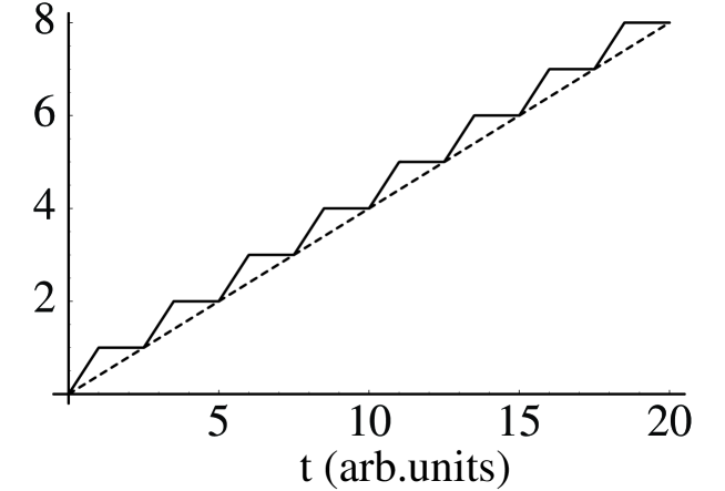
FIG. 1.: The function $F(t)$ defined in Eq. (14) (full line) is plotted as a function of time (expressed in arbitrary units) and compared with its “linear approximation”, the rescaled time $t\tau_{1}/\tau_{2}$ (dashed line). The relative error between them is given by $(\tau_{2}-\tau_{1})/t$ and is negligible at large times $t$.

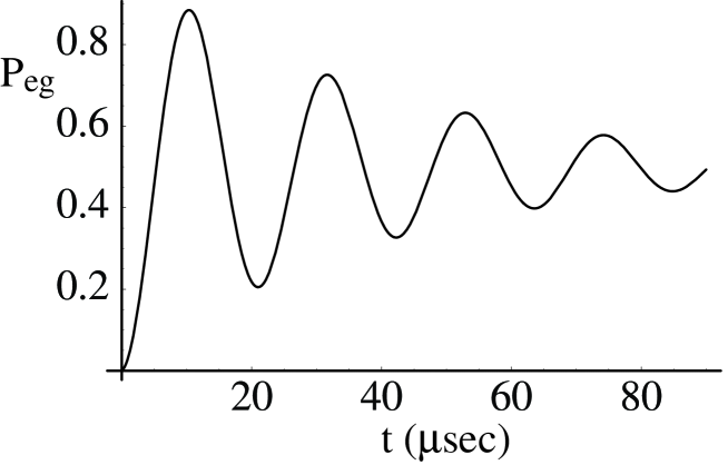
FIG. 2.: The Rabi oscillations of the transition probability $P_{eg}(t)$ as a function of time, according to the fitting function of Eq. (26).

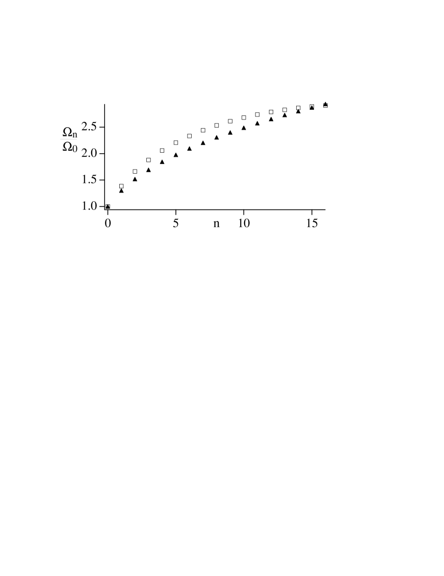
FIG. 3.: The ratio between Rabi frequencies $\Omega_{n}/\Omega_{0}$ experimentally measured in Ref. [7], and well fitted by the theoretical prediction of Eq. (45), is plotted as a function of the initial vibrational number $n$ (squares), and compared with the power-law approximation of Eq. (48), $(n+1)^{0.35}$ (triangles).

REFERENCES

- [1] W.H. Zurek, Phys. Today 44(10), 36 (1991), and references therein.
- [2] D. Giulini, E. Joos, C. Kiefer, J. Kupsch, I.O. Stamatescu, and M.D. Zeh, Decoherence and the appearance of classical world in quantum theory, (Springer, Berlin 1996).
- [3] R. Bonifacio, Nuovo Cimento 114B, 473 (1999); LANL e-print archive quant-ph/9901063.
- [4] R. Bonifacio, in Mysteries, Puzzles and Paradoxes in Quantum Mechanics, edited by R. Bonifacio, AIP, Woodbury, 1999, pag. 122.
- [5] M. Brune et al., Phys. Rev. Lett. 76, 1800 (1996).
- [6] M. Brune et al., Phys. Rev. Lett. 72, 3339 (1994).
- [7] D.M. Meekhof et al., Phys. Rev. Lett. 76, 1796 (1996).
- [8] I.S. Gradshteyn and I.M. Ryzhik, Table of Integrals and Series, Academic, Orlando, 1980, pag. 317.
- [9] G. Raithel, C. Wagner, H. Walther, L.M. Narducci, and M.O. Scully, Advances in Atomic, Molecular and Optical Physics, edited by P. Berman (Academic Press, New York, 1994), Suppl. 2, pag. 57.
- [10] M. Brune, S. Haroche, J.M. Raimond, L. Davidovich and N. Zagury, Phys. Rev. A 45, 5193 (1992).
- [11] C.M. Caves, K.S. Thorne, R.W.P. Drever, V.D. Sandberg and M. Zimmermann, Rev. Mod. Phys. 52, 341 (1980).
- [12] D.F. Walls and G.J. Milburn, Quantum Optics, Springer, Berlin, 1996.
- [13] E.T. Jaynes and F.W. Cummings, Proc. IEEE 51, 89 (1963).
- [14] J.M. Raimond, private communication.
- [15] H. Walther, and B. Varcoe, private communication.
- [16] D.J. Wineland, C. Monroe, W.M. Itano, D. Leibfried, B.E. King, D.M. Meekhof, J. Res. Natl. Inst. Stand. Technol. 103, 259 (1998).
- [17] S. Schneider and G.J. Milburn, Phys. Rev. A 57, 3748 (1998).
- [18] M. Murao, P.L. Knight, Phys. Rev. A 58, 663 (1998).
- [19] D. Wineland, private communication.
- [20] Ch. Roos, et al., LANL e-print archive quant-ph/9909038.