The Van der Waals interaction of the hydrogen molecule -
an exact local energy density functional.

Abstract

We verify that the van der Waals interaction and hence all dispersion interactions for the hydrogen molecule given by:

$$W^{\prime\prime}=-{A\over R^{6}}-{B\over R^{8}}-{C\over R^{10}}-\dots,$$ (1)

in which $R$ is the internuclear separation, are exactly soluble. The constants $A=6.4990267\dots$, $B=124.3990835\dots$ and $C=1135.2140398\dots$ (in Hartree units) first obtained approximately by Pauling and Beach (PB) [1] using a linear variational method, can be shown to be obtainable to any desired accuracy via our exact solution. In addition we shall show that a local energy density functional can be obtained, whose variational solution rederives the exact solution for this problem. This demonstrates explicitly that a static local density functional theory exists for this system. We conclude with remarks about generalising the method to other hydrogenic systems and also to helium.

]

I Introduction

Amongst the few non-trivial many-body problems in quantum mechanics, the hydrogen molecule was the first system to be thoroughly studied and continues to be researched, motivated by experiments [2],[3],[4] and by advances in modern LDA techniques of computation [5]. It is perhaps not so well known that the dispersion forces for this elementary system is amenable to an exact solution, due to certain confusion in the early literature with regard to the methods used to attack it. In this paper we shall use a method first propounded by Slater and Kirkwood (SK) [6], but whose equation (see eqn(16) below) they were unable to solve, to show that the dispersion forces for the hydrogen molecule are exactly soluble. This method later became formalised as the method of Dalgarno and Lewis [7] and is particularly suited for the problem of dispersion forces in general. However it does not seem to have been exploited in recent studies of the van der Waals interaction using density functional theories, [8], [9] . We shall demonstrate the superior convergence properties of the SK method. This was already known to the early pioneers, [1], [6], in contrast to frequency dependent methods, essentially based on a summation over dipole matrix elements with excited states or an integration over the dynamical polarizabilities. The latter was derived through the original work of Eisenchitz and London [10], and had a rather strong influence on later studies [11]. For the hydrogen system, we shall derive an exact local density functional theory, soluble for this case, and whose solution converges to the exact results. We shall show that the method is generalisable to other hydrogenic systems and also to helium for which systematic approximations can be derived. In section II, we shall discuss the background to the exact solution verifying that the PB variational method is essentially exact, though more slowly convergent than the SK method. In section III we shall present our method for solving the SK equation and show our results. In section IV we shall formulate the local density functional theory (LDFT), discuss its solution and show that it converges to the exact results of section III. In section V we shall discuss the problem of helium and conclude in section VI with discussions about further work.

II Background

The Hamiltonian for the dispersion forces of the hydrogen molecule was first derived by Margenau [12] and has appeared in subsequent editions of many textbooks, especially the famous one of Pauling and Wilson [13]. The latter contains an excellent survey of the variational treatment for the van der Waals interaction for the hydrogen molecule and also to early results for the helium system, which to this author’s knowledge has not yet been updated. As is now well known, the form of the Hamiltonian, derives essentially from a large distance expansion of the electron-electron interaction for the hydrogen molecule. This is given by [12]:

$$H^{\prime} = (1/R^{3})(x_{1}x_{2}+y_{1}y_{2}-2z_{1}z_{2})+$$ (2)

$$+ {3\over 2}(1/R^{4})[r_{1}^{2}z_{2}-r^{2}_{2}z_{1}$$ (3)

$$+ (2x_{1}x_{2}+2y_{1}y_{2}-3z_{1}z_{2})(z_{1}-z_{2})]$$ (4)

$$+ {3\over 4}(1/R^{5})[r_{1}^{2}r_{2}^{2}-5r_{2}^{2}z_{1}^{2}-5r_{1}^{2}z_{2}^{2}$$ (5)

$$- 15z_{1}^{2}z_{2}^{2}+2(x_{1}x_{2}+y_{1}y_{2}+4z_{1}z_{2})^{2}]+\dots$$ (6)

In this expression $x_{1},y_{1},z_{1}$ are the Cartesian coordinates of electron $1$ relative to its nucleus, while $x_{2},y_{2},z_{2}$ are those of electron 2 relative to its own nucleus and the $z$ axis is directed from one nucleus to the other. The expressions contain the dipole-dipole interaction $\upsilon_{A}$(first term), the dipole-quadrupole interaction $\upsilon_{B}$(second term) and the quadrupole-quadrupole interaction $\upsilon_{C}$(third term), with the first term being the well known van der Waals attraction which is dominant for large distances $R$ - the internuclear separation. Throughout this paper we shall be using Hartree units in which $(e={\hbar}=a_{0}=1)$ and thus the absolute ground state energy $E_{0}$ which we shall require later has the unit of $1/2$ Hartree. In view of the symmetry of the various terms, it can shown [1] that the above eqn(6) is equivalent with respect to its second-order perturbation energy to the Hamiltonian:

$$H^{\prime} = -2[\alpha\ \xi_{1}\xi_{2}\cos\theta_{1}\cos\theta_{2}$$ (7)

$$+ \beta\ \xi_{1}\xi_{2}^{2}\cos\theta_{1}(3\cos^{2}\theta_{2}-1)$$ (8)

$$+ \gamma\ \xi_{1}^{2}\xi_{2}^{2}(3\cos^{2}\theta_{1}-1)(3\cos^{2}\theta_{2}-1)+\dots\ ],$$ (9)

in polar coordinates, whereby: $\xi_{1,2}=2r_{1,2},\alpha=(6)^{1\over 2}/8\ R^{-3},\beta=(30)^{1\over 2}/32\ R^{-4}\$and$\ \gamma=(70)^{1\over 2}/128\ R^{-5}$. In this section we shall briefly review some of the difficulties in an accurate determination of the constants $A,B,$ and $C$. One standard formula is the direct summation method as originally used by Eisenchitz and London [10], for the van der Waals energy :

$$\epsilon_{A}(R)=-{12\over R^{6}}\sum_{n,m}{f_{1,n}f_{1,m}\over(1-{1\over n^{2}})(1-{1\over m^{2}})(2-{1\over n^{2}}-{1\over m^{2}})},$$ (10)

where $f_{l,m}=2(E_{m}-E_{l})|z_{l,m}|^{2}$ is the oscillator strength as defined in terms of the dipole matrix elements $z_{l,m}$ between the states $(l,m)$ [11]. However, the series eqn(10) converges badly even for the discrete states and there are terms involving the matrix elements between discrete/ continuum and continuum/continuum states that are difficult to evaluate but which ultimately determine the accuracy of the result. The value for the constant $A\approx 6.47$ originally given by Eisenchitz and London [10] after much work testifies to the difficulty of this approach. Nevertheless, eqn(10) has its appeal in that it can be recast into the form of an integral over imaginary frequencies of the dynamical polarizabilities of the two atoms:

$$\epsilon_{A}(R)=-{3\over R^{6}}\int_{0}^{\infty}d\xi\ \alpha_{1}(i\xi)\alpha_{2}(i\xi),$$ (11)

from which current theories for the van der Waals interaction for more complex systems like He are based. These employ a combination of linear response and time-dependent density functional theories to obtain the polarizabilities [9]. An integral equation is ultimately involved in the solution for $\alpha_{1,2}(i\xi)$, generally involving various decoupling approximations, and thereafter the integral eqn(11) has to be performed. To the best of this author’s knowledge, none of the theories proposed so far have been tested with the exactly soluble case of the $H_{2}$ molecule [8], [9] providing added motivation for our present work.

Let us mention at the outset that the central difficulty of this problem has to do with an accurate treatment of excited states, their matrix elements with the ground state (both discrete and continuous) and the poor convergence of the series like eqn(10). These are all sticky points with the modern local density functional theories (LDFT)[14]. It has been identified by Slater and Kirkwood (SK) in their classic paper [6], that a superior method involves a direct perturbation wavefunction ansatz of the form:

$$\psi({\bf r_{1}},{\bf r_{2}})=\psi_{0}(r_{1},r_{2})[1+\phi({\bf r_{1}},{\bf r_{2}})],$$ (12)

in which $\psi_{0}$ is the ground state wavefunction of the unperturbed system. The function $\phi$ (a two particle correlation function as we shall see), satisfies the following exact differential equation, easily derived from the Schrödinger equation up to first order in $\upsilon$ which can be $\upsilon_{A},\upsilon_{B}$ or $\upsilon_{C}$ accordingly. Following the notation of SK [6], this is given by:

$${1\over 2}\nabla^{2}\phi+(\nabla\ln\psi_{0}).(\nabla\phi)-\upsilon=0.$$ (13)

SK used this equation as their basis for the treatment of the $H_{2}$ and He systems. For the moment we shall concentrate on the $H_{2}$ molecule, which by the substitution:

$$\phi={\upsilon R(\xi,\xi^{\prime})\over E_{0}}$$ (14)

leads to the differential equation (hereafter known as the SK equation) in the case of the van der Waals interaction $\upsilon_{A}$ as given by:

$${\partial^{2}R\over\partial\xi^{2}}+{\partial^{2}R\over\partial\xi^{\prime 2}} + ({4\over\xi}-1){\partial R\over\partial\xi}+({4\over\xi^{\prime}}-1){\partial R\over\partial\xi^{\prime}}$$ (15)

$$- R({1\over\xi}+{1\over\xi^{\prime}})-{1\over 4}=0.$$ (16)

Note that $R(\xi,\xi^{\prime})$ is strictly non-local, but it can in principle be derived from a local density, as we shall see. Unfortunately SK were unable to solve this inhomogeneous (PDE) equation and resorted to various approximations, one of which is to ignore the differential terms and assume:

$$R_{0}(\xi,\xi^{\prime})=-{1\over 4}{\xi\ \xi^{\prime}\over\xi+\xi^{\prime}}.$$ (17)

They suggested that this is a good first approximation and that subsequent approximations can be obtained by substituting this into the differential function of eqn(16) and iterating. They evaluated the constant $A\approx 6.14$ using eqn(17), a result tabulated in the book of Pauling and Wilson [13], but unfortunately we have found this value to be in error. The correct approximate value should be $A\approx 6.23$. The second error in the SK paper is that their proposed iteration method does not work. In fact it is a non-convergent procedure, and attempts to employ it leads to divergent results. Earlier on in this work the author has carried out an iteration of their scheme to four orders and found the results diverging. Nevertheless SK suggested other approximation schemes like the ansatz $\lambda r^{\nu}r^{\prime\nu}$ where $\lambda$ and $\nu$ are variational parameters (see later) which they have found to give good results for both the $H_{2}$ and He systems. We shall discuss the solution of eqn(16) later in the next section. Here we shall mention the best solution for the $H_{2}$ problem to date. This was the widely cited paper of Pauling and Beach (PB) [1]. Their solution employs a general variational method in which the matrix elements for the Hamiltonian were evaluated using special orthogonal orbitals constructed for a solution to the Stark effect problem [13]. They have found these orbitals to be ideal for this problem by which all matrix elements for the interactions $\upsilon_{A,B,C}$ can be computed accordingly. Thereupon they were able to set up an infinite determinant from the secular equation which they have evaluated up to a rank of order $(26\times 26)$ to find the energies. Their results for $A=6.49903$, $B=124.399$ and $C=1135.21$ (accurate up to the last decimal) remain the most accurate to date, until our present work and is very impressive for 1935. However they cautioned that their “treatment has not led to an exact solution” owing to the uncertain nature of their variational method and the convergence properties of their wavefunctions [13]. In addition their method does not yield the expansion coefficients for the wavefunctions, needed to ensure normalisability and thereby obtain the normalisation constant $C(R)$. Furthermore their procedure cannot obtain the perturbation in the charge density which will be of interest to us here. The reader is referred to their earlier paper for information [1], many of whose details are now merely of historical interests. Neverthless, they have identified their method as identical with and is a more generalised variational form of that used by Hassé [15], who also was the first to treat the $H_{2}$ and He problems. In the next section we shall discuss the exact solution that SK had failed to obtain for eqn(16). We should note that the power of their method lies in the ability to employ the interaction function itself to project out all relevant components of the excited states for second order perturbation theory, into the two particle correlation function $R(r,r^{\prime})$. This then has a concise form satisfying an inhomogeneous PDE eqn(16). This method was later generalised to higher order perturbation theory by Dalgarno and Lewis [7] and Schwartz [16] see also Schiff [17].

III Solution of the SK equation

Having set the background to the hydrogen problem we shall next discuss the solution of the SK equation eqn(16). This is a two dimensional inhomogeneous (PDE) and we must first start by discussing the appropriate boundary conditions. This boundary value problem is unusual in that it is not of the standard Dirichlet or Neumann type as is common in electrostatics [18]. In fact there are no particular a prior boundary values apart from the requirement for the normalisability of the wavefunction, and special values such as $R(0,0)$ are determined only after the solution is obtained. Nevertheless an analogous Green’s function integral equation method which is exact is known to exist due to the work of Levi [19]. This is of no interest to us here, so that we shall merely outline the method in an appendix, but it may be useful for making connections with other integral equation methods of treating the problem, such as via linear response theory [8], [9].

The method we shall use to solve eqn(16) is gained from experience in solving the two sphere problem of classical electrostatics, [20],[21]. As we shall see the convergence of this problem by our method is superior to the electrostatic case of two spheres, which required nearly 200 terms for convergence to only two decimal places[20]. We begin by expanding the two particle correlation function in the following ansatz in terms of orthogonal polynomials:

$$R(\xi,\xi^{\prime})=\sum_{l,n}a_{l,n}H_{l}(\xi)H_{n}(\xi^{\prime}),$$ (18)

where the functions $H_{n}(x)=L^{3}_{n+1}(x)$ are defined in terms of associated Laguerre polynomials [22]. Inserting this into the SK eqn(16), it reduces to the form:

$$\sum_{l,n}a_{l,n}\Bigl{[}{(l-1)\over\xi}+{(n-1)\over\xi^{\prime}}\Bigr{]}H_{l}(\xi)H_{n}(\xi^{\prime})=-{1\over 4},$$ (19)

when use is made of the equation for Laguerre polynomials. Upon multiplying both sides of eqn(19) by:

$$\xi^{4}e^{-\xi}H_{m}(\xi)\xi^{\prime 4}e^{-\xi^{\prime}}H_{s}(\xi^{\prime})$$ (20)

and then integrating, with the use of the properties of the Laguerre polynomials, we derive the following infinite set of linear equations for the $a_{m,s}$:

$$- a_{m,s}(2sg_{m}q_{s}+2mg_{s}q_{m})+a_{m,s-1}(s+1)g_{m}q_{s-1}$$ (21)

$$+ a_{m,s+1}(s-1)g_{m}q_{s+1}+a_{m-1,s}(m+1)g_{s}q_{m-1}$$ (22)

$$+ a_{m+1,s}(m-1)g_{s}q_{m+1}=\Delta_{m,s}.$$ (23)

where:

$$g_{s} = {1\over 144}{(s-1)(s+1)!\over(s-2)!}\ ,q_{s}={(s+1)!\over(s-2)!},$$ (25)

$$\Delta_{m,s}=\delta_{m,2}\delta_{s,2}-\delta_{m,3}\delta_{s,2}-\delta_{m,2}\delta_{s,3}+\delta_{m,3}\delta_{s,3}.$$

This set of equations is readily solved symbolically using Mathematica version 3.1 on a PC. We shall present the results in the next subsection. Here we shall obtain the form of the energy expressions. Firstly, as was shown first by SK [6], for an arbitrary correlation function ${\tilde{R}}$ not necessarily satisfying eqn(16), the energy expression is given by:

$$\epsilon_{A} = {1\over(16\pi E_{0})}\int_{0}^{\infty}d{\xi}\int_{0}^{\infty}d{\xi^{\prime}}$$ (27)

$$\upsilon_{A}^{2}(\xi,\xi^{\prime}){\tilde{R}}(\xi,\xi^{\prime})\Bigl{(}{1\over 4}-{\cal L}[{\tilde{R}}(\xi,\xi^{\prime})]\Bigr{)},$$

where ${\cal L}$ is the differential operator given by the LHS of eqn(16). This form is particuarly useful when we look at density functional theories afterwards. At this point we shall merely mention that the change necessary for calculating the dipole-quadrupole energy $\epsilon_{B}$ and the quadrupole-quadrupole energy $\epsilon_{C}$ are the form of $\upsilon$ which becomes $\upsilon_{B}$ and $\upsilon_{C}$ respectively. The form of $R$ also changes which we shall call $R_{B}$ and $R_{C}$, (subscripts being only used when there is a need to avoid confusion) and so are the operators ${\cal L}_{B}$ and ${\cal L}_{C}$ . They can be obtained from the appropriate SK equations and are given by:

$${\partial^{2}R_{B}\over\partial\xi^{2}}+{\partial^{2}R_{B}\over\partial\xi^{\prime 2}} + ({4\over\xi}-1){\partial R_{B}\over\partial\xi}+({6\over\xi^{\prime}}-1){\partial R_{B}\over\partial\xi^{\prime}}$$ (28)

$$- R_{B}({1\over\xi}+{2\over\xi^{\prime}})-{1\over 4}=0,$$ (29)

and

$${\partial^{2}R_{C}\over\partial\xi^{2}}+{\partial^{2}R_{C}\over\partial\xi^{\prime 2}} + ({6\over\xi}-1){\partial R_{C}\over\partial\xi}+({6\over\xi^{\prime}}-1){\partial R_{C}\over\partial\xi^{\prime}}$$ (30)

$$- 2R_{C}({1\over\xi}+{1\over\xi^{\prime}})-{1\over 4}=0.$$ (31)

They can be solved by the same method as for $R_{A}$, the expressions for the expansion eqn(18) now being:

$$R_{B}(\xi,\xi^{\prime})=\sum_{l,n}b_{l,n}H_{l}(\xi)G_{n}(\xi^{\prime}),$$ (32)

and

$$R_{C}(\xi,\xi^{\prime})=\sum_{l,n}c_{l,n}G_{l}(\xi)G_{n}(\xi^{\prime}),$$ (33)

where $G_{n}(x)=L^{5}_{n+2}(x)$ is a higher order associated Laguerre polynomial. We note that for the exact solution ${\cal L}[R(\xi,\xi^{\prime})]=0$ from which the energy expressions are easily obtained in terms of the first few expansion coefficients. We shall collect the formulas for the various energy constants in terms of these coefficients as:

$$A = -12[a_{2,2}-a_{2,3}-a_{3,2}+a_{3,3}],$$ (34)

$$B = -270[b_{2,3}-b_{2,4}-b_{3,3}+b_{3,4}],$$ (35)

$$C = -2835[c_{3,3}-c_{3,4}-c_{4,3}+c_{4,4}].$$ (36)

Thus the energy constants can be determined to any desired accuracy using symbolic manipulation codes such as by Mathematica version 3.1 which yields the $a,b,c$ coefficients as exact fractions.

In order to check the definite convergence of the wavefunctions, a point of concern for Pauling and Beach [1], we have also computed the normalization constants for the wavefunctions in eqn(12). These are given by the integrals:

$$C_{i}(R)=\pi^{2}+{1\over E_{0}^{2}}\int d{\bf r}\int d{\bf r}^{\prime}\psi_{0}^{2}{\upsilon_{i}^{2}R_{i}^{2}},$$ (37)

where $i=A,B,C$ respectively. More appropriate expressions are given in terms of the constants $D_{i}$ where we have factored out the distance dependence $R$:

$$C_{A} = \pi^{2}(1+{D_{A}\over R^{6}}),$$ (38)

$$C_{B} = \pi^{2}(1+{D_{B}\over R^{8}}),$$ (39)

$$C_{C} = \pi^{2}(1+{D_{C}\over R^{10}}).$$ (40)

The values of $D_{i}$ can thus be obtained in a series in terms of the $a,b,c$ coefficients and computed to any desired accuracy. Of particular interest to us is a calculation of the density. This can be obtained by direct partial integration of the wavefunction in eqn(12). Since we are only interested in the density perturbation, by subtracting the unperturbed density $\rho_{0}=\pi e^{-\xi}$ for the ground state hydrogen atom, we have:

$${\delta\rho(\xi,\theta)\over\rho_{0}} = {\rho(\xi,\theta)-\rho_{0}\over\rho_{0}}$$ (41)

$$= \int_{0}^{\pi}d\theta^{\prime}\sin\theta^{\prime}\int_{0}^{\infty}d\xi^{\prime}e^{-\xi^{\prime}}\xi^{\prime 2}$$ (43)

$$\upsilon^{2}(\xi,\xi^{\prime},\theta,\theta^{\prime})R^{2}(\xi,\xi^{\prime}).$$

We shall redefine alternative functions $f_{i}(\xi)$ which we shall call “densities” and they are the main focus in this paper:

$${\delta\rho_{A}(\xi,\theta)\over\rho_{0}} = {1\over 4R^{6}}\xi^{2}\cos^{2}\theta f_{A}(\xi)$$ (44)

$${\delta\rho_{B}^{(1)}(\xi,\theta)\over\rho_{0}} = {3\over 16R^{8}}\xi^{2}\cos^{2}\theta f_{B}^{(1)}(\xi)$$ (45)

$${\delta\rho_{B}^{(2)}(\xi,\theta)\over\rho_{0}} = {5\over 64R^{8}}\xi^{4}(3\cos^{2}\theta-1)^{2}f_{B}^{(2)}(\xi)$$ (46)

$${\delta\rho_{C}(\xi,\theta)\over\rho_{0}} = {7\over 256R^{10}}\xi^{4}(3\cos^{2}\theta-1)^{2}f_{C}(\xi).$$ (47)

Note that there are two densities for B, since the dipole-quadrupole interaction is asymmetric. All these densities are readily computed from the appropriate wavefunction coefficients. For example we have:

$$f_{A}(\xi)=\sum_{n,m}\alpha_{n,m}H_{n}(\xi)H_{m}(\xi)\ {\rm etc.},$$ (48)

where:

$$\alpha_{n,m}=\sum_{l}a_{n,l}[2lq_{l}a_{m,l} - (l+1)q_{l-1}a_{m,l-1}$$ (49)

$$- (l-1)q_{l+1}a_{m,l+1}],$$ (50)

and so on. Their results will be given in the next subsection.

A Exact results

The infinite set of linear equations such as eqn(23) is truncated at each order and the solution for the coefficients $a,b,c$ are solved by the use of Mathematica on a PC accordingly. It is remarkable that the results are so fast converging unlike that for the two spheres problem in electrostatics [20]. Previously for the two spheres we have found the need to export the codes to a Silicon Graphics workstation running Mathematica, as expansions up to the order of 200 coefficients are necessary before we could obtain convergence to 2 decimal places. The present codes run readily on a PC and as the following Table I shows they converge rapidly. The superiority of convergence of our approach versus other methods [10] is obvious from the results shown in this table. Our convergence rate is even better than the calculations of PB [1].

TABLE I.: Computed constants A and $D_{A}$

order of truncation	A	$D_{A}$
1	6	6
2	6.22222222$\dots$	6.61728395$\dots$
3	6.46153846$\dots$	6.88757396$\dots$
4	6.48214285$\dots$	7.40242346$\dots$
5	6.49844398$\dots$	7.40024688$\dots$
6	6.49900257$\dots$	7.39872679$\dots$
7	6.49902535$\dots$	7.39863094$\dots$
8	6.49902659$\dots$	7.39862559$\dots$
9	6.49902669$\dots$	7.39862525$\dots$
10	6.49902670$\dots$	7.39862522$\dots$

TABLE II.: Computed constants B and $D_{B}$

order of truncation	B	$D_{B}$
1	115.71428571$\dots$	24.79591836$\dots$
2	118.96875	26.74423828$\dots$
3	124.26672692$\dots$	30.14754412$\dots$
4	124.39502505$\dots$	30.12987113$\dots$
5	124.39891831$\dots$	30.12699933$\dots$
6	124.39907397$\dots$	30.12683881$\dots$
7	124.39908277$\dots$	30.12682990$\dots$
8	124.39908349$\dots$	30.12682930$\dots$
9	124.39908357$\dots$	30.12682924$\dots$
10	124.39908358$\dots$	30.12682924$\dots$

Here we see that at truncation order 10, where there are about 100 coefficients, the smallest being $a_{10,10}$, we have achieved convergence to at least seven decimal places. Our results are in exact agreement with Pauling and Beach [1], indicating that they have indeed found the exact energy variationally. In particular the normalisation constants converge to the same accuracy indicating that the wavefunctions are normalisable and thus well behaved. In the following Fig.1 we shall show the computed density function $f_{A}(\xi)$.

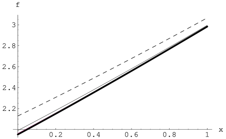
FIG. 1.: Computed density function $f_{A}(\xi)$ for successive truncations from order 5 (dashes). Note the convergence in the successive plots towards the solid curve.

TABLE III.: Computed constants C and $D_{C}$

order of truncation	C	$D_{C}$
1	1063.125	199.3359375
2	1132.610294117$\dots$	238.583207179$\dots$
3	1135.107421875	238.686733245$\dots$
4	1135.208820466$\dots$	238.645331783$\dots$
5	1135.213725627$\dots$	238.641796376$\dots$
6	1135.214015982$\dots$	238.641543683$\dots$
7	1135.214037581$\dots$	238.641524775$\dots$
8	1135.214039617$\dots$	238.641523160$\dots$
9	1135.214039858$\dots$	238.641522996$\dots$
10	1135.214039892$\dots$	238.641522976$\dots$

It is to be noted that the large distance behaviour in the density dictates the subsequent accuracy in the energy calculation. We show the density at various orders in Fig.2.

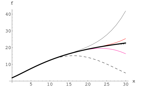
FIG. 2.: Computed density function $f_{A}(\xi)$ at larger distances for successive truncations. Order 5 is the bottom curve (dashes) while order six is the top curve (line). The curves have alternative curvatures for odd and even orders of truncation. Note the convergence to the middle plots at higher orders and the difference with the scale of Fig.1.

In a similar way we have computed the B and C energy constants in eqn(1), as well as their respective normalisation constants $D_{B}$ and $D_{C}$ respectively. These are shown in Tables I and II. Note that the numbers are tabulated as decimals for convenience, but they are exact fractions as given by Mathematica. As such some of the numbers terminate as decimals, whereas the others have a finite period, most of which are much longer than the 8 or 9 decimals shown. For completeness of the results we have plotted all the various density functions calculated from the exact wavefunction coefficients.

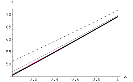
FIG. 3.: Computed density function $f_{B}^{(1)}(\xi)$ for successive truncations from order 5 (dashes), as in Fig.1.

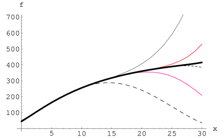
FIG. 4.: Computed density function $f_{B}^{(1)}(\xi)$ at larger distances, for successive truncations from order 5 (bottom curve), as in Fig.2.

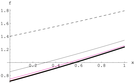
FIG. 5.: Computed density function $f_{B}^{(2)}(\xi)$ for successive truncations from order 5 (dashes), as in Fig.3.

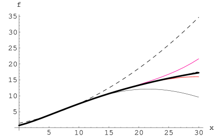
FIG. 6.: Computed density function $f_{B}^{(2)}(\xi)$ at larger distances for successive truncations from order 5 (bottom curve), as in Fig.4

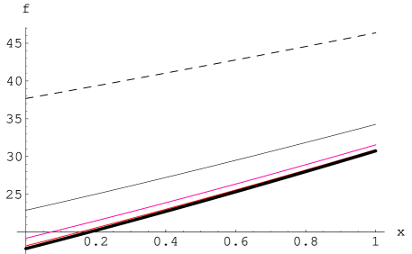
FIG. 7.: Computed density function $f_{C}(\xi)$ for successive truncations from order 5 (dashes), as in Fig.5 .

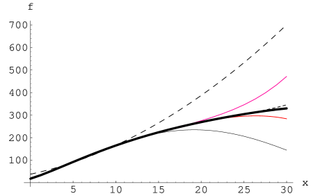
FIG. 8.: Computed density function $f_{C}(\xi)$ at larger distances for successive truncations from order 5 (bottom curve), as in Fig.6

Note that for shorter distances in figures 1,3,5 and 7, the convergence proceeds monotonically from the top curve to the bottom. These plots are nearly straight, but for larger distances they have alternative curvatures for odd and even truncation orders. These observations furnish interesting approximation methods, which will not be investigated here. In the next section, we shall use the results obtained so far to derive an exact local density functional theory for this system.

IV An exact energy local density functional

Current thinking in density functional theory (DFT) approaches the problem of dispersion forces from eqn(11), as mentioned earlier, via time-dependent generalisations of DFT. It is interesting to note that the method of Kohn et al [9] has yielded results in agreement with the best theoretical value for He up to two decimal places, in spite of a 7% error in the completeness sum rule in their calculations. However it is difficult from these theories to develop systematic improvement methods and would require considerable expertise in time-dependent density functional methods. The question arises a long ago in a paper pointed out by Lieb [23], that the universal Hohenberg-Kohn (HK) functional $I[\rho]$ [24] has “hidden complexities” with respect to the van der Waals interaction. The dynamical dipole fluctuation properties leading to the latter “is somehow built into $I[\rho]$, but an explicit form of $I[\rho]$ that will produce this effect has yet to be displayed.” This is in spite of a very general proof for the universal character of van der Waals forces for Coulomb systems [25]. We shall answer this question some way for the $H_{2}$ molecule. It is noteworthy that perhaps as a result of these remarks, the search for an accurate static local density functional theory for dispersion forces has more or less been abandoned. In this section we shall demonstrate that for the $H_{2}$ molecule system at hand we can formulate an exact static DFT. We start from the observation that the two particle correlation $R(r,r^{\prime})$ is a functional of the density $f_{A}$. In eqn(48) if the quantities $\alpha_{n,m}$ are fixed, thereby fixing the density, then eqn(50) in principle can be inverted to obtain the coefficients $a_{n,m}$ thereby determining $R(r,r^{\prime})$. Therefore upon substituting this $R[\alpha_{n,m}]$ into the energy functional eqn(27), then a variation of $\epsilon_{A}$ with respect to $\alpha_{n,m}$ would yield the exact ground state energy. This corresponds to the constraint search algorithm of Levy [26], but note that this is not the HK functional as it is specific to this problem. Formally we can write this as:

$$\epsilon_{A} = {1\over(16\pi E_{0})}\int_{0}^{\infty}d{\bf\xi}\int_{0}^{\infty}d{\bf\xi^{\prime}}$$ (52)

$$\upsilon_{A}^{2}(\xi,\xi^{\prime}){\tilde{R}}[f_{A}(\xi)]\Bigl{(}{1\over 4}-{\cal L}[{\tilde{R}}[f_{A}(\xi)]]\Bigr{)}.$$

Then the ground state energy and density can be obtained from:

$${\delta\epsilon_{A}[f_{A}(\xi)]\over\delta f_{A}(\xi)}=0.$$ (53)

However eqn(50) is not the most convenient to use. Its inversion corresponds to a non-linear programming problem with many solutions. This complexity came from our choice of orbitals which for the exact solution fixes: ${\cal L}[R[f_{A}(\xi)]]=0$. An alternative choice of orbitals can be made which then fixes ${\tilde{R}}[f_{A}(\xi)]$ but now ${\cal L}[{\tilde{R}}[f_{A}(\xi)]]\not=0$. Nevertheless eqn(53) will still yield the exact ground state energy via eqn(52) which is the essence of our DFT.

A convenient choice of orbitals is determined from the density expression:

$$f_{A}(\xi)=\int_{0}^{\infty}d\xi^{\prime}e^{-\xi^{\prime}}\xi^{\prime 4}{\tilde{R}}^{2}_{A}(\xi,\xi^{\prime}).$$ (54)

It can be easily seen that the choice of orbitals $\phi_{n}(\xi)=L^{4}_{n}(\xi)$ such that:

$$f_{A}(\xi)=\sum_{n,l}{\tilde{\alpha}}_{n,l}\phi_{n}(\xi)\phi_{l}(\xi)\ {\rm etc.},$$ (55)

provide a much simpler form for the density whereupon:

$${\tilde{R}}_{A}(\xi,\xi^{\prime})=\sum_{n,m}{\tilde{a}}_{n,m}\phi_{n}(\xi)\phi_{m}(\xi^{\prime}),$$ (56)

where:

$${\tilde{\alpha}}_{n,l}=\sum_{m}\omega_{m}{\tilde{a}}_{n,m}{\tilde{a}}_{l,m};$$ (57)

in which $\omega_{m}=m!/(m-4)!$, as appropriate for these orbitals. The variation of the density $f_{A}$ can now be effected by directly varying the coefficients ${\tilde{a}}_{n,m}$. The latter can be easily computed from eqn(53), which can be carried out symbolically as well. The integrals required throughout the calculation can also be computed in closed form, facilitated by the symbolic integration capabilities of Mathematica. Our results are tabulated in Table IV. The results are in exact agreement with Table I, since as we have noted earlier the output are exact numeric fractions that can be compared order by order with the results of the subsection III A. The integrals involved are somewhat more lengthy here so that we have not extended the calculations beyond the 6th order. In the following figures, we have plotted the density functions which are again in exact agreement with the previous figures 1 and 2.

FIG. 9.: Computed density function $f_{A}(\xi)$ truncated at order six, the dotted curve is our exact DFT result and the solid curve is the exact result of the previous section. Both curves are identical.

TABLE IV.: Computed constant A using our DFT eqn(53

order of truncation	A
1	6
3	6.46153846$\dots$
4	6.48214285$\dots$
5	6.49844398$\dots$
6	6.49900257$\dots$

FIG. 10.: Computed density function $f_{A}(\xi)$ for truncations at order 6 for larger distances. The dash curve is our exact DFT result and the solid curve is the exact result of the previous section, both curves are seen to be identical.

We can show in the same way using the exact DFT for the other energy constants B and C that they yield identical results as subsection III A. The convenient orbitals for these other density expansions are easily seen to be: $\phi_{n}(\xi)\chi_{m}(\xi)$ for $f_{B}^{(1)}(\xi)$ and $\chi_{n}(\xi)\chi_{m}(\xi)$ for $f_{B}^{(2)}(\xi)$ and $f_{C}^{(2)}(\xi)$ accordingly, where $\chi_{n}(\xi)=L^{6}_{n}(\xi)$. We found these results to be very instructive from the viewpoint of DFT. In particular approximate densities can be developed. For example the form:

$$f_{A}(\xi)={\rm Const}\quad\xi^{2\nu},$$ (58)

with Const $=\lambda^{2}(4+2\nu)!$ follows from the SK ansatz for $R(r,r^{\prime})=\lambda r^{\nu}r^{\prime\nu}$. The variational results using this approximation (which have to be computed numerically) give two significant figures accuracy except for the case of $\epsilon_{B}$, see Table V.

TABLE V.: Computed constants A,B and C using eqn(58)

A	B	C
6.48965	116.795	1134.71

The following figures compare the approximate with the exact densities. We shall not discuss these approximations here as detail investigations will require further work. In the next section we shall discuss if our results could be extended as approximate methods for more complex systems for which no exact solutions are known.

FIG. 11.: Approximate density function $f_{A}(\xi)$ (dashed) calculated from eqn(58) compared with the exact one.

FIG. 12.: Approximate density function $f_{B}^{2}(\xi)$ (dashed) calculated from eqn(58) compared with the exact one. Note that this poor density also yields a poor energy constant.

FIG. 13.: Approximate density function $f_{C}(\xi)$ (dashed) calculated from eqn(58) compared with the exact one. Note that this good density also yields a good energy constant.

V Hydrogenic systems and helium

For hydrogenic atoms for which we can replace the core charge from $Z=1$ by $Z^{\prime}$ say, the modifications of our method is quite straightforward. A first principles calculation however is a different matter. We shall only discuss the van der Waals energy $\epsilon_{A}$ from hereon. This can be seen by considering the helium problem. The interaction energy contains a sum of interactions taken from all possible pairs of electrons between the two atoms:

$$\upsilon=\sum_{j=1}^{N}\sum_{k=1}^{N}\upsilon_{j,k},$$ (59)

where $N$ is the number of electrons on each atom and:

$$\upsilon_{j,k}=(1/R^{3})(x_{j}x_{k}+y_{j}y_{k}-2z_{j}z_{k}).$$ (60)

The two particle correlation function eqn(14) now breaks up into a sum of pairs:

$$\phi({\bf r}_{j},{\bf r}_{k})={1\over E_{0}}\sum_{j=1}^{N}\sum_{k=1}^{N}\upsilon_{j,k}R(r_{j},r_{k}),$$ (61)

and the SK eqn(16) now becomes a set of $N^{2}$ equations:

$${\partial^{2}R\over\partial\xi_{j}^{2}} + {\partial^{2}R\over\partial\xi_{k}}+({4\over\xi_{j}}+2{\partial\ln\psi_{0}\over\partial\xi_{j}}){\partial R\over\partial\xi_{j}}+({4\over\xi_{k}}+2{\partial\ln\psi_{0}\over\partial\xi_{k}}){\partial R\over\partial\xi_{k}}$$ (62)

$$+ 2R({1\over\xi_{j}}{\partial\ln\psi_{0}\over\partial\xi_{j}}+{1\over\xi_{k}}{\partial\ln\psi_{0}\over\partial\xi_{k}})-{1\over 4}=0.$$ (63)

These equations are now coupled, since in general $\psi_{0}$ is a many-body wavefunction. Hence the problem is in general insoluble. Nevertheless, the situation in which $\psi_{0}$ is given in an LDA approximation as a product of Kohn-Sham (KS) orbitals [27] is greatly simplified and should form the basis of an LDA approach as we shall see . We have learnt from the hydrogen problem that the correlation function $R(r_{j},r_{k})$ and the density $f(r_{j})$ are closely connected with these orbitals. For hydrogenic atoms in which the core can be considered as a closed shell, then the following approximation:

$${\partial\ln\psi_{0}\over\partial\xi_{j,k}}\approx-Z^{\prime}/2,$$ (64)

where $Z^{\prime}<1$ can be made without a significant lost of accuracy. In this case eqn(63) reduces to a single equation and is amenable to analytical treatment as for hydrogen. However from the form of the energy, which is additive in terms:

$$\epsilon=\sum_{j=1}^{N}\sum_{k=1}^{N}\epsilon_{j,k},$$ (65)

where:

$$\epsilon_{j,k} = {1\over E_{0}}{\int\upsilon^{2}_{j,k}{\tilde{R}}_{j,k}(1-{\cal L}_{j,k}[{\tilde{R}}_{j,k}])\psi_{0}^{2}d\tau\over\int\psi_{0}^{2}d\tau},$$ (66)

we will be motivated to consider a DFT theory such as that presented in section IV with appropriate approximations. Note that the integral in eqn(66) is over the coordinates of all the electrons with the implicit dependence of $R_{j,k}$ on the others. As can be easily seen, the operator ${\cal L}_{j,k}$ simplifies considerably if the ground state of the atom $\psi_{g}$ is well approximated by a Hartree type, or KS type wavefunction for spherical atoms:

$$\psi_{g}=\prod_{j=1}^{N}\psi_{j}(r_{j}),$$ (67)

as in this case the eqns(63) decouple. The accuracy of the calculations will be dependent on approximations to the density $f(r_{j})$ and the wavefunction $\psi_{0}$. Further investigations along these lines will be able to provide a systematic study of van der Waals interactions as in the case of hydrogen detailed here.

VI Conclusion

This paper sets out an exact solution for the van der Waals and other dispersion forces for the hydrogen molecule using the method of Slater and Kirkwood, [6]. By considering the density distributions $f_{A,B,C}$ we have shown that in this case, an exact energy density functional exists for this problem which when minimised with respect to the density, yields the exact results. We have shown that the energy constants $A,B,C$ can be calculated to any desired accuracy, the first few decimals being in full agreement with Pauling and Beach [1]. We have also considered the extension of our method for more complex systems such as hydrogenic systems and helium for which approximations must be invoked. A systematic study of these and generalizations to include the effect of a surface [28] will be the subject of future work.

Acknowledgements: The author wish to thank the NCTS (Taiwan) for their hospitality during the final stages of this work. This paper is dedicated to the memory of J. Mahanty, who crossed path with the author during a period at the Australian National University in the late 1980’s.

Appendix

Integral equation method

The integral equation technique for solving the SK eqn(16) is due to Levi [19]. We define the operator $\cal W$ acting on any function such as $R$:

$${\cal W}[R]\equiv\Delta R+aR_{\xi}+bR_{\xi^{\prime}}+cR,$$ (68)

where the subscripts denote differentiation from hereon and $\Delta$ is the two dimensional Laplacian operator, so that the SK eqn(16) is given by:

$${\cal W}[R]=f;$$ (69)

in which:

$$a=({4\over\xi}-1) \quad b=({4\over\xi^{\prime}}-1)$$ , (70)

$$c=-({1\over\xi}+{1\over\xi^{\prime}}) \quad f=1.$$ , (71)

A uniqueness theorem for particular solutions can be proved for any value of $c\leq 0$, [19] thus guaranteeing a solution for eqn(69). With the use of an appropriate two dimensional Green’s function $G(x,y|x^{\prime},y^{\prime})$ such that:

$$\Delta G(x,y|x^{\prime},y^{\prime})=-2\pi\delta(x-x^{\prime})\delta(y-y^{\prime}),$$ (72)

then it can be easily shown that for any arbitrary function $\omega(x,y)$ the solution $R(x,y)$ is given by:

$$R(x,y) = \omega(x,y)$$ (73)

$$+ \int dx^{\prime}\int dy^{\prime}G(x,y|x^{\prime},y^{\prime})\rho(x^{\prime},y^{\prime}).$$ (74)

The function $\rho(x,y)$ is given by the solution of the integral equation:

$$\rho(x,y)=\int dx^{\prime}\int dy^{\prime}K(x,y|x^{\prime},y^{\prime})\rho(x^{\prime},y^{\prime})+g(x,y),$$ (75)

where the kernel $K(x,y|x^{\prime},y^{\prime})$ is of the form:

$$K(x,y|x^{\prime},y^{\prime})={1\over 2\pi}\Bigl{(}aG_{x}+bG_{y}+cG\Bigr{)},$$ (76)

and the function $g(x,y)$ is:

$${1\over 2\pi}\Bigl{(}{\cal L}[\omega]-f\Bigr{)}.$$ (77)

That eqns(74) to (77) give a solution for eqn(69) can be easily shown by operating on $R$ in eqn(74) with the operator ${\cal W}$. With an appropriate choice of Green’s function $G(x,y|x^{\prime},y^{\prime})$ and $\omega(x,y)$, the iteration of eqn(75) is equivalent to our solution for $R(x,y)$ as obtained in section III.

REFERENCES

- [1] L. Pauling and J. Y. Beach, Phys. Rev. 47, 686 (1935).
- [2] M. Boudart et al, J. Am. Chem. Soc. 94(19), 6622 (1972).
- [3] S.L. Chin and S. Lagacé, Applied Optics 35(6), 907 (1996).
- [4] D. Kleppner, Physics Today 52(4), 11 (1999).
- [5] J. P. Perdew, K. Burke and M. Emzerhof, Phys. Rev. Lett. 77, 3865 (1996).
- [6] J. C. Slater and J. G. Kirkwood, Phys. Rev. 37, 682 (1931).
- [7] A. Dalgarno and J. T. Lewis, Proc. Roy. Soc. (London) A233, 70 (1955).
- [8] J. F. Dobson, B. P. Dinte and J. Wang, in Electronic Density functional Theory: Recent Progress and New Directions, pg 261, edited by Dobson et al., Plenum Press, New York (1998).
- [9] W. Kohn, Y. Meir and D. E. Makarov, Phys. Rev. Lett. 80(19), 4153 (1998).
- [10] R. Eisenchitz and F. London, Zeits. f. Physik, 60, 491 (1930).
- [11] J. Mahanty and B. Ninham, in Dispersion Forces, Academic Press, New York (1976).
- [12] H. Margenau, Phys. Rev. 38, 747 (1931).
- [13] L. Pauling and E. B. Wilson, in Introduction to Quantum Mechanics With Applications to Chemistry, McGraw-Hill, Tokyo (1935).
- [14] See for example Density Functional Theory II, Vol 181 of Topics in Current Chemistry edited by R. F. Nalewajski, Springer, Berlin (1996).
- [15] H. R. Hassé, Proc. Camb. Phil. Soc. 27, 66 (1931).
- [16] C. Schwartz, Ann. Phys. (NY) 6, 156 (1959).
- [17] L. Schiff, Quantum Mechanics, McGraw-Hill, Tokyo (1968).
- [18] J. D. Jackson, Classical Electrodynamics, Wiley, New York (1975).
- [19] R. Courant and D. Hilbert, Methods of Mathematical Physics Vol II, Interscience, New York (1953).
- [20] T.C. Choy, Aris Alexopoulos and M.F. Thorpe, Proc. Roy. Soc. (London) A454, 1973 (1998).
- [21] T.C. Choy, Aris Alexopoulos and M.F. Thorpe, Proc. Roy. Soc. (London) A454, 1993 (1998).
- [22] Readers should note that there are two slightly different definitions of Laguerre polynomials . We use the one for physicists [13],[17], which differs from the one for mathematicians , such as defined in Mathematica v 3.1 or in most table of integrals. The difference is given by: which is a nasty source of errors as this author has found.
- [23] E. H. Lieb, Intl. J. Quantum Chem. XXIV, 243 (1983).
- [24] P. Hohenberg and W. Kohn, Phys. Bev. B136, 864 (1964).
- [25] E. H. Lieb and W. Thirring, Phys. Rev. A34(1), 40 (1986).
- [26] M. Levy, Proc. Natl. Acad. Sci., USA, 76(12), 6062 (1979).
- [27] W. Kohn and L. J. Sham, Phys. Rev. , A140,1133 (1965).
- [28] T.C. Choy and B. C. den Hertog, J. Phys. Condens. Matter , 7,19 (1995).