Evaluation of heating effects on atoms trapped in an optical trap

Abstract

We solve a stochastic master equation based on the theory of Savard et al. [T.A. Savard, K.M. O’Hara and J.E. Thomas, Phys. Rev. A56, R1095 (1997)] for heating arising from fluctuations in the trapping laser intensity. We compare with recent experiments of Ye et. al. [J. Ye, D.W. Vernooy and H.J. Kimble, Trapping of single atoms in cavity QED, quant-ph/9908007, Phys. Rev. Lett. (1999), in press], and find good agreement with the experimental measurements of the distribution of trap occupancy times. The major cause of trap loss arises from the broadening of the energy distribution of the trapped atom, rather than the mean heating rate, which is a very much smaller effect.

In a far-off resonance red-detuned trap, the effective potential of the trapped atom can be written

$$V(x)=-{1\over 4}\alpha|{\cal E}(x)|^{2}$$ (1)

where $\alpha$ is the atomic polarizability, and ${\cal E}(x)$ is the slowly varying field amplitude [1, 2]. Following [1], the heating can be modeled using a Hamiltonian for a trapped atom of mass $M$ of the form

$$H={p^{2}\over 2M}+{1\over 2}M\omega_{\rm tr}^{2}[1+\epsilon(t)]x^{2},$$ (2)

which leads to transition probabilities between trap levels of the form

$$R_{n\pm 2\leftarrow n}={\pi\omega_{\rm tr}^{2}\over 16}S_{\epsilon}(2\omega_{\rm tr})(n+1\pm 1)(n\pm 1).$$ (3)

In these equations, $\epsilon(t)$ is a fluctuating quantity, whose spectrum is

$$S_{\epsilon}(\omega)\equiv{2\over\pi}\int_{0}^{\infty}d\tau\,\cos(\omega\tau)\langle\epsilon(t)\epsilon(t+\tau)\rangle.$$ (4)

From these transition probabilities, in follows that the time dependent probability $P(n)$ that a single atom is in the $n$th level of the trap under the influence of the fluctuation field satisfies the stochastic master equation

$$\dot{P}(n) = {\Gamma_{\epsilon}\over 8}\bigg{\{}(n+2)(n+1)P(n+2)+n(n-1)P(n-2)$$ (6)

$$-[n(n-1)+(n+2)(n+1)]P(n)\bigg{\}}.$$

with the rate constant

$$\Gamma_{\epsilon}\equiv\pi^{2}\nu_{\rm tr}^{2}S_{\epsilon}(2\nu_{\rm tr}).$$ (7)

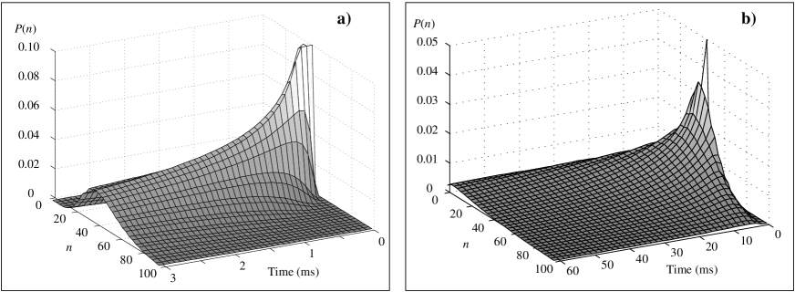
FIG. 1.: Evolution of the probability distribution $P(n)$: a) Plotted on a short timescale, it can be seen that the heating spreads the initial sharp distribution in less than 2ms to cover nearly the full height of the trap; b) Over the full timescale of the experiment losses continue at a steady rate. The heating rate used is $1/\Gamma_{\epsilon}=1/\Gamma_{\epsilon}^{\rm axial}=23{\rm ms}$.

As shown in [1], this constant is equal to the mean heating rate, defined as the rate of increase of the level number (proportional to the energy) of the atom in the trap, i.e.,

$${d\langle n\rangle\over dt}=\Gamma_{\epsilon}\langle n\rangle.$$ (8)

It should be noted, however, that this heating rate arises as the difference $R_{n+2\leftarrow n}-R_{n-2\leftarrow n}$, in which the quadratic terms cancel. If $n$ is significantly different from zero—perhaps about 50 in [3]—the positive and negative contributions to the heating rate will both be very much larger than the heating rate itself. Thus the result of the heating process will be principally to spread the distribution over the energy levels, superimposed on a much slower increase in the average energy according to (8). In fact, the principal time constant for the growth of $\sigma$, the standard deviation of $n$, is $3\Gamma_{\epsilon}/2$.

The principal effect of the heating in the experiment of [3] is to expel the atom from the trap, and in general this will occur not as a result of the increase of the average energy, but rather as a result of the rapid spreading of the width of the distribution, so that the upper part spreads into untrapped levels.

The three-dimensional trap used in [3] was sinusoidal longitudinally, and had a Gaussian form radially. Approximating both of these by harmonic fluctuation traps, it was found by measuring the fluctuation spectrum that

$$1/\Gamma_{\epsilon}^{\rm radial} \approx 830{\rm ms}$$ (9)

$$1/\Gamma_{\epsilon}^{\rm axial} \approx 23{\rm ms}.$$ (10)

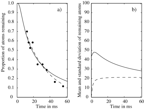
FIG. 2.: a) Solid line: Computed probability for the atom to remain trapped when the initial mean excitation is the 45th level—heating rate as in Fig.1; Points: Experimental data from [3]; Dashed line: exponential fit to data. b) Solid line: Mean excitation of an atom remaining in the trap; Dashed line: Standard deviation of the excitation.

We may safely neglect the much slower radial heating, and treat the trap as one dimensional. The trap depth corresponds to some 100 levels, so we will model the escape process by truncating the master equation to the first 100 levels—once the atom leaves this range it ia assumed not to return. The equation is easy to solve. As an initial condition, we assume the atom is evenly distributed between the levels $N_{0}$ and $N_{0}+1$ , with $0\leq N_{0}<100$. The results of a simulation with $N_{0}=45$ are shown in Fig.1. The very rapid spreading of the probability distribution from its initally sharply peaked form is very clear. In fact very little difference results if a less sharply peaked initial distribution is used, even for a width of about 20 levels. The probability that the atom remains in the trap is plotted in Fig. 2a, and this fits the experimental data remarkably well. However, the result is not exponential, though there is a strong similarity. Points to note are

• From Fig. 1 and Fig. 2 it can be seen that a population around $n=0$ is rapidly produced, and this decays very slowly, because the relevant transition probabilities are very small. That this is not observed in practice may be the result of the existence of other heating mechanisms.

• The heating rate $\Gamma_{\epsilon}$ does correctly give the timescale of the heating process, even though the details of the heating process are not themselves well summarized by (8).

To counter this heating effect one can conceive of introducing some kind of laser cooling. One would expect that provided the cooling time is sufficiently smaller than the heating time, one should be able to ensure that the atom remains trapped. We can model cooling by use of a standard master equation coupling to a heat bath, such as in [4], which would give an additional contribution to the stochastic master equation (6)

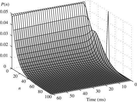
FIG. 3.: Evolution of the probability distribution $P(n)$ with both heating and cooling. The heating rate used is $1/\Gamma_{\epsilon}=1/\Gamma_{\epsilon}^{\rm axial}=23{\rm ms}$, and the cooling rate is $\Gamma_{\rm cool}=2{\rm ms}$

$$\left.\dot{P}(n)\right|_{\rm cool} = \Gamma_{\rm cool}\Big{\{}(\bar{N}+1)[(n+1)P(n+1)-nP(n)]$$ (12)

$$+\bar{N}[nP(n-1)-(n+1)P(n)]\Big{\}}$$

In this equation the effective temperature of the heat bath is determined by the mean excitation, $\bar{N}$, which the bath acting by itself would produce in the trap, and $\Gamma_{\rm cool}$ is the inverse cooling time. Adding this cooling term to the heating from (6), we see in Fig.3 that the cooling very rapidly counteracts the heating. However, in Fig.4 we note that even with quite strong cooling, corresponding to $1/\Gamma_{\rm cool}\approx 2{\rm ms}$, the probability of remaining in the trap after 60ms is only 90%. By solving the equations using only the cooling part (12), it can be verified that most of the loss is in fact a residual effect of the heating.

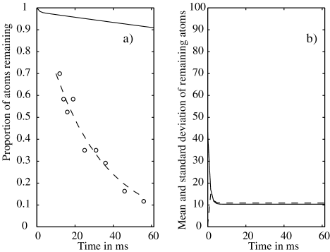
FIG. 4.: a) Solid line: Computed probability with both heating and cooling. for the atom to remain trapped when the initial mean excitation is the 45th level—heating and cooling rates as in Fig.3.; Points: Experimental data from [3]; Dashed line: exponential fit to data. b) Solid line: Mean excitation of an atom remaining in the trap; Dashed line: Standard deviation of the excitation when both heating and cooling are present.

However we cannot ensure better trapping simply by increasing the cooling rate, since the cooling has the effect of cooling to a certain residual temperature, and at any non-zero temperature there will always be some probability of escaping from the trap, even in the absence of the heating effect. Increasing $1/\Gamma_{\rm cool}$ at fixed $\bar{N}$ (i.e., fixed temperature) is equivalent to reducing the timescale of the dynamic processes involved. Once the cooling is fast enough to overwhelm the heating, any further increase will simply speed up the residual process of trap loss. The only way to get more effective confinement is then to reduce the temperature to which one cools. With this model of cooling and with $\bar{N}=10$, one finds that the best confinement is obtained with $1/\Gamma_{\rm cool}\approx 1{\rm ms}$, although this is only marginally better than the case of $1/\Gamma_{\rm cool}\approx 2{\rm ms}$ shown in the figures.

In conclusion one should bear in mind that the model of a truncated harmonic trap is very crude. In the case considered here the noise is of the order of 20% of the signal, which also means that the validity of the perturnbation theoretic calculation used by [1] to derive the transition probabilities (3) will also be marginal at best. However the only realistic alternatives to this very simple picture would involve extensive numerical work, such as direct simulation of a stochastic differential equation, or detailed computations of spectra and matrix elements for the appropriate potential.

Acknowledgements: This work was funded by the Royal Society of New Zealand under the Marsden Fund cotract PVT902; by the NSF, by DARPA via the Quantum Information and Computing Program administered by ARO, and by the ONR. HCN and JY are supported by a Millikan Prize Postdoctoral Fellowship.