Scattering of short laser pulses from trapped fermions

Abstract

We investigate the scattering of intense short laser pulses off trapped cold fermionic atoms. We discuss the sensitivity of the scattered light to the quantum statistics of the atoms. The temperature dependence of the scattered light spectrum is calculated. Comparisons are made with a system of classical atoms who obey Maxwell-Boltzmann statistics. We find the total scattering increases as the fermions become cooler but eventually tails off at very low temperatures (far below the Fermi temperature). At these low temperatures the fermionic degeneracy plays an important role in the scattering as it inhibits spontaneous emission into occupied energy levels below the Fermi surface. We demonstrate temperature dependent qualitative changes in the differential and total spectrum can be utilized to probe quantum degeneracy of trapped Fermi gas when the total number of atoms are sufficiently large $(\geq 10^{6})$. At smaller number of atoms, incoherent scattering dominates and it displays weak temperature dependence.

03.75.Fi,42.50.Fx,32.80.-t

I Introduction

Rapid advances of trapping and cooling of alkali atoms [1] have led to the recent dramatic achievement of Bose-Einstein condensation (BEC) [2, 3, 4, 5]. Focusing these highly successful trapping and cooling methods onto fermions instead of bosons offers additional rich opportunities for studying degenerate fermionic atomic gases. The description of these magnetically trapped Fermi gases presents additional simplification as the Pauli exclusion principle forbids the unsuppressed low energy s-wave collisions among atoms in the same hyperfine state. Thus these dilute trapped atoms behave very close to the ideal Fermi gas so ubiquitous in physics textbooks for decades. Recent highlights from several leading experimental groups have indicated that we are at the edge of being able to explore quantum degenerate Fermi gas [6, 7] inside laboratories.

Once such a degenerate gas is achieved, how do we perform diagnostic measurements on its properties ? A standard method in atomic physics is to probe the gas with light scattering. This is the problem to be addressed in our paper. These spectroscopic light scattering methods have already been suggested for BEC in both the weak and strong field scattering regimes [8, 9]. These early theoretical investigations had limited impact on BEC experimental observations so far, partly because the resonant photon-atom interaction becomes a complicated many body problem when a condensate is involved. The recent dramatic demonstration of low group velocity of light propagation inside a condensate [10], the Bragg scattering experiment [11], and the surprising observation of super-radiant collective spontaneous emission from MIT [12] all call for more detailed applications of quantum field theory of photons interacting with atoms. In the last several years, light scattering off Fermi degenerate atoms have already been discussed by several groups; some of these investigations focused on the case of a distribution of ideal atoms obeying Fermi-Dirac statistics [13]; while others considered more exotic state for a Cooper paired fermionic condensate [14]. One notable feature for a Fermi degenerate gas is that the Pauli exclusion principle blocks (inhibits) scattering events for atoms into already occupied states [15]. This paper aims at detailed quantitative information of light scattering from trapped Fermi gases within parameter regimes of current/future experiments, specifically results explicitly demonstrating temperature and quantum statistical effects are sought.

In a previous paper involving two of us (LY and ML) an optical method for detection of the properties of BEC was proposed [16]. This detection involves the limiting case of scattering short but intense laser pulses from a system of cooled bosonic atoms in a trap. In particular, the case of laser pulses with areas of 2$\pi K$ was investigated. (The pulse area to be defined later is proportional to the integral of the slowly varying envelope of the electric field multiplied by the atomic dipole moment). It was shown that such pulses mainly cause cyclic Rabi oscillations for atoms in their excited and ground states. Thus to zero-th order involves no photon scattering (except the stimulated interaction with the driving field). However, atoms can spontaneously emit photons while in their excited states, therefore, the previous zero-th order picture involving coherent evolution of all atoms can be interrupted by spontaneous emissions of individual atoms. Thus scattered light from these emissions can be collected and their properties reflect to a certain degree the properties of the trapped atoms. It was shown that for the case of BEC, above the critical temperature, $T_{c}$, the coherent scattering is very weak and is predominately in the forward direction due to phase matching effects. However, below the critical temperature the number of scattered photons increases dramatically and the coherent scattering occurs within a solid angle determined by the size of the condensate. For sufficiently short $2\pi K$-pulses the system is preserved even below $T_{c}$ so that this method can be potentially used as a non-destructive probe of BEC.

This paper presents a continuation of our investigations to the case of a system of trapped fermionic atoms. The ideal gas of a Fermi-Dirac distribution is considered in this paper. The static properties of harmonic trapped ideal fermionic atoms as considered by several groups previously will be used as inputs [17]. The more subtle case involving a weak attractive interactions between atoms could potentially develop into a BCS type Cooper paired condensate [18], and whose pulsed light scattering properties [14] will be explored in a future publication. In the present study involving ideal non-interacting fermionic atoms, we do not expect to see a dramatic change in the spectrum as one cools the gas since no phase transition occurs in the trapped gases even at zero temperature. However, with a finite number of atoms (say $1$ million) and cooled far below the Fermi temperature [6] one does expect that the quantum statistics should play a role in the spectrum. Indeed, we demonstrate that when number of atoms are sufficiently large such that coherent scattering dominates, spectrum of scattered light exhibits qualitative changes in its temperature dependence, a signature potentially useful to probe quantum degeneracy of the system.

The organization of the paper is as follows; first we review the formulation as was presented previously [8] for trapped bosons. In the second quantized form, the only difference lies at the commutation relations between atomic operators. We then calculate the spectra of scattered light taking into account the fermionic nature of the atomic operators. In Sect. II, we present the formulation of our model system. The near resonant laser pulse is assumed to be intense so that its interaction with trapped atoms is taken to be the zeroth order coherent process for which exact analytical solutions for the dynamics of atomic operators are given. In Sect. III, the interaction of weak scattered light with trapped atoms is treated quantum mechanically with perturbation method. The zeroth order solution of atomic operators from Sect. II is used to evaluate the dynamics of scattered photons. In Section IV, our new results for the total and differential spectrums of scattered photons are then displayed numerically. A discussion section follows where both the angular and spectral distributions are presented. We also find the total number of atoms scattered for typical experimental parameter sets. Finally we conclude with a summary of the essential physics learned from this investigation. In the appendix we show how we can re-write the expression for the spectrum of the coherently scattered light in a form that is suitable for numerical calculation.

As will become obvious by the introduction of many newly derived analytic formulae, the trapped fermion case is numerically far more difficult to calculate than the previous bosonic one. At low temperatures the fermionic system consists of many stacked energy levels [17] whereas the bosonic system nicely condenses to a few of the lowest energy levels. Also the numerical methods for infinite series summations used previously for bosons are only applicable for the high temperature regime of a Fermi gas. New methods are therefore developed to cope with the additional difficulties of the fermionic system.

The first few sections of this paper follows closely to the BEC situation. Initially the treatment is formally the same for both bosons and fermions, the only difference being the commutation relations. However, these differences become significant later especially with the calculation of the spectrum.

II The model

We consider a system consisting of $N$ fermionic atoms confined in a trap interacting with light. Let us write down its Hamiltonian in the Fock representation and in the second quantized form [8] :

$${\cal H} = \sum_{\vec{n}}\omega_{\vec{n}}^{g}g_{\vec{n}}^{{\dagger}}g_{\vec{n}}+\sum_{\vec{m}}(\omega_{\vec{m}}^{e}+\omega_{0}){\vec{e}}_{\vec{m}}^{\;{\dagger}}{\vec{e}}_{\vec{m}}$$ (1)

$$+ \sum_{\vec{n},\vec{m}}\sum_{\mu}\int d{\vec{k}}\varrho(k)\big{[}\eta_{\vec{n}\vec{m}}({\vec{k}})g_{\vec{n}}^{{\dagger}}a^{{\dagger}}_{{\vec{k}}\mu}{\vec{e}}_{\vec{m}}\!\cdot{\vec{\epsilon}}_{{\vec{k}}\mu}+{\rm h.c.}\big{]}$$ (2)

$$+ \sum_{\mu}\int d{\vec{k}}\ ck\;a^{{\dagger}}_{{\vec{k}}\mu}a_{{\vec{k}}\mu}.$$ (3)

where the Franck-Condon factors are

$$\eta_{\vec{n}\vec{m}}({\vec{k}})=\langle{g},{\vec{n}}|e^{-i{\vec{k}}\cdot{\vec{R}}}|{e},{\vec{m}}\rangle$$ (4)

with $\vec{R}$ denoting the position operator of the atom (its nucleus). We have used atomic units (unless otherwise stated), the rotating wave and the dipole approximation. The atomic annihilation and creation operators for the $\vec{n}$-th state of the center of mass motion of the atoms in the trap are denoted by $g_{\vec{n}}$ and $g_{\vec{n}}^{{\dagger}}$ respectively. Since these operators are associated with the atoms in the ground electronic state, for the case of a spherically symmetric harmonic trap potential, $\vec{n}$ has three components $(n_{x},n_{y},n_{z})$ and energy $\omega_{\vec{n}}^{g}=\omega_{{\rm t}}(n_{x}+n_{y}+n_{z})$ where $\omega_{{\rm t}}$ is the trap frequency. The size of the trap is related to the size of the ground state of the trap potential, $a=\sqrt{1/2M\omega_{{\rm t}}}$ ($\hbar=1$). The atomic annihilation and creation operators in the excited state ${\vec{e}}_{\vec{m}}$ and ${\vec{e}}_{\vec{m}}^{\;{\dagger}}$ may experience different trap potential from that of the ground state. However, from our analysis of short pulse scattering, we find that the particular shape of the excited state potential is unimportant since atoms only spend a very short period of time in the excited state [8]. The electronic transition occurs at the frequency $\omega_{0}$. Since we are treating an $s$-state to a $p$-state transition the excited state operators are vectors ${\vec{e}}_{\vec{m}}$ and ${\vec{e}}_{\vec{m}}^{\;{\dagger}}$. Annihilation and creation operators for photons of momentum $\vec{k}$ and linear polarization ${\vec{\epsilon}}_{{\vec{k}}\mu}$ ($\mu=1,2$) are denoted by $a_{{\vec{k}}\mu}$ and $a^{{\dagger}}_{{\vec{k}}\mu}$. All atomic operators obey standard fermionic anti-commutation relations. $\varrho(k)$ is a slowly varying coupling which is dependent on $k$. Its relation to the natural linewidth is $\gamma=({8\pi^{2}k_{0}^{2}}/{3c})\big{|}\varrho(k_{0})\big{|}^{2}$, with $k_{0}=\omega_{0}/c$. For notational convenience, we will suppress the indices ${g,e}$ for the internal states. The convention being that the indices $\vec{n}$, $\vec{n}^{\prime}$ represents the center of mass states in the electronic ground potential whereas $\vec{m}$, $\vec{m}^{\prime}$ denotes the center of mass states in the excited state potentials.

Note that the strong resonant atomic dipole-dipole interaction resulting from the exchange of transverse photons is included in Eq. (3).

If the system is driven by a coherent laser pulse then we may neglect spontaneous emission effects during the pulse if the pulse is sufficiently short and intense. We can then safely substitute the electric field operator entering the interaction Hamiltonian in Eq. (3) by a $c$-number. The pulses we intend to use should have duration $\tau_{L}\leq 300$ ps or shorter, i.e. width $\gamma_{L}=1/\tau_{L}\simeq 3\times 10^{9}-10^{11}$ Hz. A first estimate shows that $\gamma_{L}\gg\gamma\simeq 2.5$ MHz, so that spontaneous emission may be neglected during the interaction time of the pulse with the atoms. The current estimate for single excitation spontaneous emission is a far better one than in the bosonic case as there is no Bose enhancement. However, the fermionic nature may come into play at very low temperatures where the effective spontaneous emission rate will be greatly reduced due to suppression by the Fermi sea of ground levels. Therefore it is a good approximation to assume that the effects of dissipative spontaneous emission and dispersive dipole-dipole interactions are small compared to the coherent driving laser during the interaction between the atoms and the laser pulse. We can then replace the product of the electric field operator ($\vec{{\cal E}}^{\,(+)}$) and the absolute value of the electronic transition dipole moment ($d$) by

$$d{\vec{{\cal E}}}^{\,(+)}\to\frac{\Omega}{2}\sum_{\mu}\int d{\vec{k}}\;{\vec{\varrho}}({\vec{k}},\mu)e^{i{\vec{k}}\cdot{\vec{R}}-ickt}.$$ (5)

The envelope of the laser pulse is defined by ${\vec{\varrho}}({\vec{k}},\mu)$. $\Omega$ is the peak Rabi frequency of the laser pulse. Using the assumption that the pulse is a plane wave packet moving in the ${\vec{k}}_{L}$ direction with a central frequency $\omega_{L}$ and a linear polarization ${\vec{\epsilon}}_{L}$, we obtain

$$d{\vec{{\cal E}}}^{(+)}\to\frac{\Omega}{2}{\vec{\epsilon}}_{L}{\cal T}\big{[}\gamma_{L}(t-{\vec{k}}_{L}\cdot{\vec{R}}/\omega_{L})\big{]}e^{i{\vec{k}}_{L}\cdot{\vec{R}}-i\omega_{L}t}.$$ (6)

The time dependent profile of the pulse, ${\cal T}(\gamma_{L}t)$ is chosen to be real and we assume a gaussian shape with a peak equal to one at $t=0$.

In order for Eq. (6) to be valid, we need ${\vec{\varrho}}({\vec{k}},\mu)$ to vary in momentum of the order of $\gamma_{L}/c\simeq 10-300$ m^-1. However, the Franck-Condon factors $\eta_{\vec{n}\vec{m}}({\vec{k}})$ vary on the scale of $\delta k$, on the order of $1/a\simeq 10^{5}\ {\rm m}^{-1}$ for low $n$. For higher $n$’s, $\delta k$ scales as $1/\sqrt{n}$, so it becomes $\sim 10^{3}$ m^-1 for the highest energy levels that are still available in the trap. Thus, we have $\delta k\gg\gamma_{L}/c$ for all $\gamma_{L}$, so we may validly replace ${\vec{k}}$ by ${\vec{k}}_{L}$ inside $\eta_{\vec{n}\vec{m}}({\vec{k}}_{L})$. Inserting this substitution into Eq. (5) and Eq. (6), Eq. (3) can be written as

$${\cal H} = \sum_{\vec{n}}\omega_{\vec{n}}^{g}g_{\vec{n}}^{{\dagger}}g_{\vec{n}}+\sum_{\vec{m}}(\omega_{\vec{m}}^{e}+\omega_{0}){\vec{e}}_{\vec{m}}^{\;{\dagger}}{\vec{e}}_{\vec{m}}$$ (7)

$$+ \frac{\Omega}{2}{\cal T}(\gamma_{L}t)\Big{[}\exp(i\omega_{L}t)\sum_{n}g_{\vec{n}}^{{\dagger}}{\vec{\epsilon}}_{L}\cdot{\vec{f}}_{n}+{\rm h.c.}\Big{]},$$ (8)

where we have re-written the operators in terms of annihilation and creation operators of wave packets of excited states which originate from the $\vec{n}$-th state of the ground state potential,

$${\vec{f}}_{\vec{n}}=\sum_{\vec{m}}\eta_{\vec{n}\vec{m}}({\vec{k}}_{L}){\vec{e}}_{\vec{m}}.$$ (9)

These annihilation operators and their conjugate creation ones also obey the standard fermionic anti-commutation relations, i.e. $\{f_{\vec{n}}^{q},f_{\vec{n}^{\prime}}^{q^{\prime}{\dagger}}\}=\delta_{\vec{n}\vec{n}^{\prime}}\delta_{qq^{\prime}}$, with $q,q^{\prime}=x,y,z$ enumerating the components of the vectors $\vec{f}_{\vec{n}}$ and $\vec{f}_{\vec{n}^{\prime}}^{{\dagger}}$. Their energies $\omega_{\vec{m}}$ also vary very slowly for their corresponding states and therefore for each of the wave packets ${\vec{f}}_{\vec{n}}$, ${\vec{f}}_{\vec{n}}^{\;{\dagger}}$, their energy can be approximated by $\omega_{\vec{n}}^{g}+\omega_{0}+k_{L}^{2}/(2M)$. This assumes that the atomic wavepackets in the excited state potential will not experience much coherent oscillation or diffusion (i.e. are in a sense frozen in shape) within the duration of the laser pulse ($\tau_{L}\ll 1/\omega_{{\rm t}}$).

The Heisenberg equations that follow from the Hamiltonian (8) now becomes linear. Thus at resonance, $\omega_{L}\approx\omega_{0}+k^{2}_{L}/(2M)$, and in the rotating frame in which $g_{\vec{n}}\to e^{-i\omega_{\vec{n}}^{g}t}g_{\vec{n}}$, ${\vec{f}}_{\vec{n}}\to e^{-i(\omega^{g}_{\vec{n}}+\omega_{L})t}f_{\vec{n}}$, they become

$${\dot{g}_{\vec{n}}}(t) = -i\frac{\Omega}{2}{\cal T}(\gamma_{L}t){\vec{\epsilon}}_{L}\cdot{\vec{f}}_{\vec{n}}(t),$$ (10)

$${\vec{\epsilon}}_{L}\cdot{\dot{{\vec{f}}_{\vec{n}}\,}}(t) = -i\frac{\Omega}{2}{\cal T}(\gamma_{L}t)g_{\vec{n}}(t).$$ (11)

They can be easily solved analytically for any pulse envelope

$$g_{\vec{n}}(t) = g_{\vec{n}}(-\infty)\cos\big{[}A(t)\big{]}$$ (13)

$$-i{\vec{\epsilon}}_{L}\cdot{\vec{f}}_{\vec{n}}(-\infty)\sin\big{[}A(t)\big{]},$$

$${\vec{\epsilon}}_{L}\cdot{\vec{f}}_{\vec{n}}(t) = -ig_{\vec{n}}(-\infty)\sin\big{[}A(t)\big{]}$$ (15)

$$+{\vec{\epsilon}}_{L}\cdot{\vec{f}}_{\vec{n}}(-\infty)\cos\big{[}A(t)\big{]},$$

with the pulse area

$$A(t)=\frac{\Omega}{2}\int_{-\infty}^{t}{\cal T}(\gamma_{L}t^{\prime})dt^{\prime}.$$ (16)

Thus we see that each of the $\vec{n}$ levels of the ground state oscillator (when populated) creates an independent wave packet ${\vec{f}}_{\vec{n}}$ which is a superposition of the excited state wavefunctions. The population oscillates coherently between the $\vec{n}$-th ground state and the corresponding excited state wave packet. We can view the behavior of the system as a set of independent two-level atoms coherently driven by the laser pulse. By using a pulse whose area is a multiple of $2\pi$ the system will be left in the same state after the duration of the pulse. Clearly, as $|\vec{n}|$ increases, the approximations become less valid, but they should hold very well for the lowest $10^{6}$ available states of the ground state potential.

The linear relations ${\vec{f}}_{\vec{n}}$ and ${\vec{e}}_{\vec{m}}$ remain the same as before for bosonic atoms [8] and their inverse can be easily derived using the sum rules

$$\sum_{\vec{n}}\big{[}\eta_{\vec{n}\vec{m}}({\vec{k}}_{L})\big{]}^{*}\eta_{\vec{n}\vec{m}^{\prime}}({\vec{k}}_{L})=\delta_{\vec{m}\vec{m}^{\prime}},$$ (17)

$$\sum_{\vec{m}}\big{[}\eta_{\vec{n}\vec{m}}({\vec{k}}_{L})\big{]}^{*}\eta_{\vec{n}^{\prime}\vec{m}}({\vec{k}}_{L})=\delta_{\vec{n}\vec{n}^{\prime}}.$$ (18)

They will allow us to express solutions for $g_{\vec{n}}(t)$ and $\vec{e}_{\vec{m}}(t)$ as given above in Eqs. (13) and (15) (and their conjugates) uniquely in terms of $g_{\vec{n}}(-\infty)$, $\vec{e}_{\vec{m}}(-\infty)$, etc.

Since spontaneous emission rate $\gamma$ from a dipole allowed excite states is non-zero, we do in practice have photons scattered from the atoms. The detailed discussions were given in our previous work [8]. Following the same perturbative treatment as developed there. One can work out the spectra of time dependent light scattering as given below.

III Spectrum of the scattered light

In order to calculate the spectrum of the scattered light we need to first determine the initial conditions for Eqs. (13) and (15) at $t=-\infty$. We assume that initially the ground state energy levels were populated according to the Fermi-Dirac distribution (FDD) for non-interacting atoms in the harmonic well [17]. We also neglect the much weaker $p$-wave collision interactions as they are energetically suppressed in the temperature range of interests here.

The mean number of atoms in the $\vec{n}$-th level at $t=-\infty$ is therefore

$$N_{\vec{n}}=\langle g_{\vec{n}}^{{\dagger}}g_{\vec{n}}\rangle={\sf z}e^{-\beta\omega_{\vec{n}}}/(1+{\sf z}e^{-\beta\omega_{\vec{n}}}),$$ (19)

where $\beta=1/k_{B}T$, and ${\sf z}$ is the fugacity. The relation $\sum_{\vec{n}}N_{\vec{n}}=N$ determines ${\sf z}$ as a function of $\beta$, $\omega_{t}$ and $N$.

We can now calculate the spectrum of scattered photons by using the Hamiltonian (3). We derive the Heisenberg equation for the photon annihilation operator,

$${\dot{a}}_{\vec{k}\mu} = -icka_{\vec{k}\mu}-i\varrho(k)\sum_{\vec{n},\vec{m}}g_{\vec{n}}^{{\dagger}}{\vec{e}}_{\vec{m}}\cdot{\vec{\epsilon}}_{\vec{k}\mu}\eta_{\vec{n}\vec{m}}({\vec{k}}),$$ (20)

and its Hermitian conjugate for $a_{\vec{k}\mu}^{{\dagger}}$. These equations are now solved perturbatively with respect to the atom-photon field coupling $\varrho(k)$. The formal solution of Eqs. (20) is

$${a}_{\vec{k}\mu}(t) = e^{-ickt}a_{\vec{k}\mu}(-\infty)-i\varrho(k)\sum_{\vec{n},\vec{m}}\eta_{\vec{n}\vec{m}}({\vec{k}})$$ (22)

$$\times\int_{-\infty}^{t}dt^{\prime}e^{-ick(t-t^{\prime})}{\vec{\epsilon}}_{\vec{k}\mu}\cdot{\vec{e}}_{\vec{m}}(t^{\prime})g_{\vec{n}}^{{\dagger}}(t^{\prime}).$$

The perturbative solution is then obtained similar to the case of bosons [8] but with care to take into account the anti-commutation relations between fermionic atomic operators.

The total spectrum of scattered photons is defined as

$$C({\vec{k}},\mu)=\lim_{t\to\infty}\big{\langle}a^{{\dagger}}_{{\vec{k}}\mu}(t)a_{{\vec{k}}\mu}(t)\big{\rangle},$$ (23)

and can be divided into coherent and incoherent parts,

$$C({\vec{k}},\mu)=C_{{\rm coh}}({\vec{k}},\mu)+C_{{\rm in}}({\vec{k}},\mu).$$ (24)

The coherent part from $\langle a_{{\vec{k}}\mu}(t)\rangle$, as in the single atom case, is proportional to the square modulus of the Fourier transform of the mean atomic polarization. The incoherent part, however, is due to the quantum fluctuations of the atomic polarization. Although in usual experiments, only the total spectrum can be measured, the division into coherent and incoherent parts is meaningful since they have significantly different angular characteristics, as we show latter. The total spectrum is

$$C({\vec{k}},\mu) = |\varrho(k)|^{2}|{\vec{\epsilon}}_{L}\cdot{\vec{\epsilon}}_{\vec{k}\mu}|^{2}$$ (25)

$$\times \sum_{\vec{n}_{1},\vec{m}_{1},\vec{n}_{2},\vec{m}_{2}}\big{[}\eta_{\vec{n}_{1}\vec{m}_{1}}({\vec{k}})\big{]}^{*}\eta_{\vec{n}_{2}\vec{m}_{2}}({\vec{k}})$$ (26)

$$\times \sum_{\vec{n}_{1}^{\prime},\vec{n}_{2}^{\prime}}\eta_{\vec{n}_{1}^{\prime}\vec{m}_{1}}({\vec{k}}_{L})\big{[}\eta_{\vec{n}_{2}^{\prime}\vec{m}_{2}}({\vec{k}}_{L})\big{]}^{*}$$ (27)

$$\times \int_{-\infty}^{\infty}dt_{1}\int_{-\infty}^{\infty}dt_{2}e^{-i(ck-\omega_{L})t_{1}}e^{i(ck-\omega_{L})t_{2}}$$ (28)

$$\times \big{\langle}{\vec{f}}_{\vec{n}_{1}^{\prime}}^{\,{\dagger}}(t_{1})\cdot{\vec{\epsilon}}_{L}g_{\vec{n}_{1}}(t_{1})g_{\vec{n}_{2}}^{{\dagger}}(t_{2}){\vec{f}}_{\vec{n}_{2}^{\prime}}(t_{2})\cdot{\vec{\epsilon}}_{L}\big{\rangle}.$$ (29)

In the perturbative limit, we insert now the solutions of Eqs. (13) and (15) into Eq. (25). Here, the perturbation parameter is the coupling constant, $\rho(k)$, of interactions leading to spontaneous emission. As the laser pulse is assumed intense, its corresponding interaction is much stronger, while the scattered light is weak so that it needs to be treated quantum mechanically. The perturbation approach consists of using zeroth order solutions for atomic operators in the Heisenberg picture to find the first order quantum correction to the photon operator. This method has also been applied in previous studies of scattering problems in bosonic systems[8].

At $t=-\infty$, the Heisenberg picture coincides with the Schrödinger picture, so that we omit in the following the explicit time dependence of the operators at $t=-\infty$. Since initially all atoms are in the ground electronic state, we obtain

$$\big{\langle}{\vec{f}}_{\vec{n}_{1}^{\prime}}^{\,{\dagger}}(t_{1})\cdot{\vec{\epsilon}}_{L}g_{\vec{n}_{1}}(t_{1})g_{\vec{n}_{2}}^{{\dagger}}(t_{2}){\vec{f}}_{\vec{n}_{2}^{\prime}}(t_{2})\cdot{\vec{\epsilon}}_{L}\big{\rangle}$$ (30)

$$= \langle g_{\vec{n}_{1}^{\prime}}^{{\dagger}}g_{\vec{n}_{1}}g_{\vec{n}_{2}}^{{\dagger}}g_{\vec{n}_{2}^{\prime}}\rangle$$ (31)

$$\times \sin\big{[}A(t_{1})\big{]}\cos\big{[}A(t_{1})\big{]}\sin\big{[}A(t_{2})\big{]}\cos\big{[}A(t_{2})\big{]}$$ (32)

$$+ \langle g_{\vec{n}_{1}^{\prime}}^{{\dagger}}{\vec{\epsilon}}_{L}\cdot{\vec{f}}_{\vec{n}_{1}}{\vec{\epsilon}}_{L}\cdot{\vec{f}}_{\vec{n}_{2}}^{{\dagger}}g_{\vec{n}_{2}^{\prime}}\rangle\sin^{2}\big{[}A(t_{1})\big{]}\sin^{2}\big{[}A(t_{2})\big{]},$$ (33)

where the expectation values $\langle\cdots\rangle$ with respect to the FDD remains to be evaluated. Thus the only difference between the bosons and fermions so far is the evaluation of the expectation values according to the relevant statistics and initial conditions. The formal expressions are the same.

The single atom spectrum can also be written as a sum of coherent and incoherent parts [8],

$$S(\varpi)=S_{{\rm coh}}(\varpi)+S_{{\rm in}}(\varpi),$$ (34)

with $\varpi=\delta\omega/\gamma_{L}=(ck-\omega_{L})/\gamma_{L}$, and for a hyperbolic secant pulse $1/\cosh(\gamma_{L}t)$ of area $2\pi$,

$$S_{{\rm coh}}(\varpi) = |\rho(k_{0})|^{2}(\vec{\epsilon}_{\vec{k}\mu}\cdot{\vec{\epsilon}}_{L})^{2}\pi\varpi^{2}/\cosh^{2}(\pi\varpi/2),$$ (35)

$$S_{{\rm in}}(\varpi) = |\rho(k_{0})|^{2}(\vec{\epsilon}_{\vec{k}\mu}\cdot{\vec{\epsilon}}_{L})^{2}\pi\varpi^{2}/\sinh^{2}(\pi\varpi/2).$$ (36)

Since the results are only weakly dependent on a particular pulse shape we shall present results for the hyperbolic secant pulse only.

Using the relationship

$$\sum_{\vec{m}}\big{[}\eta_{\vec{n}^{\prime}\vec{m}}({\vec{k}})\big{]}^{*}\eta_{\vec{n}\vec{m}}({\vec{k}}_{L})=\eta_{\vec{n}\vec{n}^{\prime}}(\vec{k}_{L}-\vec{k}),$$ (37)

we obtain

$$C({\vec{k}},\mu) = \sum_{\vec{n}_{1},\vec{n}_{2},\vec{n}_{1}^{\prime},\vec{n}_{2}^{\prime}}\big{[}\eta_{\vec{n}_{1}\vec{n}_{1}^{\prime}}({\vec{k}}-{\vec{k}}_{L})\big{]}^{*}\eta_{\vec{n}_{2}\vec{n}_{2}^{\prime}}({\vec{k}}-{\vec{k}}_{L})$$ (38)

$$\times \left[\langle g_{\vec{n}_{1}^{\prime}}^{{\dagger}}g_{\vec{n}_{1}}g_{\vec{n}_{2}}^{{\dagger}}g_{\vec{n}_{2}^{\prime}}\rangle S_{{\rm coh}}(\varpi)\right.$$ (39)

$$+ \left.\langle g_{\vec{n}_{1}^{\prime}}^{{\dagger}}{\vec{\epsilon}}_{L}\cdot{\vec{f}}_{\vec{n}_{1}}{\vec{\epsilon}}_{L}\cdot{\vec{f}}_{\vec{n}_{2}}^{{\dagger}}g_{\vec{n}_{2}^{\prime}}\rangle S_{{\rm in}}(\varpi)\right].$$ (40)

Making use of the properties of the FDD we find

$$\langle g_{\vec{n}_{1}^{\prime}}^{{\dagger}}g_{\vec{n}_{1}}g_{\vec{n}_{2}}^{{\dagger}}g_{\vec{n}_{2}^{\prime}}\rangle = \delta_{\vec{n}_{1}^{\prime}\vec{n}_{1}}N_{\vec{n}_{1}}\delta_{\vec{n}_{2}^{\prime}\vec{n}_{2}}N_{\vec{n}_{2}}$$ (41)

$$+ \delta_{\vec{n}_{1}\vec{n}_{2}}\delta_{\vec{n}_{1}^{\prime}\vec{n}_{2}^{\prime}}N_{\vec{n}_{1}^{\prime}}\big{(}1-N_{\vec{n}_{1}}\big{)},$$ (42)

and

$$\langle g_{\vec{n}_{1}^{\prime}}^{{\dagger}}{\vec{\epsilon}}_{L}\cdot{\vec{f}}_{\vec{n}_{1}}{\vec{\epsilon}}_{L}\cdot{\vec{f}}_{\vec{n}_{2}}^{{\dagger}}g_{\vec{n}_{2}^{\prime}}\rangle=\delta_{\vec{n}_{1}\vec{n}_{2}}\delta_{\vec{n}_{1}^{\prime}\vec{n}_{2}^{\prime}}N_{\vec{n}_{1}^{\prime}}.$$ (43)

The difference between bosons and fermions appears in the last term of Eq. (42); $1-N$ for fermions and $1+N$ for bosons [8]. In driving the above expression we used the fact that $N_{\vec{n}}^{2}=\langle(g^{\dagger}_{\vec{n}}g_{\vec{n}})^{2}\rangle=N_{\vec{n}}$ for fermions since the occupation of any given level is either $0$ or $1$. This implies that the quantum dispersion of fermions is given by $\delta N_{\vec{n}}^{2}=N_{\vec{n}}(1-N_{\vec{n}})$.

Inserting the above expressions in Eq. (40), and performing tedious, but elementary calculations we finally obtain analytic expressions for the spectra. In particular, the coherent part is

$$C_{{\rm coh}}({\vec{k}},\mu)=S_{{\rm coh}}(\varpi)\Big{|}\sum_{\vec{n}}N_{\vec{n}}\,\eta_{\vec{n}\vec{n}}({\vec{k}}-{\vec{k}}_{L})\Big{|}^{2},$$ (44)

identical in form as the bosonic system, but now with $N_{\vec{n}}$ representing the mean occupation number for a fermionic system.

The incoherent part of the spectrum is

$$C_{{\rm in}}({\vec{k}},\mu) = S_{{\rm coh}}(\varpi)\sum_{\vec{n}}\sum_{\vec{n}^{\prime}}N_{\vec{n}}(1-N_{\vec{n}^{\prime}})\big{|}\eta_{\vec{n}\vec{n}^{\prime}}({\vec{k}}-{\vec{k}}_{L})\big{|}^{2}$$ (45)

$$+ NS_{{\rm in}}(\varpi).$$ (46)

Again the difference appears in the $1-N$ term on the first line of Eq. (46) compared with $1+N$ in the case of bosons [8]. We note that the incoherent spectrum (46) consists of three parts coming from: i) quantum dispersion of the occupation numbers $\delta N_{\vec{n}}^{2}=\langle(g_{\vec{n}}^{{\dagger}}g_{\vec{n}})^{2}\rangle-\langle g_{\vec{n}}^{{\dagger}}g_{\vec{n}}\rangle^{2}$, ii) processes of creation of the $n$-th wave packet accompanied by annihilation of the ${\vec{n}}^{\prime}$-th one for ${\vec{n}}\neq{\vec{n}}^{\prime}$, and iii) the single atom incoherent spectrum. Obviously, both coherent and incoherent spectra reflect quantum statistical properties of atoms since they depend on $N_{\vec{n}}$’s, which are described by the Fermi-Dirac distribution for our system of fermions. The first term in Eq. (46) for the incoherent spectrum depend explicitly on the statistical properties of atoms.

The total number of emitted photons can be obtained by integrating the spectrum,

$$N_{{\rm tot}}=\sum_{\mu}\int d{\vec{k}}\;C({\vec{k}},\mu),$$ (47)

which could also be divided into coherent and incoherent parts. By fixing the direction of $\vec{k}$ and integrating over the azimuthal angle $\varphi$ one can also define an angular distribution of photons $dN_{{\rm tot}}(\theta)$ [and, correspondingly $dN_{{\rm coh}}(\theta)$ and $dN_{{\rm in}}(\theta)$]

$$dN_{{\rm tot}}(\theta) = dN_{{\rm coh}}(\theta)+dN_{{\rm in}}(\theta)$$ (48)

$$= \sin(\theta)d\theta\sum_{\mu}\int_{0}^{2\pi}d\varphi\int k^{2}dk\;C({\vec{k}},\mu),$$ (49)

where $\theta$ is the angle between $\vec{k}$ and $\vec{k}_{L}$. We can also choose to define an integrated spectrum by fixing $|\vec{k}|$, and integrating the spectrum over the full solid angle.

IV Numerical calculation of the spectrum

The analytical expressions for both the coherent and incoherent spectra as obtained in Eqs. (44) and (46) are not directly applicable to straight numerical summations as they involve triple and six-fold sums respectively. In the previously work for trapped bosons, the analogous expressions were in terms of a power series of the fugacity ${\sf{z}}$. A subsequent resummation of an auxiliary series provided a fast convergent numerical approach. However, this same technique is only applicable when ${\sf z}<1$ corresponding to a high temperature limit for the Fermi gas. We therefore needed a new method to calculate the spectrum at low temperatures when ${\sf z}\gg 1$, which is exactly the region where the interesting effects of quantum statistics becomes important.

The coherent spectrum as expressed earlier in Eq. (44) consists of a triple sum. Similar to the case for bosons [8], when ${\sf z}<1$, we can write the spectrum as a power expansion of ${\sf{z}}$

$$C_{{\rm coh}}({\vec{k}},\mu)=S_{{\rm coh}}(\varpi)\left|\sum_{l=1}^{\infty}(-1)^{l-1}\frac{{\sf z}^{l}}{(1-e^{-l\beta\omega_{{\rm t}}})^{3}}\right.$$ (50)

$$\left.\times\exp\big{[}-\frac{1}{2}({\vec{k}}-{\vec{k}}_{L})^{2}a^{2}\coth(l\beta\omega_{{\rm t}}/2)\big{]}\right|^{2}.$$ (51)

Thus we have transformed a triple sum into a single sum. Also for very high temperatures when ${\sf z}\ll 1$, the above single sum converges quickly. On the other hand, the quantum degenerate low temperature limit for fermions corresponds to ${\sf z}\rightarrow\infty$ when zero temperature is approached. We thus use an alternative method where the original expression for the spectrum, Eq. (44), is written in terms of the Laguerre and the generalized Laguerre polynomials ${\cal L}_{n}(.)$ and ${\cal L}_{n}^{m}(.)$. The properties of these polynomials are then used to reduce the triple sum into a single sum over the generalized Laguerre polynomials. The new form is then (see Appendix A for details),

$$C_{{\rm coh}}({\vec{k}},\mu) = S_{{\rm coh}}(\varpi)e^{-({\vec{k}}-{\vec{k}}_{L})^{2}a^{2}}$$ (52)

$$\times \left|\sum_{n=0}^{\infty}P(n){\cal L}_{n}^{2}[({\vec{k}}-{\vec{k}}_{L})^{2}a^{2}]\right|^{2},$$ (53)

where

$$P(n)=\frac{{\sf z}e^{-\beta\omega_{t}n}}{1+{\sf z}e^{-\beta\omega_{t}n}}$$ (54)

is the mean occupation number of fermions in any of the degenerate energy states with principle quantum number $n$.

By using this new expression we achieve enormous savings in computational time over the initial triple sum. However the added complexity of generating the generalized Laguerre polynomials implies that this method is not as fast as the power expansion method which was only valid for ${\sf z}<1$ [8].

The evaluation of the incoherent spectrum is a more difficult numerical problem as we see that the second term of Eq. (46) involves a six-sum. This is due to the fact that incoherent photon emissions corresponds to different final and initial motional energy levels (unlike the coherent case where the two are the same). For the case of ${\sf{z}<1}$ we can again use the power expansion approach to write the incoherent spectrum as

$$C_{{\rm in}}(\vec{k},\mu) = NS_{{\rm coh}}(\varpi)+NS_{{\rm in}}(\varpi)$$ (55)

$$- S_{{\rm coh}}(\varpi)\sum_{l_{1},l_{2}=1}^{\infty}\frac{{\sf(-z)}^{l_{1}+l_{2}}}{[1-e^{-(l_{1}+l_{2})\beta\omega_{{\rm t}}}]^{3}}$$ (56)

$$\times \exp\big{[}-(\vec{k}-\vec{k}_{L})^{2}a^{2}f(\beta,l_{1},l_{2})\big{]},$$ (57)

with

$$f(\beta,l_{1},l_{2})=\frac{(1-e^{-l_{1}\beta\omega_{{\rm t}}})(1-e^{-l_{2}\beta\omega_{{\rm t}}})}{1-e^{-(l_{1}+l_{2})\beta\omega_{{\rm t}}}}.$$ (58)

We note that the minus ‘-’ sign in front of the third term in Eq. (57) is due to quantum statistics. In the bosonic case considered earlier [8] a plus ‘+’ sign was involved. This approach helped to reduce the six-sum into a double sum. Again this limit is only applicable for high temperatures (when average energy per atom is much greater than the Fermi temperature). In the general case, some alternative simplifications are possible. We rewrite Eq. (46) as

$$C_{{\rm in}}({\vec{k}},\mu) = NS_{{\rm coh}}(\varpi)+NS_{{\rm in}}(\varpi)$$ (59)

$$- S_{{\rm coh}}(\varpi)\sum_{\vec{n}}\sum_{\vec{n}^{\prime}}N_{\vec{n}}N_{\vec{n}^{\prime}}\big{|}\eta_{\vec{n}\vec{n}^{\prime}}({\vec{k}}-{\vec{k}}_{L})\big{|}^{2}$$ (60)

$$= NS_{{\rm coh}}(\varpi)+NS_{{\rm in}}(\varpi)$$ (61)

$$- S_{{\rm coh}}(\varpi)\sum_{n_{x},n_{y},n_{z}}\sum_{m_{x},m_{y},m_{z}}$$ (62)

$$\times P_{{\rm inc}}(n_{x}+n_{y}+n_{z},m_{x}+m_{y}+m_{z})$$ (63)

$$\times \big{|}{\cal I}_{n_{x},m_{x}}{\cal I}_{n_{y},m_{y}}{\cal I}_{n_{z},m_{z}}\big{|}^{2},$$ (64)

with

$$P_{{\rm inc}}(n,m)=\frac{{\sf z}e^{-\beta\omega_{t}n}\,{\sf z}e^{-\beta\omega_{t}m}}{(1+{\sf z}e^{-\beta\omega_{t}n})(1+{\sf z}e^{-\beta\omega_{t}m})},$$ (65)

and

$${\cal I}_{n_{j},m_{j}}=\langle n_{j}|e^{-i\delta k_{j}\cdot R_{j}}|m_{j}\rangle.$$ (66)

Where we denote the $j$-th component of $\delta\vec{k}=\vec{k}-\vec{k}_{L}$ by $\delta k_{j}$. The number of sums can be reduced by exploiting the symmetry of the scattering geometry. Because the scattering is symmetric about the axis along the incoming laser direction $\vec{k}_{L}$. We can set one of the $\delta\vec{k}$ components in the plane perpendicular to the laser axis to be zero, i.e. choosing the laser to be aligned with the $z$-axis we can set $k_{y}=0$. The incoherent spectrum with the aid of this symmetry and the identity Eq. (A3) is then

$$C_{{\rm in}}({\vec{k}},\mu) = NS_{{\rm coh}}(\varpi)+NS_{{\rm in}}(\varpi)$$ (67)

$$- S_{{\rm coh}}(\varpi)e^{-|\delta k|^{2}a^{2}}$$ (68)

$$\times \sum_{n_{x},n_{z}}\sum_{m_{x},m_{z}}{\cal P}(n_{x}+n_{z},m_{x}+m_{z})$$ (69)

$$\times \big{(}\frac{m_{x}!m_{z}!}{n_{x}!n_{z}!}\big{)}(\delta k_{x}^{2}a^{2})^{n_{x}-m_{x}}(\delta k_{z}^{2}a^{2})^{n_{z}-m_{z}}$$ (70)

$$\times \big{|}{\cal L}_{n_{x}}^{n_{x}-m_{x}}(\delta k_{x}^{2}a^{2}){\cal L}_{n_{z}}^{n_{z}-m_{z}}(\delta k_{z}^{2}a^{2})\big{|}^{2}$$ (71)

with

$${\cal P}(n,m)=\sum_{y}P_{{\rm inc}}(n+y,m+y).$$ (72)

This finally reduces the six-sum to a four-sum.

V Discussion of the spectrum

In this section we discuss three methods for analyzing the spectrum. 1) we look at the part of the spectrum that reveals quantum statistics. This represents all the collective effects on the spectrum. 2) we integrate over either the frequency (angle) to obtain an angular (frequency) spectrum respectively. 3) the total number of scattered photons is calculated to illustrate the overall scattering behavior as a function of the temperature and hence the degeneracy of trapped fermions.

A Form functions

A useful part of the spectrum is the component that describes the quantum statistics as opposed to the single atom component of the spectrum. We call this component the “form function” as it is indeed related to the Fourier transform of the average density profile of the degenerate gas. Temperature dependent behavior of the scattering spectrum, the transition from classical statistics at high temperatures to the Fermi-Dirac one at low temperatures, will manifest itself in the form function.

In Eq. (51), the quantum statistical component is the expression to the right of the single atom term $S_{{\rm coh}}(\varpi)$. Thus for ${\sf z}<1$ we have the following form function

$${\cal F}_{{\rm coh}}^{2}(\delta\omega,\theta)$$ (73)

$$= \left|\sum_{m=1}^{\infty}(-1)^{m-1}\frac{{\sf z}^{m}}{(1-e^{-m\beta\omega_{{\rm t}}})^{3}}\right.$$ (74)

$$\times \left.\exp\big{[}-\frac{1}{2}({\vec{k}}-{\vec{k}}_{L})^{2}a^{2}\coth(m\beta\omega_{{\rm t}}/2)\big{]}\right|^{2}.$$ (75)

For atoms obeying Maxwell-Boltzman distribution, the above summation can be analytically evaluated to give

$${\cal F}_{{\rm coh}}^{2}(\delta\omega,\theta)=N^{2}\exp{\left[-({\vec{k}}-{\vec{k}}_{L})^{2}a^{2}\coth(\beta\omega_{{\rm t}}/2)\right]}.$$ (76)

Thus, at high temperatures coherent spectrum of scattered light from fermionic atoms should coincide with the classical results. For the general case of arbitrary temperature we can rewrite Eq. (53) as

$${\cal F}_{{\rm coh}}^{2}(\delta\omega,\theta) = e^{-({\vec{k}}-{\vec{k}}_{L})^{2}a^{2}}$$ (77)

$$\times \left|\sum_{n=0}^{\infty}P(n){\cal L}_{n}^{2}[({\vec{k}}-{\vec{k}}_{L})^{2}a^{2}]\right|^{2}.$$ (78)

Figures 1-2 represent the coherent form functions for temperatures of $k_{B}T/E_{{\rm F}}=1.36$, and $0.0016$ with a system consisting of one million atoms. Results are presented as rescaled by $N^{2}$, since ${\cal F}^{2}_{\rm coh}(0,0)=N^{2}$, independent of temperature. In all numerical simulations we have set the dimensionless parameter $k_{L}a=12.5$. For a resonant transition wavelength of $\sim 800$ (nm), our choice corresponds to magnetic trapping frequencies of about $2\pi\times 300$ (Hz), $2\pi\times 50$ (Hz), and $2\pi\times 23$ (Hz) for ⁶Li, ⁴⁰K, and ⁸⁶Rb respectively. The ground state trap size is $\sim 1.6$ ($\mu$m). We see that the form function becomes broader as the temperature drops. At high temperatures phase matching effects become dominant where destructive interference attenuates the scattering except for a narrow cone in the forward direction. As $k_{B}T$ drops below the Fermi energy $E_{{\rm F}}$, phase matching becomes less important and the role of the quantum statistics of the gas becomes increasingly significant. As a rule of thumb, the effects of quantum statistics comes into play when $k_{B}T$ is less than one-half of $E_{{\rm F}}$, consistent with the effects seen in evaporative cooling [19] and recent experimental studies [6]. We note that once the quantum statistic effects become significant, lowering the temperature does little to the shape of the form function as the lowest energy levels become close to being “stacked”, and start to block further filling due to the Pauli exclusion principle. Any additional cooling will therefore only result in filling of the abundant higher energy levels to enlarge the Fermi sea.

The form function for the incoherent spectrum when ${\sf z}<1$ is retrieved from Eq. (57)

$${\cal F}_{{\rm inc}}^{2}(\delta\omega,\theta) = \sum_{l_{1},l_{2}=1}^{\infty}\frac{{\sf(-z)}^{l_{1}+l_{2}}}{[1-e^{-(l_{1}+l_{2})\beta\omega_{{\rm t}}}]^{3}}$$ (79)

$$\times \exp\big{[}-(\vec{k}-\vec{k}_{L})^{2}a^{2}f(\beta,l_{1},l_{2})\big{]}.$$ (80)

The corresponding form function for the general case from Eq. (71) would be

$${\cal F}_{{\rm inc}}^{2}(\delta\omega,\theta) = e^{-|\delta k|^{2}a^{2}}$$ (81)

$$\times \sum_{n_{x},n_{z}}\sum_{m_{x},m_{z}}{\cal P}(n_{x}+n_{z},m_{x}+m_{z})$$ (82)

$$\times \big{(}\frac{m_{x}!m_{z}!}{n_{x}!n_{z}!}\big{)}(\delta k_{x}^{2}a^{2})^{n_{x}-m_{x}}(\delta k_{z}^{2}a^{2})^{n_{z}-m_{z}}$$ (83)

$$\times \big{|}{\cal L}_{n_{x}}^{n_{x}-m_{x}}(\delta k_{x}^{2}a^{2}){\cal L}_{n_{z}}^{n_{z}-m_{z}}(\delta k_{z}^{2}a^{2})\big{|}^{2}.$$ (84)

Figures 3-4 display the incoherent form functions for two different temperatures $k_{B}T/E_{{\rm F}}=1.36$ and $0.6$ for one million atoms. The form function at the cooler temperature (Fig. 4) is narrower along the frequency axis and have a higher sharper peak than that of Fig. 3. At the high temperature limit we can estimate the height of the peak in Fig. 3 by using Maxwell-Boltzmann statistics to find that ${\cal F}^{2}_{\rm in}(0,0)/N=N/(2kT)^{3}$. Putting in the numbers for Fig. 3; $N=10^{6}$ and $1/(kT)=4.036\times 10^{-3}$ we obtain ${\cal F}^{2}_{\rm in}(0,0)/N=8.2\times 10^{-3}$ which is consistent with the numerical peak of $8.0\times 10^{-3}$. We also know that in opposing limit of zero temperature the form function has a value of $N$ at the peak. At frequency regions far away from the central peak location, the form function is mainly governed by the rapidly decaying exponential factor $\exp[{-({\vec{k}}-{\vec{k}}_{L})^{2}a^{2}}]$ in Eqs. (78) and (84). This is so because the weighting factors ${\cal P}$ of the equilibrium atom number occupations more than off-set the asymptotically growing ($x^{n}/n!$) behaviors of the Laguerre polynomials $L_{n}^{\alpha}(x)$. Consequently, higher order Laguerre polynomials don’t play any significant role in determining the asymptotic character of the form function, and the form function simply decays exponentially which physically corresponds to suppressed scatterings into too wide frequency separations. On the other hand, angular behavior of form function shows periodical character.

We see that the form functions are asymmetric along the frequency domain but remains symmetric in angular one. This angular symmetry is basically due to our previous assumption on the cylindrical symmetry of the scattering, since the exponential factor $\exp[{-({\vec{k}}-{\vec{k}}_{L})^{2}a^{2}}]$ depends on angle $\theta$ through the even function of $\cos{\theta}$. The asymmetry along the frequency direction is also consistent with the asymmetry of exponential factor with respect to frequency $\omega=c|\vec{k}|$.

B Angular and frequency spectrum

The angular and frequency spectra are of interest as they can be easily observed in an experiment. We have already defined an angular spectrum of photons $dN_{{\rm tot}}(\theta)$ previously by Eq. (49). Note that the domains of the variables; the azimuthal angle $\varphi$, polar angle $\theta$ and $k$ the magnitude of $\vec{k}$ are: $\varphi\in[0,2\pi]$, $\theta\in[0,\pi]$ and $k\in[0,\infty]$. It is desirable to look at the spectrum of the coherent and incoherent components of the spectrum separately as their behavior are significantly different. We do not explicitly write down the expressions for the coherent situation as it is trivial; it involves simply an integration and sum over the polarizations of the product of the single atom contribution $S_{{\rm coh}}$ and the coherent form function ${\cal F}^{2}_{{\rm coh}}$. The incoherent situation is, on the other hand, a little more complicated. Using the expressions for $C_{{\rm in}}$ from Eq. (57) and Eq. (71) we have the following general expression

$$dN_{{\rm in}}(\theta) = \pi(1+\cos^{2}\theta)\sin\theta d\theta$$ (85)

$$\times \big{\{}N\int_{0}^{\infty}\big{[}S_{{\rm coh}}(\varpi)+S_{{\rm in}}(\varpi)\big{]}\,k^{2}dk$$ (86)

$$- \int_{0}^{\infty}S_{{\rm coh}}(\varpi){\cal F}_{{\rm inc}}^{2}(\theta,k)\,k^{2}dk\big{\}},$$ (87)

To obtain the analogous expression for the angle integrated frequency spectrum one simply integrate over $\theta$ instead of $k$ in Eq. (87).

Figures 5 and 6 show coherent angular and frequency spectra for one million atoms with a laser pulse width of $\tau_{L}=10$ ps. As shown in Fig. 5, the coherent angular spectrum is narrow with a range from about $-2$ to $2$ degrees. The solid, dashed, and dash-dotted curves corresponds to temperatures of $k_{B}T/E_{F}=0.001$, $0.5$, and $1.0$ respectively. Curves for lower temperatures are broader and greater in magnitude than the high temperature dash-dotted curve. Figure 6 shows the frequency spectrum for the same three temperatures using the same curve formats. The overall features for the coherent spectra are the increase in magnitude and broadening of the scattering as the temperature drops. As explained previously in the form function section, the effects of phase matching becomes diminished and quantum statistical effects becomes more dominant as the temperature cools leading to an observable broadening and an overall increased scattering.

Finally Figs. 7 and 8 show incoherent angular and frequency spectra for one million atoms with a laser pulse width of $\tau_{L}=10$ ps. The incoherent angular spectrum is far broader than the coherent one with a range from about $-180$ to $180$ degrees, covering the complete polar range. We used the same curve formats as before for the three temperatures. We see that all three curves are almost on top of each other for angular ranges $90<\theta<180$ and $-180<\theta<-90$, which corresponds to back-scattering regime. The single atom spectra $S_{\rm coh},S_{\rm in}$ are appreciable only within a frequency scale $\sim 10^{5}\gamma$, much shorter than the frequency scale $\sim 10^{8}\gamma$ for any significant change in form functions $F_{\rm coh}^{2}$ and $F_{\rm in}^{2}$. Thus, frequency dependence of form functions cannot play a role in determining the behavior of the spectrum of the scattered photons. We approximate from Eq.(87) that angular behavior of differential spectrum follows $(1+\cos^{2}{\theta})|\sin{\theta}|[N-F^{2}_{\rm in}(0,\theta)]$. Therefore, we conclude that the decrease in the first peak is due to the increase of $F^{2}_{\rm in}$ at large number of atoms and at low temperatures. The second peak is not affected since within the frequency scale of single atom spectra, the form function is already diminishingly small at those angles. The minus sign in $N-F^{2}_{\rm in}(0,\theta)$ is due to anti-commutation of fermionic atomic operators, thus is purely quantum statistical. In Fig. 8 we see that again all three curves follow one another closely. However they now possess a dip at the resonance frequency. Because these spectrum consists of incoherent processes, unlike the case of coherent scattering at high temperatures, there is no phase matching effects. The dip in the frequency spectrum is mathematically due to the requirement that all the three temperature curves meet at $\omega-\omega_{0}$ equal zero. For this particular point the form functions and hence the spectra does not depend on the temperature, reminiscent of some kind of optical theorem [8].

C Number of scattered photons

The total number of scattered photons is also directly observable in an experiment. By calculating the total number of scattered photons from a simple pulse excitation we can study its dependence on the temperature. We again separate these into coherent and incoherent components. The number of scattered photons scales as $N^{2}$ for the coherent case and as $N$ for the incoherent one. For larger numbers of atoms one expects that the scattering will be dominated by the coherent scattering in the short pulse limit. Similarly, for low atom numbers, the incoherent scattering will become dominate and thus be observable when only few atoms are scattered.

The coherent scattering becomes more dominant at lower temperatures for the system of one million atoms. Our preference for a dominant coherent scattering is due to the more sensitive nature of the coherent scattering to changes in temperature. This is shown clearly in the following figure, Fig. 9 showing coherent and incoherent scattering as a function of the temperature for one million atoms. The coherent results are plotted as circles while squares denote the incoherent ones. For comparison the triangle plots are calculated using the Maxwell-Boltzmann distribution (MBD) for a classical gas. The coherent curve displays temperature-dependent sensitivity across the full range of temperatures both above and below $E_{F}$. The incoherent curve, on the other hand, is flat across the entire range of temperatures that we used. As is expected, the MBD and FDD coherent curves are the same at high temperatures since quantum statistical nature of the atom becomes less important as $k_{B}T/E_{F}$ is greater than $0.5$. They start to deviate from each other for $k_{B}T/E_{F}$ between $0$ and $0.5$. This becomes very pronounced at very low temperatures when $k_{B}T/E_{F}$ is less than one-tenth. The FDD curve (circles) displays a flattening off at very low temperatures. The MBD curve, on the other hand, does not share this feature, but it displays a rapid increase in scattering at these low temperatures. Thus the flattening off is caused by the fermionic nature of the atoms. Previous work on a bosonic system displayed a dramatic increase scattering at these low temperatures. This flattening originates from the inhibition of spontaneous emission far below the Fermi temperatures where the lower levels are “stacked” so that spontaneous emission into these levels are forbidden by the Pauli’s exclusion principle [15].

VI Conclusions

We have studied theoretically the scattering of intense short laser pulses off a system of cold atoms. We have presented a detailed theory of such processes. We have demonstrated that by scattering pulses of area $2\pi K$ one may observe signatures of fermionic degeneracy in a system of trapped atoms. In the regime of validity of our theory, $2\pi K$ pulses leave the system of trapped atoms practically unperturbed. At high temperatures when the average energy per atom is many times the Fermi temperature $T_{F}$ the coherent scattering is very weak and occurs in a very narrow cone in the forward direction due to phase matching effects, which is the same effect as for the case of bosons [8]. As the temperature $k_{B}T$ becomes of order less than one half of $E_{F}$, angular distributions of scattered coherent photons broadens as the influence of the phase matching effects are reduced. Incoherent scattering is insensitive, in both angular and frequency spectra (hence total photons scattered) to the temperature at small atom numbers $(\leq 10^{5})$. For such small number of atoms incoherent scattering dominates and scattering of short laser pulses is weakly temperature dependent. On the other hand, we find for larger number of atoms ($\geq 10^{6}$ atoms with other parameters chosen as in this study), the angular incoherent spectrum, as well as the total number of scattered photons, exhibit qualitative effects depending on temperature.

The number of scattered photons increases as the system of atoms are cooled but the rate of this increase tails off as the fermionic nature sets in to suppress photon scattering events leading to atoms into already occupied motional states. This temperature dependent property is compared with results calculated for atoms obeying the Maxwell-Boltzmann statistics. In this case of distinguishable classical atoms, the number of scattered photons follow the fermionic system at high temperatures, as it should, but starts to deviate at low temperatures (around one half of $E_{F}$) where it continues to increase at a higher rate. Scattering of short laser pulses on a system of trapped atoms thus provides a useful method for detecting the temperature and hence degree of degeneracy of a fermionic system.

VII Acknowledgments

We thank Eric Bolda, Bereket Berhane, and Brian Kennedy for fruitful discussions. This work is supported by the U.S. Office of Naval Research grant No. 14-97-1-0633 and by the NSF grant No. PHY-9722410. The computation of this work is also partially supported by NSF through a grant for the ITAMP at Harvard University and Smithsonian Astrophysical Observatory. M. L. acknowledges the support of the SFB 407 of the Deutsche Forschungsgemeinschaft.

A Coherent spectrum

Starting from Eq. (44) we explicitly write down the triple sum expression for the coherent spectrum as

$$C_{{\rm coh}}({\vec{k}},\mu) = S_{{\rm coh}}(\varpi)\Big{|}\sum_{n_{x},n_{y},n_{z}}N_{n_{x},n_{y},n_{z}}{\cal I}_{n_{x}}{\cal I}_{n_{y}}{\cal I}_{n_{z}}\Big{|}^{2},$$ (A1)

where we have defined

$${\cal I}_{n_{j}}=\langle n_{j}|e^{-i\delta k_{j}\cdot R_{j}}|n_{j}\rangle.$$ (A2)

Since $R_{j}$ is the position operator in the $j$-component ($j=x,y,z$), the above matrix element is simply the diagonal elements of the displacement operator, $\langle n_{j}|{\cal D}(-i\delta k_{j}a)|n_{j}\rangle$. We can then write this matrix element in terms of the Laguerre polynomials using the following identity [20],

$$\langle n|{\cal D}(\xi)|m\rangle=\sqrt{\frac{m!}{n!}}e^{-|\xi|^{2}/2}\xi^{n-m}{\cal L}_{m}^{n-m}(|\xi|^{2})$$ (A3)

to obtain

$$\langle n_{j}|{\cal D}(\xi_{j})|n_{j}\rangle=e^{-|\xi|^{2}/2}{\cal L}_{n_{j}}(|\xi_{j}|^{2}),$$ (A4)

with $\xi_{j}=-i\delta k_{j}a$. We can now re-write Eq. (A1) as

$$C_{{\rm coh}}({\vec{k}},\mu) = S_{{\rm coh}}(\varpi)e^{-|\xi|^{2}}\Big{|}\sum_{n_{x},n_{y},n_{z}}N_{n_{x},n_{y},n_{z}}$$ (A5)

$$\times {\cal L}_{n_{x}}(|\xi_{x}|^{2}){\cal L}_{n_{y}}(|\xi_{y}|^{2}){\cal L}_{n_{z}}(|\xi_{z}|^{2})\Big{|}^{2}.$$ (A6)

where $\xi=(\xi_{x},\xi_{y},\xi_{z})$. We now rearrange the order of summation to obtain

$$C_{{\rm coh}}({\vec{k}},\mu) = S_{{\rm coh}}(\varpi)e^{-|\xi|^{2}}\Big{|}\sum_{n}^{\infty}\sum_{n_{x}+n_{y}+n_{z}=n}N_{n_{x},n_{y},n_{z}}$$ (A7)

$$\times {\cal L}_{n_{x}}(|\xi_{x}|^{2}){\cal L}_{n_{y}}(|\xi_{y}|^{2}){\cal L}_{n_{z}}(|\xi_{z}|^{2})\Big{|}^{2}.$$ (A8)

Since for the spherical symmetric trap under consideration, the mean occupation number $N_{n_{x},n_{y},n_{z}}$ only depends on the sum of $n_{x}$, $n_{y}$ and $n_{z}$ ($n=n_{x}+n_{y}+n_{z}$), we can take it out of the inner sum and express it as

$$P(n)=\frac{{\sf z}e^{-\beta\omega_{t}n}}{1+{\sf z}e^{-\beta\omega_{t}n}}.$$ (A9)

We then have

$$C_{{\rm coh}}({\vec{k}},\mu) = S_{{\rm coh}}(\varpi)e^{-|\xi|^{2}}\Big{|}\sum_{n}^{\infty}P(n)\sum_{n_{x}+n_{y}+n_{z}=n}$$ (A10)

$$\times {\cal L}_{n_{x}}(|\xi_{x}|^{2}){\cal L}_{n_{y}}(|\xi_{y}|^{2}){\cal L}_{n_{z}}(|\xi_{z}|^{2})\Big{|}^{2}.$$ (A11)

Using the summation theorem of Laguerre polynomials [21] to replace the inner sum with a single generalized Laguerre polynomial we finally obtain for the coherent spectrum,

$$C_{{\rm coh}}({\vec{k}},\mu)=S_{{\rm coh}}(\varpi)\Big{|}\sum_{n}^{\infty}P(n){\cal L}_{n}^{2}(|\xi|^{2})\Big{|}^{2}e^{-|\xi|^{2}}.$$ (A12)

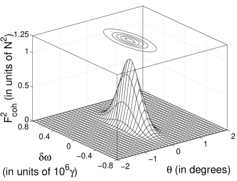
FIG. 1.: The coherent form function for one million trapped fermionic atoms at a temperature of $k_{B}T/E_{F}=1.36$.

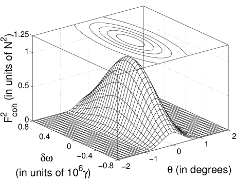
FIG. 2.: The same as Fig. 1 but at a temperature of $k_{B}T/E_{F}=0.0016$.

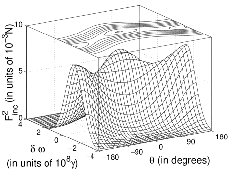
FIG. 3.: The incoherent form function for one million trapped fermionic atoms at a temperature of $k_{B}T/E_{F}=1.36$. Note that we have scaled the form function by $N$ instead of $N^{2}$.

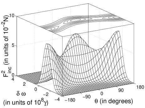
FIG. 4.: The same as Fig. 4 but at a temperature of $k_{B}T/E_{F}=0.6$.

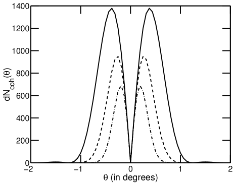
FIG. 5.: The differential coherent scattering versus angle for ten thousand trapped fermionic atoms. The solid, dashed, and dash-dotted curves represent temperatures of $k_{B}T/E_{F}=0.001$, $0.5$ and $1.0$ respectively.

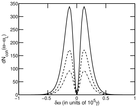
FIG. 6.: The differential coherent scattering as a function of frequency for ten thousand trapped fermionic atoms. Follows the same curve format and temperatures as Fig. 5.

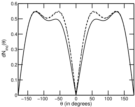
FIG. 7.: The same as Fig. 5 but for differential incoherent scattering.

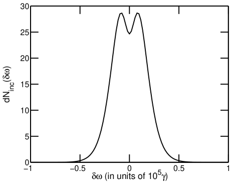
FIG. 8.: The same as Fig. 6 but for differential incoherent scattering.

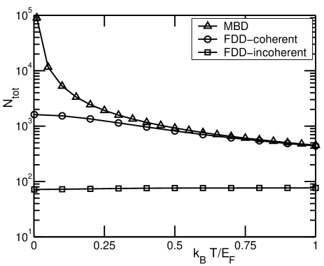
FIG. 9.: The total number of coherent and incoherent scattered photons as a function of temperature for one million trapped fermionic atoms. Coherent scattering calculated for a Maxwell-Boltzmann system is plotted as triangles. A $10$ ps laser pulse width was used in the calculations.

REFERENCES

- [1] S. Chu and C. Wieman (Eds.), special issue of J. Opt. Soc. Am. B 6, (11) (1989); S. L. Gilbert and C. E. Wieman, Opt. Photonics News, 4, 8 (1993).
- [2] M. H. Anderson, J. R. Ensher, M. R. Matthews, C. E. Wieman, and E. A. Cornell, Science 269, 198 (1995).
- [3] K. B. Davis, M. -O. Mewes, M. R. Andrews, N. J. van Druten, D. S. Durfee, D. M. Kurn, and W. Ketterle, Phys. Rev. Lett. 75, 3969 (1995).
- [4] C. C. Bradley, C. A. Sackett, J. J. Tollett, and R. G. Hulet, Phys. Rev. Lett. 75, 1687 (1995); ibid 79, 1170 (1997).
- [5] Extensive list of references exists at: http://amo.phy.gasou.edu/bec.html/bibliography.html .
- [6] B. DeMarco and D. S. Jin, Science, 285, 170 (1999).
- [7] D. S. Jin, Centennial Meeting of the American Physical Society, March 20-26, 1999, Atlanta, Georgia, Vol. 44, No. 1, FB16 8; M.-O. Mewes, G. Ferrari, F. Schreck, C. Salomon, ibid FB16 7; F. S. Cataliotti, E. A. Cornell, C. Fort, M. Inguscio, F. Martin, M. Prevedelli, L. Ricci, and G. M. Tino, Phys. Rev. A 57, 1136 (1998).
- [8] M. Lewenstein, L. You, J. Cooper, and K. Burnett, Phys. Rev. A 50, 2207 (1994); L. You, M. Lewenstein and J. Cooper, ibid 51, 4712 (1995); L. You, M. Lewenstein, J. Cooper, and R. J. Glauber, ibid 53, 329 (1996).
- [9] (a)B. Svistunov and G. Shlyapnikov, Zh. Eksp. Teor. Fiz. 97, 821 (1990) [Sov. Phys. JETP 70, 460 (1990)]; ibid. 98, 129 (1990) [71, 71 (1990)]; (b) H. D. Politzer, Phys. Rev. A 43, 6444 (1991); (c) J. Javanainen, Phys. Rev. Lett. 72, 2375 (1994); (d) O. Morice, Y. Castin, and J. Dalibard, Phys. Rev. A 51, 3896 (1995); (e) W. Zhang and D. F. Walls, ibid 49, 3799 (1994).
- [10] L. V. Hau, S. E. Harris, Z. Dutton, and C. H. Behroozi, Nature 397, 594 (1999).
- [11] L. Deng et al., Nature 398, 218 (1999).
- [12] S. Inouye et al., Science 285, 571 (1999).
- [13] (a) J. Ruostekoski and J. Javanainen, Phys. Rev. A 55, 513 (1997);(b) J. Ruostekoski and J. Javanainen, Phys. Rev. Lett. 82, 4741 (1999).
- [14] (a) W. Zhang, C. A. Sackett, and R. G. Hulet, Phys. Rev. A 60, 504 (1999);(b) J. Ruostekoski, ibid 60, R1775 (1999); (c) B. DeMarco and D. S. Jin, Phys. Rev. A 58, R4267 (1998); (d) F. Weig and W. Zwerger, cond-mat/9908176; (e) J. Ruostekoski, cond-mat/9908276.
- [15] (a) K. Helmerson, M. Xiao,D. Pritchard, International Quantum Electronics Conference 1990, book of abstracts (IEEE, New York, 1990), abstr. QTHH4; (b) Th. Busch, J. R. Anglin, J. I. Cirac, and P. Zoller, Europhys. Lett. 44, 1 (1998).
- [16] M. Lewenstein and L. You, Phys. Rev. Lett. 71, 1339 (1993).
- [17] (a) D. A. Butts and D. S. Rokhsar, Phys. Rev. A 55, 4346 (1997); (b) J. Schneider and H. Wallis, ibid 57, 1253 (1998); (c) K. Mølmer, Phys. Rev. Lett. 80, 1804 (1998).
- [18] M. Houbiers, R. Ferwerda, and H. T. C. Stoof, W. I. McAlexander, C. A. Sackett, and R. G. Hulet, Phys. Rev. A 56, 4864 (1997); A. G. K. Modawi and A. J. Leggett, J. Low Temp. Phys. Vol. 109, 625 (1997); M. A. Baranov, Yu. Kagan, and M. Yu. Kagan, Pis’ma Zh. Éksp. Teor. Fiz. 64, 273 (1996) [JETP Lett. 64, 301 (1996)]; G. M. Bruun, Y. Castin, R. Dum, and K. Burnett, Euro. J. Phys. (in the press); L. You and M. Marinescu, Phys. Rev. A 60, 2324 (1999).
- [19] W. Geist, A. Idrizbegovic, M. Marinescu, T. A. B. Kennedy, and L.You, Phys. Rev. A (in press).
- [20] K. E. Cahill and R. J. Glauber, Phys. Rev. 177, 1857, (1969).
- [21] I. S. Gradshteym and I. M. Ryzhik, Table of integrals series and products, 1039 (Academic Press, London, 1980).