Quantum stochastic resonance in driven spin-boson system with stochastic limit approximation

Abstract

After a brief review of stochastic limit approximation with spin-boson system from physical points of view, amplification phenomenon—stochastic resonance phenomenon—in driven spin-boson system is observed which is helped by the quantum white noise introduced through the stochastic limit approximation. Signal-to-noise ratio resonates at certain temperature if another noise parameter $\eta$ is chosen properly. Not only the stochastic resonance in usual sense, but also the possibilities of the new and interesting phenomena—“anti-resonance” and “double resonance”—are shown with some choices of $\eta$. The shift in frequency of the system due to the interaction with the environment—Lamb shift—has an important role in these phenomena.

I Introduction

Stochastic resonance (SR) phenomena were first discovered in connection with periodically recurrent glacial age. Since then this phenomenon has been found to occur in various fields and has been attracting wide attention. In short SR is phenomenon whereby, in contrast to common sense, added noise seems to help to amplify a signal. Let us briefly review SR phenomenon using the bistable potential model, driven by a periodic perturbation. A classical particle in a potential $V(x)$, which has two local minima, is perturbed by a periodic external force with an amplitude $\xi$ and a frequency $\Omega$ under the influence of noise (Fig. 1). If the amplitude $\xi$ is small, the particle in one of the stable states cannot go over the potential barrier to the other stable state [Fig. 1(a)], in other words, the system does not respond to the input perturbation. The addition of noise changes the situation; now the
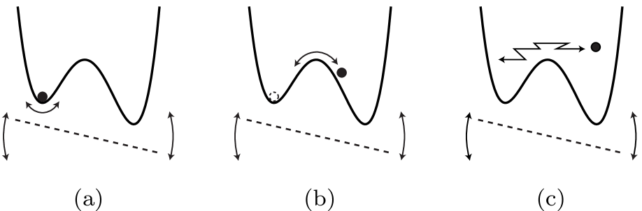
FIG. 1.: Response of a particle in a bistable potential to an external periodic perturbation with (a) too small, (b) appropriate, and (c) too strong noise. particle is kicked by the random force and can go over the barrier. However if the noise is too strong the response to the input signal may be smeared. This is because in this case the particle moves randomly irrespective of the periodicity of the perturbation [Fig. 1(c)]. However at a certain added noise strength the particle can be made to travel back and forth between the two stable state, synchronizing with periodic perturbation of frequency $\Omega$ [Fig. 1(b)]. That is the system responds to the input.

More precisely we can characterize SR as follow:

(1) The power spectrum of the response of a system to a periodic input has a main sharp peak at the input frequency $\Omega$ if the noise strength (or temperature) is chosen properly.

(2) The signal-to-noise ration (SNR) of the response resonates at a certain noise strength (or at a certain temperature).

Besides the periodicity in the emergence of glacial ages [2], SR phenomenon are widely found in nature. For example SR is found in the nerve of the flagellum of a crayfish’s tail [3] (however in this case, unlike the bistable system described above, a threshold reaction is triggered by noise). Therefore SR may be a universal concept.

In this paper we discuss SR in bistable model at the quantum level, that is quantum stochastic resonance (QSR). Of course this effect has already been widely studied [1, 4], however our particular interest is “quantum noise,” or “quantum dynamics with dissipation.” That is, we are interested in how noise is introduced into the quantum dynamics to produce QSR. This is not only important question for QSR, but it is also relevant for the understanding of several other fundamental aspects of quantum mechanics, that is the problems of relaxation, decoherence, measurement and so on. However quantum mechanics is usually written in terms of causal deterministic theory governed by unitary time evolution. It is therefore hard, in principle, to introduce the notion of “noise” or “dissipation” (with finite degrees of freedom).

In these circumstances there are several different ways to proceed. One of the most popular approaches is to introduce an “environment,” “reservoir” or “heat bath,” whose detailed specification one does not know but which has infinite degrees of freedom. The whole system (i.e. $\mbox{``system''}+\mbox{``environment''}$) is then treated in the quantum mechanical way [5, 6, 7, 8].

Through this interaction, the system exchanges energy with the environment—“dissipation”—, and then it is reasonable to assume that some kind of “noise” or “fluctuation” would appear due to some “fluctuation-dissipation relation.”

Along these lines Accardi et al. [9, 10, 11] have introduced the stochastic limit approximation (SLA) as a way to realize “quantum white noise.” The SLA is one way to deal with the van Hove limit, which is the weak coupling limit given by, $\lambda\to 0$ and time coarse-graining limit given by, $t\mapsto\tau=\lambda^{2}t$. This limit ensures that a system in a heat bath approaches canonical state [13].

As is explicitly shown in Sec. III for the spin-boson system, the spin system in the heat bath composed of bosons actually approaches the canonical state under the SLA. Furthermore, one can discuss important properties in quantum dissipative dynamics within this framework, such as the dependence on temperature of the shift in frequency of the system due to the interaction with the heat bath.

We here focus our attention on the quantum white noise introduced through the SLA, and study QSR as part of investigations of the properties of this noise. After the introduction of the model to be studied—the driven spin-boson system—in Sec. II, the SLA is briefly reviewed in Sec. III with the spin-boson system. Using this method, we discuss, in Sec. IV, QSR in the driven spin-boson system and the role of the quantum fluctuation and dissipation introduced through the SLA. Section V is devoted to concluding remarks with comments on the experimental feasibility of the phenomenon studied here. In the Appendix, we add comments on the SLA from a physical point of view.

II Driven Spin-Boson System

Here let us introduce the model—the driven spin-boson system [1, 4]—as a special case of the bistable model in Sec. I.

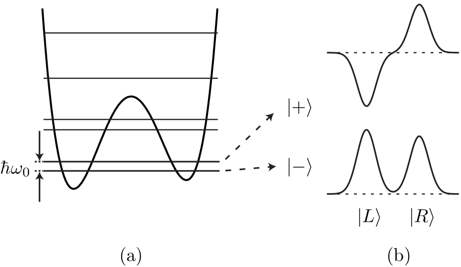
FIG. 2.: Bistable system at the quantum scale.

A Spin system

Consider the situation where the system illustrated in Fig. 2 is in a deep cold heat bath and its dynamics are ruled mainly by the lowest tunnel-splitted pair of levels $|\pm\rangle$, where thermal hopping to upper levels can be neglected. If the tunneling amplitude between the two wells is sufficiently small, we are able to consider two “localized” states, $|L\rangle$ and $|R\rangle$, which are approximately the ground states of left and right wells, respectively. Taking the set of these states as the Hilbert space basis, this system can be described by the Hamiltonian,

$$H_{S}=\frac{\epsilon}{2}\Bigl{(}|R\rangle\langle R|-|L\rangle\langle L|\Bigr{)}+\frac{\Delta}{2}\Bigl{(}|R\rangle\langle L|+|L\rangle\langle R|\Bigr{)},$$ (1)

which is essentially the spin-1/2 Hamiltonian with the parameter $\Delta$ characterizing the tunneling amplitude between the two wells, and $\epsilon$ characterizing the difference in energy between the $|L\rangle$ and $|R\rangle$ states. Hereafter, we call it the spin system. By introducing a new basis rotated by the angle $\theta=\cos^{-1}(\epsilon/\omega_{0})=\sin^{-1}(\Delta/\omega_{0})$,

$$|+\rangle=\cos\frac{\theta}{2}|R\rangle+\sin\frac{\theta}{2}|L\rangle,$$ (3)

$$|-\rangle=-\sin\frac{\theta}{2}|R\rangle+\cos\frac{\theta}{2}|L\rangle,$$ (4)

the Hamiltonian $H_{S}$ is rewritten as a diagonal form

$$H_{S}=\frac{\omega_{0}}{2}\Bigl{(}|+\rangle\langle+|-|-\rangle\langle-|\Bigr{)}.$$ (5)

The energy gap $\omega_{0}$ between the two lowest states, $|+\rangle$ and $|-\rangle$, is given by

$$\omega_{0}=\sqrt{\epsilon^{2}+\Delta^{2}}.$$ (6)

This two-level system is driven by a periodic forcing with frequency $\Omega$ and amplitude $\xi$. This applied force can be described by the perturbative Hamiltonian

$$W=\xi X\sin\Omega t$$ (7)

with the “position” operator $X$ defined by

$$X=|R\rangle\langle R|-|L\rangle\langle L|.$$ (8)

Of course, there are many other possibilities for the system driving instead of (7), e.g., $W^{\prime}=\xi(|R\rangle\langle L|+|L\rangle\langle R|)\sin\Omega t$, but we choose the perturbation (7) since it corresponds to classical SR in the bistable model.

Note that $X$ is an order parameter in discussing QSR phenomenon in Sec. IV, which measures the transitions between the states $|L\rangle$ and $|R\rangle$ under the influence of the external perturbation.

B Boson system and its interaction with the spin system

As mentioned in Sec. I, one must introduce an “environment” for the spin system to dissipate and be disturbed. The environment is chosen as a set of bosons in this paper, whose Hamiltonian is given by

$$H_{B}=\int dk\,\omega_{k}a_{k}^{\dagger}a_{k}.$$ (9)

Here, $a_{k}$ and $a_{k}^{\dagger}$ are respectively annihilation and creation operators for a boson of mode $k$ with energy $\omega_{k}>0$, and satisfy the commutation relations

$$[a_{k},a_{k^{\prime}}^{\dagger}]=\delta(k-k^{\prime}),\quad\mbox{(others)}=0.$$ (10)

The spin system interacts with the bosons via the interaction Hamiltonian

$$\lambda V=\lambda X\int dk\,(g_{k}a_{k}^{\dagger}+g_{k}^{*}a_{k}),$$ (11)

where $\lambda$ characterizes the strength of the interaction, and the structure function $g_{k}$ is a coupling of the bosons of mode $k$ with the spin system subject to the condition $\int dk\,|g_{k}|^{2}<\infty$. Note that the spin system and the boson system are coupled with the bilinear product of the spin operator $X$ and the boson operators. Although some specified choices of the coupling may result in certain outputs, the details of the microscopic Hamiltonian are not so significant for the derivation of damping dynamics. A comment on this point can be found in Sec. III B 2.

The system to be analyzed in this paper is thus given by the total Hamiltonian

$$H=H_{0}+W+\lambda V,\quad H_{0}=H_{S}+H_{B}.$$ (12)

III Stochastic Limit Approximation

In this section we briefly review the stochastic limit approximation (SLA) formulated by Accardi et al. [9, 10, 11]. For simplicity, let us consider the case where there is no external perturbation, i.e., $\xi=0$ [10, 11, 7]. The Hamiltonian of the system concerned in this section is thus

$$H_{\mathrm{S}B}=H_{0}+\lambda V.$$ (13)

We entrust the mathematical details to Ref. [9] or [11], but note that several physically important points are emphasized and added to the work in Ref. [10] and [11]. Furthermore in the appendix we add some comments on the SLA taken from slightly different point of view to that taken by Accardi et al.

A Application to spin-boson system

In the interaction picture, the time-evolution operator $U_{I}^{(\lambda)}\!(t)$ which is governed by the Hamiltonian (13) satisfies the Tomonaga–Schwinger equation

$$\frac{d}{dt}U_{I}^{(\lambda)}\!(t)=-i\lambda V_{I}(t)U_{I}^{(\lambda)}\!(t),\quad U_{I}^{(\lambda)}\!(0)=1,$$ (15)

$$V_{I}(t)=e^{iH_{0}t}Ve^{-iH_{0}t},$$ (16)

or specifically

$$\frac{d}{dt}U_{I}^{(\lambda)}\!(t)=-i\lambda\sum_{\alpha}\Bigl{(}D_{\alpha}A_{\alpha}^{\dagger}(t)+D_{\alpha}^{\dagger}A_{\alpha}(t)\Bigr{)}\,U_{I}^{(\lambda)}\!(t),$$ (17)

where $\alpha$ takes $\alpha=\{+,-,0\}$,

$$D_{\pm}=|\pm\rangle\langle\mp|,\quad D_{0}=|+\rangle\langle+|-|-\rangle\langle-|$$ (18)

are the spin system operators, and

$$A_{\pm}(t)=-\frac{\Delta}{\omega_{0}}\int dk\,g^{*}_{k}a_{k}e^{-i(\omega_{k}\pm\omega_{0})t},$$ (20)

$$A_{0}(t)=\frac{\epsilon}{\omega_{0}}\int dk\,g^{*}_{k}a_{k}e^{-i\omega_{k}t}$$ (21)

are the boson system operators. The SLA is prescribed in the Tomonaga–Schwinger equation (17) by rescaling time as $t\mapsto\tau=\lambda^{2}t$,

$$\frac{d}{d\tau}U_{I}^{(\lambda)}\!(\tau/\lambda^{2})= -i\frac{1}{\lambda}\sum_{\alpha}\Bigl{(}D_{\alpha}A_{\alpha}^{\dagger}(\tau/\lambda^{2})+D_{\alpha}^{\dagger}A_{\alpha}(\tau/\lambda^{2})\Bigr{)}\,$$ (23)

$$\qquad{}\times U_{I}^{(\lambda)}\!(\tau/\lambda^{2}),$$

and then the weak coupling limit $\lambda\rightarrow 0$ is taken (i.e., the van Hove limit [12, 13]). As proved in Ref. [9] or [11], there exist the limits

$$\frac{1}{\lambda}A_{\alpha}(\tau/\lambda^{2})\rightarrow b_{\alpha}(\tau),\quad\frac{1}{\lambda}A_{\alpha}^{\dagger}(\tau/\lambda^{2})\rightarrow b_{\alpha}^{\dagger}(\tau),$$ (24)

$$U_{I}^{(\lambda)}\!(\tau/\lambda^{2})\rightarrow U_{I}(\tau),$$ (25)

and formally

$$\frac{d}{d\tau}U_{I}(\tau)=-i\sum_{\alpha}\Bigl{(}D_{\alpha}b^{\dagger}_{\alpha}(\tau)+D_{\alpha}^{\dagger}b_{\alpha}(\tau)\Bigr{)}\,U_{I}(\tau).$$ (26)

In this limit, the boson operators $b_{\alpha}(\tau)$ and $b_{\alpha}^{\dagger}(\tau)$ satisfy the commutation relations [10, 11]

$$[b_{-}(\tau),b_{-}^{\dagger}(\tau^{\prime})]=2\gamma\delta(\tau-\tau^{\prime}),\quad(\mbox{others})=0$$ (27)

with

$$\gamma=\left(\frac{\Delta}{\omega_{0}}\right)^{2}J(\omega_{0}),$$ (28)

$$J(\omega)=\pi\int dk\,|g_{k}|^{2}\delta(\omega_{k}-\omega).$$ (29)

For comments on these limits from a physical point of view, see the Appendix. The commutation relations (27) allow one reasonably to call $b_{\alpha}(\tau)$ and $b_{\alpha}^{\dagger}(\tau)$ “quantum white noise,” and the Tomonaga–Schwinger equation (26) the “quantum Langevin equation.” The correlation time is vanishingly small. However at the same time, we should be careful to note that equation (26) is ill-defined. Fortunately, however, noticing the commutators [10, 11]

$$[b_{\pm}(\tau),U_{I}(\tau)]=-i\left(\frac{\Delta}{\omega_{0}}\right)^{2}\gamma(\mp\omega_{0})D_{\pm}U_{I}(\tau),$$ (31)

$$[b_{0}(\tau),U_{I}(\tau)]=-i\left(\frac{\epsilon}{\omega_{0}}\right)^{2}\gamma(0)D_{0}U_{I}(\tau)$$ (32)

with

$$\gamma(\omega)=J(\omega)-iI(\omega),\quad I(\omega)=\frac{1}{\pi}{\cal P}\!\int d\omega^{\prime}\,\frac{J(\omega^{\prime})}{\omega^{\prime}-\omega},$$ (33)

one can evaluate the evolutions of some physically important quantities. For example, for the special initial state density operator

$$\rho=\rho_{S}\otimes\rho_{B},\quad\rho_{B}=|0\rangle\langle 0|$$ (34)

(i.e., the spin system and the boson system are uncorrelated and the boson system is in the ground state at $\tau=0$), the equations for the spin system operators defined by

$$D_{\alpha}(\tau)=\mathop{\mathrm{t}r}\nolimits_{B}\!\left(\rho_{B}\,e^{iH_{\mathrm{S}B}\tau/\lambda^{2}}D_{\alpha}e^{-iH_{\mathrm{S}B}\tau/\lambda^{2}}\right)$$ (35)

can be obtained as

$$\frac{d}{d\tau}D_{\pm}(\tau)=-(\gamma\mp i\omega_{R})D_{\pm}(\tau),$$ (37)

$$\frac{d}{d\tau}D_{0}(\tau)=-2\gamma D_{0}(\tau)-2\gamma,$$ (38)

which give the exponentially decaying dynamics

$$D_{\pm}(\tau)=D_{\pm}e^{-(\gamma\mp i\omega_{R})\tau},$$ (40)

$$D_{0}(\tau)=(D_{0}+1)e^{-2\gamma\tau}-1.$$ (41)

Here $\omega_{R}$ is the renormalized frequency

$$\omega_{R}=\omega_{0}/\lambda^{2}-\sigma=\tilde{\omega}_{0}-\sigma,$$ (42)

where the frequency shift $\sigma$ emerges due to the interaction

$$\sigma=\left(\frac{\epsilon}{\omega_{0}}\right)^{2}\Bigl{(}I(\omega_{0})-I(-\omega_{0})\Bigr{)}.$$ (43)

Note that $\mathop{\mathrm{t}r}_{B}$ denotes the trace over the boson-degrees of freedom. This is the procedure for “partial trace.” It reduces the effects of the interaction between the spin system and the boson environment to the spectral function $J(\omega)$ defined in Eq. (29). The damping coefficient $\gamma$ in Eq. (28) and the frequency shift $\sigma$ in Eq. (43) with Eq. (33) are both given in terms of $J(\omega)$.

It is also possible to evaluate $\gamma$ and $\sigma$ for the boson environment at finite temperature $T$

$$\rho_{B}=e^{-\beta H_{B}}/\mathop{\mathrm{t}r}\nolimits_{B}e^{-\beta H_{B}}$$ (44)

by using the TFD technique [14], for example. Here $\beta=1/k_{B}T$ with $k_{B}$ being the Boltzmann constant. In this case, one obtains

$$D_{\pm}(\tau)=D_{\pm}e^{-(\gamma^{\beta}\mp i\omega_{R}^{\beta})\tau},$$ (46)

$$D_{0}(\tau)=\left(D_{0}+\frac{\gamma}{\gamma^{\beta}}\right)e^{-2\gamma^{\beta}\tau}-\frac{\gamma}{\gamma^{\beta}}$$ (47)

with the temperature affected parameters

$$\gamma^{\beta}=\left(\frac{\Delta}{\omega_{0}}\right)^{2}J^{\beta}\!(\omega_{0}),$$ (49)

$$\omega_{R}^{\beta}=\omega_{0}/\lambda^{2}-\sigma^{\beta}=\tilde{\omega}_{0}-\sigma^{\beta},$$ (50)

$$\sigma^{\beta}=\left(\frac{\epsilon}{\omega_{0}}\right)^{2}\Bigl{(}I^{\beta}\!(\omega_{0})-I^{\beta}\!(-\omega_{0})\Bigr{)},$$ (51)

and the functions

$$J^{\beta}\!(\omega)=J(\omega)\coth\frac{1}{2}\beta\omega,$$ (53)

$$I^{\beta}\!(\omega)=\frac{1}{\pi}{\cal P}\!\int d\omega^{\prime}\,\frac{J^{\beta}\!(\omega^{\prime})}{\omega^{\prime}-\omega}.$$ (54)

The damping coefficient $\gamma^{\beta}$ and the frequency shift $\sigma^{\beta}$ are obtained from $\gamma$ and $\sigma$, respectively, by replacing the spectral function $J(\omega)$ with the temperature modified one $J^{\beta}\!(\omega)$.

Notice that the long-time limits of the operators $D_{0}(\tau)\rightarrow-\tanh(\beta\omega_{0}/2)$ and $D_{\pm}(\tau)\rightarrow 0$ are both c-numbers (or unit operators of the spin system multiplied by c-numbers). This means that the spin system approaches some unique state irrespective of the initial state $\rho_{S}$. In fact, the averages of any spin system operators, which are composed of $D_{\alpha}(\tau)$, approach unique values. One can further confirm that the long-time limit of the state of the spin system is nothing but the thermal state at the temperature $T$. Taking averages of $D_{\alpha}(\tau)$ with some arbitrary initial state $\rho_{S}$, one obtains the matrix elements of the system density operator defined by

$$\rho_{S}(\tau)=\mathop{\mathrm{t}r}\nolimits_{B}\rho(\tau),$$ (55)

$$\rho(\tau)=e^{-iH_{\mathrm{S}B}\tau/\lambda^{2}}\rho\,e^{iH_{\mathrm{S}B}\tau/\lambda^{2}}.$$ (56)

Their dynamics are immediately obtained from the equations (44), and their long-time limits are given by

$$\langle-|\rho_{S}(\tau)|+\rangle=\langle D_{+}(\tau)\rangle\rightarrow 0,$$ (58)

$$\langle\pm|\rho_{S}(\tau)|\pm\rangle =\frac{1}{2}\Bigl{(}1\pm\langle D_{0}(\tau)\rangle\Bigr{)}$$ (60)

$$\rightarrow\frac{e^{\mp\beta\omega_{0}/2}}{e^{\beta\omega_{0}/2}+e^{-\beta\omega_{0}/2}},$$

which are equivalent to

$$\rho_{S}(\tau)\rightarrow e^{-\beta H_{S}}/\mathop{\mathrm{t}r}\nolimits_{S}e^{-\beta H_{S}},$$ (61)

i.e., the system approaches the thermal equilibrium state at temperature $T$ through decoherence (58). Here $\mathop{\mathrm{t}r}\nolimits_{S}$ denotes the trace over the spin-degrees of freedom.

B Comments from physical points of view

1 Orders of parameters

It is important to clarify the order of magnitude of the parameters. In this formalism, one considers that the new time $\tau$ is physical and that, if they are measured in this macroscopic time, the parameters of the spin system should have some meaningful values, e.g., $\omega_{R}^{\beta}$ or $\tilde{\omega}_{0}$, instead of $\omega_{0}$, should be finite. On the other hand, the time scales of the boson system should be measured in the microscopic time $t$. This can be seen in the emergence of the delta function in Eq. (27). This is due to the coarse-graining in time, $t\mapsto\tau=\lambda^{2}t\,(\lambda\rightarrow 0)$. It reflects the fact that characteristic time scales of the boson system, like the correlation time for example, are vanishingly small when measured in the macroscopic time. That is they are negligible when compared to the characteristic times of the spin system, such as $1/\tilde{\omega}_{0}$ for example. This is the situation which occurs in the stochastic limit.

As for the temperature, the physically interesting situation is where the temperature $T$ is such that $\beta\omega_{0}$ has some finite value, which is contained in $\gamma^{\beta}$ and $\sigma^{\beta}$ through $J^{\beta}\!(\omega_{0})$ [see Eqs. (47) and (51)] and in the thermal equilibrium distribution (60). That is, the rescaled temperature $\tilde{T}=T/\lambda^{2}$ should be finite.

2 Choice of the coupling

In this paper, the spin-boson system is coupled through the specific choice of the coupling, in particular, the choice $X$. Of course, there are many other possibilities, such as $V=(|R\rangle\langle L|+|L\rangle\langle R|)\int dk\,(g_{k}a_{k}^{\dagger}+g_{k}^{*}a_{k})$, but they all result in the same damping dynamics (44) except for the prefactors $(\Delta/\omega_{0})^{2}$ and $(\epsilon/\omega_{0})^{2}$ in the definitions of $\gamma^{\beta}$ and $\sigma^{\beta}$ in Eqs. (49) and (51). [One has to notice, however, that the special choice of the interaction $V=(|+\rangle\langle+|-|-\rangle\langle-|)\int dk\,(g_{k}a_{k}^{\dagger}+g_{k}^{*}a_{k})$ gives the special situation $\gamma^{\beta}=0$, which is also included in Eqs. (44). The possibility of $\sigma^{\beta}=0$ also exists for some special choices of $V$.] From a semi-phenomenological point of view, Eqs.(44) are sufficient for the description of experiments. Knowledge of the parameters $\tilde{\omega}_{0}$, $\gamma^{\beta}$, and $\sigma^{\beta}$ from an experiment would enable one to predict the dynamical development of any quantities. Details of the microscopic Hamiltonian would not have much effect on the macroscopic behavior.

IV Quantum Stochastic Resonance

Now let us discuss QSR in the driven spin-boson system (12) with the SLA. By observing the response of the system to the external perturbation (7) through the dynamics of the “position” operator

$$X(\tau)=\mathop{\mathrm{t}r}\nolimits_{B}\!\left(\rho_{B}\,e^{iH\tau/\lambda^{2}}Xe^{-iH\tau/\lambda^{2}}\right),$$ (62)

which measures the transitions of the system between the left state $|L\rangle$ and the right state $|R\rangle$, we see an amplification of the input external perturbation with the addition of noise.

The Tomonaga–Schwinger equation is now

$$\frac{d}{dt}U_{I}^{(\lambda)}\!(t)=-i\Bigl{(}\lambda V_{I}(t)+W_{I}(t)\Bigr{)}\,U_{I}^{(\lambda)}\!(t),\quad U_{I}^{(\lambda)}\!(0)=1,$$ (64)

$$W_{I}(t)=\xi\left[\frac{\epsilon}{\omega_{0}}D_{0}-\frac{\Delta}{\omega_{0}}\left(D_{+}e^{i\omega_{0}t}+D_{-}e^{-i\omega_{0}t}\right)\right]\sin\Omega t,$$ (65)

and along the same lines as in Sec. III, the SLA ($t\mapsto\tau=\lambda^{2}t$, $\lambda\rightarrow 0$) is taken to give the “quantum Langevin equation”

$$\frac{d}{d\tau}U_{I}(\tau)= -i\sum_{\alpha}\Bigl{(}D_{\alpha}b_{\alpha}^{\dagger}(\tau)+D_{\alpha}^{\dagger}b_{\alpha}(\tau)\Bigr{)}U_{I}(\tau)$$ (69)

$${}-i\tilde{\xi}\left[\frac{\epsilon}{\omega_{0}}D_{0}-\frac{\Delta}{\omega_{0}}\left(D_{+}e^{i\tilde{\omega}_{0}\tau}+D_{-}e^{-i\tilde{\omega}_{0}\tau}\right)\right]$$

$$\qquad{}\times\sin(\tilde{\Omega}\tau)U_{I}(\tau).$$

Note that the parameters are rescaled as $\tilde{\omega}_{0}=\omega_{0}/\lambda^{2}$, $\tilde{\Omega}=\Omega/\lambda^{2}$, and $\tilde{\xi}=\xi/\lambda^{2}$ according to time rescaling, and are assumed to take physical values if measured in the macroscopic time. The equations of the spin system operators $D_{\alpha}(\tau)$ are then given by

$$\frac{d}{d\tau}D_{\pm}(\tau)=-(\gamma^{\beta}\mp i\omega_{R}^{\beta})D_{\pm}(\tau)$$ (71)

$$\qquad{}\pm 2i\tilde{\xi}\left(\frac{\epsilon}{\omega_{0}}D_{\pm}(\tau)+\frac{1}{2}\frac{\Delta}{\omega_{0}}D_{0}(\tau)\right)\sin\tilde{\Omega}\tau,$$ (72)

$$\frac{d}{d\tau}D_{0}(\tau)=-\gamma^{\beta}D_{0}(\tau)-\gamma$$ (73)

$$\qquad{}+2i\tilde{\xi}\frac{\Delta}{\omega_{0}}\Bigl{(}D_{+}(\tau)-D_{-}(\tau)\Bigr{)}\sin\tilde{\Omega}\tau.$$ (74)

These are, however, difficult to solve exactly, so we rely upon the perturbation method and assume that the external perturbation is weak. (One is interested here in SR phenomenon, i.e., amplification of weak inputs with the help of noise.) The solutions up to $O(\tilde{\xi}/\tilde{\omega}_{0})$ or $O(\xi/\omega_{0})$ are thus obtained for long times $\tau\gg 1/\gamma^{\beta}$ as

$$D_{\pm}(\tau)\rightarrow \mp\frac{i}{2}\tilde{\xi}\frac{\Delta}{\omega_{0}}\tanh\frac{1}{2}\beta\omega_{0}\left[\frac{1}{(\omega_{R}^{\beta}-\tilde{\Omega})\pm i\gamma^{\beta}}e^{\pm i\tilde{\Omega}\tau}\right.$$ (77)

$$\qquad\left.{}-\frac{1}{(\omega_{R}^{\beta}+\tilde{\Omega})\pm i\gamma^{\beta}}e^{\mp i\tilde{\Omega}\tau}\right],$$

$$D_{0}(\tau)\rightarrow-\tanh\frac{1}{2}\beta\omega_{0},$$ (78)

and $X(\tau)$, by combining these solutions, as

$$X(\tau)=\frac{\epsilon}{\omega_{0}}D_{0}(\tau)-\frac{\Delta}{\omega_{0}}\Bigl{(}D_{+}(\tau)+D_{-}(\tau)\Bigr{)}$$ (79)

$$\qquad{}\rightarrow-\frac{\epsilon}{\omega_{0}}\tanh\frac{1}{2}\beta\omega_{0}{}+\frac{\xi}{\omega_{0}}A^{\beta}\!(\tilde{\Omega})\sin\!\left(\tilde{\Omega}\tau-\phi^{\beta}\!(\tilde{\Omega})\right).$$ (80)

(81)

Here the amplitude $A^{\beta}\!(\tilde{\Omega})$ and the phase delay $\phi^{\beta}\!(\tilde{\Omega})$ are given, respectively, by

$$A^{\beta}\!(\tilde{\Omega})=\frac{2(\Delta/\omega_{0})^{2}\tilde{\omega}_{0}\omega_{R}^{\beta}\tanh(\beta\omega_{0}/2)}{\sqrt{\Bigl{(}(\omega_{R}^{\beta})^{2}-\tilde{\Omega}^{2}+(\gamma^{\beta})^{2}\Bigr{)}^{2}+\Bigl{(}2\gamma^{\beta}\tilde{\Omega}\Bigr{)}^{2}}}$$ (82)

and

$$\tan\phi^{\beta}\!(\tilde{\Omega})=\frac{2\gamma^{\beta}\tilde{\Omega}}{(\omega_{R}^{\beta})^{2}-{\tilde{\Omega}}^{2}+(\gamma^{\beta})^{2}}.$$ (83)

Responding to the input perturbation, $X(\tau)$ oscillates around the thermal equilibrium state with the frequency of the perturbation $\tilde{\Omega}$.

Let us define the signal-to-noise ratio (SNR) $R^{\beta}\!(\tilde{\Omega})$ by

$$R^{\beta}\!(\tilde{\Omega})=|A^{\beta}\!(\tilde{\Omega})|/(\gamma^{\beta}\!/\tilde{\omega}_{0}),$$ (84)

and study its dependence on the temperature. If this resonates at any certain temperature we conclude SR exists in this model. In the following, we show the analyses for two specific choices of the spectral function $J(\omega)$, as examples. One choice is

$$J(\omega)=\left\{\begin{array}[]{ll}\displaystyle\eta\omega&\displaystyle(0<\omega<\Lambda)\\ \displaystyle\\ \displaystyle\eta\Lambda&\displaystyle(\omega>\Lambda)\end{array}\right.,$$ (86)

called here the “Ohmic case” [Fig. 3(b)], and the other is

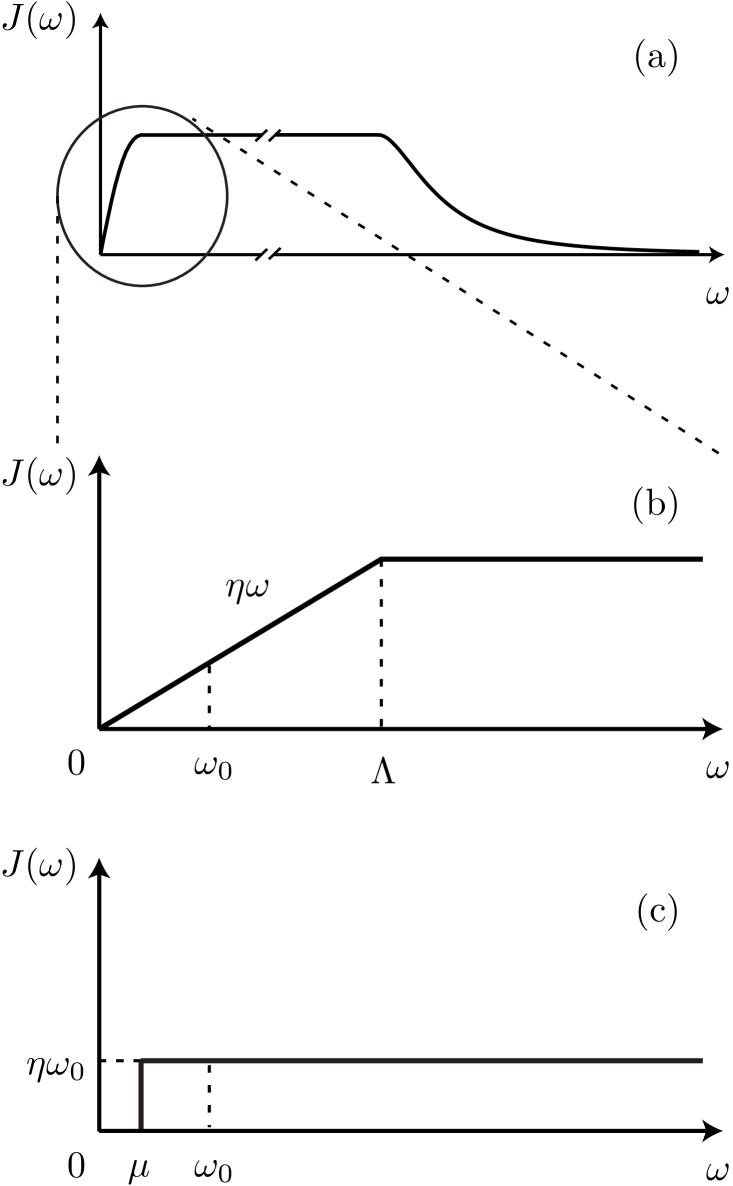
FIG. 3.: Functional form of (a) physically realistic, (b) “Ohmic case,” and (c) “constant case” spectral function $J(\omega)$.

$$J(\omega)=\left\{\begin{array}[]{ll}\displaystyle 0&\displaystyle(0<\omega<\mu)\\ \displaystyle\\ \displaystyle\eta\omega_{0}&\displaystyle(\omega>\mu)\end{array}\right.,$$ (87)

called the “constant case” [Fig. 3(c)]. Although a physically realistic spectral function $J(\omega)$ may have a cutoff at high frequency $\Lambda_{C}$ as sketched in Fig. 3(a), it may be reasonable to consider that $\Lambda_{C}$ can be infinitely large compared to the characteristic frequency of the spin system $\omega_{0}$ in the stochastic limit situation. We hence adopt the model spectral functions given by Eqs. (86) and (87) and illustrated in Figs. 3(b) and (c). Their names come from the functional forms in the regions around “on-shell” $\omega=\omega_{0}$ which are assumed to be the regions $0<\omega<\Lambda$ and $\mu<\omega$ for each case. Note that $J(\omega_{0})$, and hence $\gamma^{\beta}$ given by Eq. (49), have the same value for both cases, and the dimensionless parameter $\eta$ controls its magnitude, i.e., the noise strength. The difference between the two cases manifests itself in the temperature dependence of the frequency shift $\sigma^{\beta}$ given by Eq. (51) (Fig. 4). Note further that the function $I^{\beta}\!(\omega)$ defined by the dispersion relation (54) does not converge with the model spectral functions (84). Since the asymptotic behaviors of $J^{\beta}\!(\omega)$ in these models are constant as $\omega\to\infty$, one has to apply a subtracted form to the dispersion relation. After a subtraction at $\omega=\omega_{1}$, this becomes

$$I^{\beta}\!(\omega)=I^{\beta}\!(\omega_{1})+\frac{\omega-\omega_{1}}{\pi}{\cal P}\!\int d\omega^{\prime}\,\frac{J^{\beta}\!(\omega^{\prime})-J^{\beta}\!(\omega_{1})}{(\omega^{\prime}-\omega_{1})(\omega^{\prime}-\omega)}.$$ (88)

Choosing the subtraction point as $\omega_{1}=0$, one gets a convergent integral,

$$I^{\beta}\!(\omega)=I^{\beta}\!(0)+\frac{\omega}{\pi}{\cal P}\!\int d\omega^{\prime}\,\frac{J^{\beta}\!(\omega^{\prime})}{\omega^{\prime}(\omega^{\prime}-\omega)}.$$ (89)

From Eqs. (54) and (89), the frequency shift is given by

$$\sigma^{\beta}=\left(\frac{\epsilon}{\omega_{0}}\right)^{2}\frac{2\omega_{0}}{\pi}{\cal P}\!\int d\omega^{\prime}\,\frac{J^{\beta}\!(\omega^{\prime})}{\omega^{\prime 2}-\omega_{0}^{2}}.$$ (90)

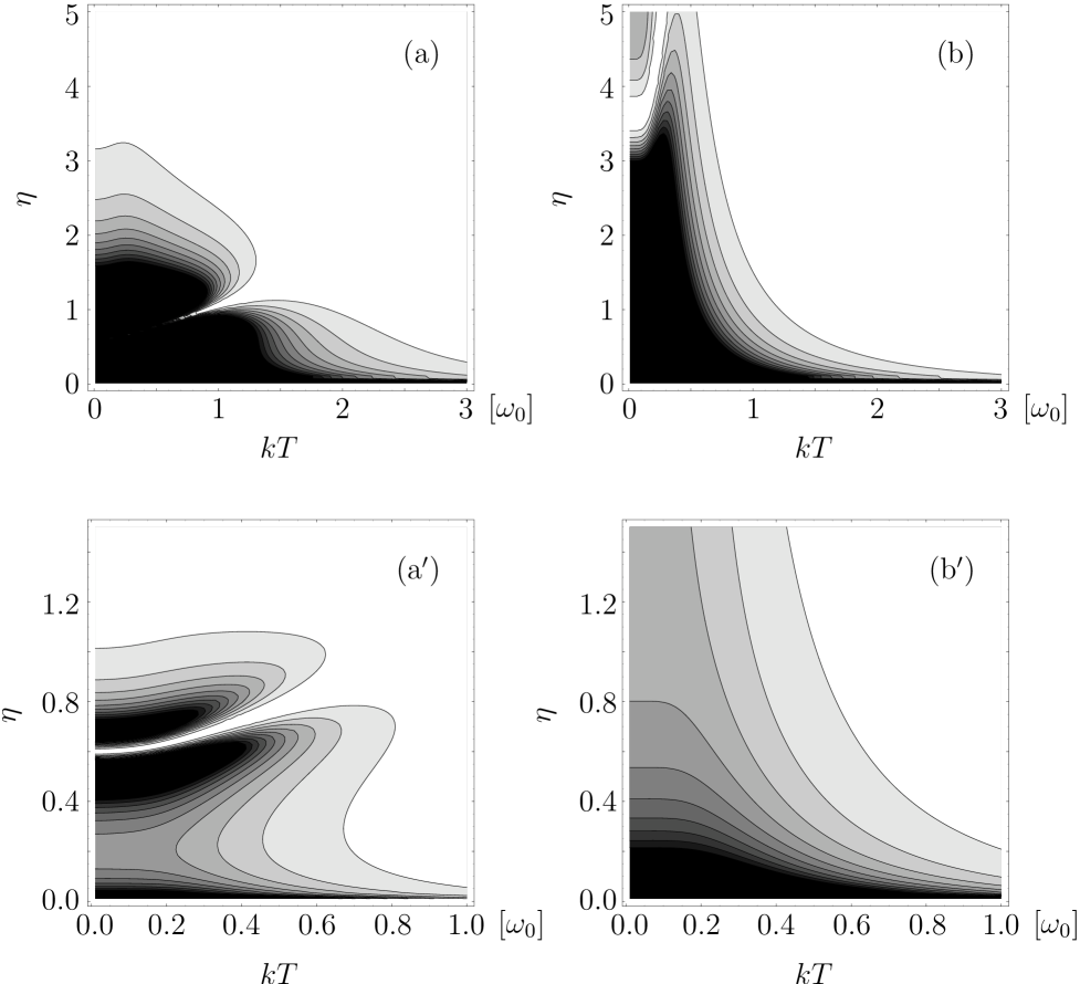
There are two important parameters concerning the environment or the noise, i.e., the temperature $T$ and
FIG. 4.: Schematic forms of the frequency shift for (a) “Ohmic case” and (b) “constant case.” FIG. 5.: Temperature- and $\eta$-dependence of SNR for (a) “Ohmic case” and (b) “constant case” with $\Omega=0.10\omega_{0}$, $\Lambda=2.0\omega_{0}$, $\mu=0.50\omega_{0}$, and $\Delta/\omega_{0}=0.35$. (a^′) and (b^′) are enlarged versions of (a) and (b), respectively. Darker grays correspond to larger $R^{\beta}\!(\tilde{\Omega})$. the noise strength $\eta$. In Fig. 5, the SNRs $R^{\beta}\!(\tilde{\Omega})$ for both cases are shown in the $\eta$-$T$ plane. One may realize at first sight that SNR depends deeply on the choice of $J^{\beta}\!(\omega)$, namely, on the temperature dependence of the frequency shift $\sigma^{\beta}$. The temperature dependences of the SNRs are shown in Fig. 6(a) for the “Ohmic case” with $\eta=0.59$, and in Fig. 6(b) for the “constant case” with $\eta=3.5$. maximum values are seen at around the temperature $kT\sim 0.3\omega_{0}$ for both cases, that is, SR occurs. Roughly speaking, these maximum points correspond to the minima of the denominator in the right hand side of Eq. (82). One has to notice, however, that this does not occur for all $\eta$: for some $\eta$ it occurs, and for others it does not. And beyond these two possibilities, one can find some strange phenomena. See Fig. 6(a^′), where $\eta$ is chosen as $\eta=0.65$ for the “ohmic case,” and Fig. 6(b^′), where $\eta=4.5$ for the “constant case.” There exist temperatures where the system does not respond. We may call this “anti-resonance.” It occurs when the frequency shift $\sigma^{\beta}$ coincides with the system frequency $\tilde{\omega}_{0}$. See the numerator of the amplitude $A^{\beta}\!(\tilde{\Omega})$. And see Fig. 6(a^′′) with $\eta=0.70$ for the “ohmic case” and Fig. 6(b^′′) with $\eta=15$ for the “constant case,” where the SNRs have two peaks, i.e., “double resonance.” The second maximum comes from the overlapping effect of a negatively decreasing factor $\omega_{R}^{\beta}$ beyond its zero point and a positively decreasing Planck distribution. And it does not correspond to a genuine SR. It has no counterpart in classical systems. The behavior of the frequency shift $\sigma^{\beta}$ may FIG. 6.: Temperature-dependence of SNR for “Ohmic case” with (a) $\eta=0.59$, (a^′) $\eta=0.65$, and (a^′′) $\eta=0.70$, and for “constant case” with (b) $\eta=3.5$, (b^′) $\eta=4.5$, and (b^′′) $\eta=15$.
be the key to these phenomena.

V Summary

QSR in the driven spin-boson system is discussed with quantum white noise introduced through the SLA. The SLA is a framework which can be used to describe the van Hove limit, which ensures the approach of system in a thermal environment to the thermal equilibrium state. SNRs versus noise parameters—temperature $T$ and the noise strength $\eta$—are studied with two model spectral functions $J(\omega)$. The occurrence of SR depends on the choice of $\eta$. For some $\eta$ the system does not resonate, for other values it does, and a new phenomenon—anti-resonance and double resonance— is observed. The temperature dependence of the frequency shift of the system $\sigma^{\beta}$ due to the interaction with the environment—Lamb shift—may be the key to these phenomena. In this sense, QSR owes its existence to a quantum effect, which is different from the classical SR, where random force itself is important. To understand this point, this system should be studied in the crossover area between the quantum and classical regimes. This work is now in progress.

It should further be emphasized that the analysis here is from the microscopic view point, not from a semi-phenomenological viewpoint. In the latter there is no criterion which would tell us how to incorporate the damping coefficient $\gamma^{\beta}$ and the frequency shift $\sigma^{\beta}$ into the phenomenological equation properly. Here the damping dynamics is obtained from the fundamental microscopic Hamiltonian underneath the theory.

Finally, let us mention experimental situations for the present analysis.

(1) The physical time is not $t$ but $\tau$. Experimental data should be compared with the theoretical predictions from the analysis in this paper in the macroscopic time $\tau$.

(2) It is very difficult in general to prepare precise quantum mechanical initial conditions experimentally. Fortunately, however, SNR is obtained from the stationary behavior of the system at large times $\tau\gg 1/\gamma^{\beta}$, and is irrespective of the initial condition.

(3) It is possible to control $J(\omega)$ in the cavity QED experiment. In fact, the life-time of the unstable state of an atom can be successfully controlled by changing the modes of the electromagnetic field, i.e., by changing $J(\omega)$. This means that it may be possible to observe SNRs with different choices of $J(\omega)$ in the cavity QED.

There may be technical difficulties to overcome, but it may be possible to observe experimentally the phenomena predicted here. This would also be an experimental verification of SLA itself.

Here we briefly describe SLA from a physical point of view. Introducing a generalized rescaled time as

$$t\mapsto\tau=\lambda^{\nu}t,\quad\nu>0,$$ (91)

one has the Tomonaga–Schwinger equation

$$\frac{d}{d\tau}U_{I}^{(\lambda)}\!(\tau/\lambda^{\nu})= -i\frac{1}{\lambda^{\nu-1}}\sum_{\alpha}\Bigl{(}D_{\alpha}A_{\alpha}^{\dagger}(\tau/\lambda^{\nu})$$ (93)

$$\qquad{}+D_{\alpha}^{\dagger}A_{\alpha}(\tau/\lambda^{\nu})\Bigr{)}\,U_{I}^{(\lambda)}\!(\tau/\lambda^{\nu}).$$

We require that the rescaled operators $A_{\alpha}$, $A_{\alpha}^{\dagger}$ should satisfy the commutation relations with respect to the rescaled time $\tau$. It is easily shown that the possible choices are only of the form $A_{\alpha}(\tau/\lambda^{\nu})/\lambda^{\nu/2}$ and that the non-trivial commutation relation is

$$\left[\frac{1}{\lambda^{\nu/2}}A_{-}(\tau/\lambda^{\nu}),\frac{1}{\lambda^{\nu/2}}A_{-}^{\dagger}(\tau^{\prime}/\lambda^{\nu})\right]$$ (94)

$$\qquad=2\left(\frac{\Delta}{\omega_{0}}\right)^{2}\left[J(\omega_{0})+i\lambda^{\nu}J^{\prime}(\omega_{0})\frac{\partial}{\partial\tau}+\cdots\right]$$ (95)

$$\qquad\qquad\qquad\qquad\qquad{}\times\frac{1}{2\pi}\int_{-\omega_{0}/\lambda^{\nu}}^{\infty}\!dx\,e^{-ix(\tau-\tau^{\prime})},$$ (96)

while the others vanish. If the first and higher derivatives of the spectral function $J^{(n)}(\omega_{0})\,(n=1,2,\ldots)$ do not have singularities, one can safely neglect all terms other than $J(\omega_{0})$ from the expansion. This corresponds simply to the choice of diagonal singularity, i.e., only the boson mode $\omega_{k}=\omega_{0}$ contributes to the damping coefficient in the scaling limit $\lambda\to 0$.

From the above considerations, it is convenient to rewrite Eq. (93) as

$$\frac{d}{d\tau}U_{I}^{(\lambda)}\!(\tau/\lambda^{\nu})$$ (97)

$$\qquad=-i\lambda^{1-\nu/2}\sum_{\alpha}\biggl{(}D_{\alpha}\frac{1}{\lambda^{\nu/2}}A_{\alpha}^{\dagger}(\tau/\lambda^{\nu})$$ (98)

$$\qquad\qquad\qquad{}+D_{\alpha}^{\dagger}\frac{1}{\lambda^{\nu/2}}A_{\alpha}(\tau/\lambda^{\nu})\biggr{)}\,U_{I}^{(\lambda)}\!(\tau/\lambda^{\nu}).$$ (99)

Thus, one can see that, in the limit $\lambda\to 0$, (1) the right hand side of Eq. (97) vanishes in the case of “under” SLA ($\nu<2$), while (2) it diverges in the case of “over” SLA ($\nu>2$), and (3) it has a formal limit in the case of “critical” SLA ($\nu=2$). Therefore the only meaningful result occurs in the $\nu=2$ case.

REFERENCES

- [1] For reviews, see L. Gammaitoni, P. Hänggi, P. Jung, and F. Marchesoni, Rev. Mod. Phys. 70, 223 (1998).
- [2] R. Benzi, G. Parisi, A. Sutera, and A. Vulpiani, Tellus 34, 10 (1982).
- [3] J. K. Douglass, L. Wilkens, E. Pantazelou, and F. Moss, Nature 365, 337 (1993).
- [4] For reviews, see M. Grifoni and P. Hänggi, Phys. Rep. 304, 229 (1998). They discussed the system described by Eq. (12), based on the approach quoted in the paper by Leggett et al. [A. J. Leggett et al., Rev. Mod. Phys. 59, 1 (1987)]. They also obtained the non-linear response of an order parameter to an applied field, and their works have given us many stimulations. But it is hard to get result analytically except for some special parameter.
- [5] R. P. Feynman and F. L. Vernon, Ann. Phys. 24, 118 (1963); R. P. Feynman and A. R. Hibbs, Quantum Mechanics and Path Integrals (McGraw-Hill, New York, 1965).
- [6] A. O. Caldeira and A. J. Leggett, Ann. Phys. 149, 374 (1983); 153, 445(E) (1984); Physica 121A, 587 (1983); 130A, 374(E) (1985).
- [7] A. J. Leggett, S. Chakravarty, A. T. Dorsey, M. P. A. Fisher, A. Garg, and W. Zwerger, Rev. Mod. Phys. 59, 1 (1987).
- [8] U. Weiss, Quantum Dissipative Systems, Vol. 2 of Series in Modern Condensed Matter Physics (World Scientific, Singapore, 1993).
- [9] L. Accardi, A. Frigerio, and Y. G. Lu, Commun. Math. Phys. 131, 537 (1990); L. Accardi, J. Gough, and Y. G. Lu, Rep. Math. Phys. 36, 155 (1995).
- [10] L. Accardi, S. V. Kozyrev, and I. V. Volovich, Phys. Rev. A 56, 2557 (1997).
- [11] L. Accardi, Y. G. Lu, and I. V. Volovich, Quantum Theory and Its Stochastic Limit (Oxford University Press, London, in press).
- [12] L. van Hove, Physica 21, 517 (1955).
- [13] E. B. Davies, Commun. Math. Phys. 39, 91 (1974).
- [14] H. Umezawa, Advanced Field Theory: Micro, Macro, and Thermal Physics (American Institute of Physics, New York, 1993).