Abstract

Intermediate states interpolating coherent states and Pegg-Barnett phase states are investigated using the ladder operator approach. These states reduce to coherent and Pegg-Barnett phase states in two different limits. Statistical and squeezing properties are studied in detail.

1 Introduction and Motivation

Since Stoler et al introduced the binomial states (BS) in 1985 [1], the so-called intermediate states interpolating two fundamental states of radiation fields have attracted much interests in quantum optics [1-13]. The BS is defined as a linear superposition of number states in an $(M+1)$-dimensional subspace

$$|\eta,\,M\rangle=\sum_{n=0}^{M}\left[\beta_{n}^{M}(\eta)\right]^{\frac{1}{2}}|n\rangle,$$ (1.1)

where $\eta$ is a real parameter satisfying $0<\eta<1$, and

$$\beta_{n}^{M}(\eta)={M\choose n}\eta^{n}(1-\eta)^{M-n}$$ (1.2)

is the binomial distribution with probability $\eta$. In the limits $\eta\to 1$ and $\eta\to 0$, BS reduce to number states $|1,\,M\rangle=|M\rangle$ and $|0,\,M\rangle=|0\rangle$, respectively. In a different limit of $M\to\infty,\ \eta\to 0$ with $\eta M=\alpha^{2}$ fixed ($\alpha$ real constant) $|\eta,\,M\rangle$ reduce to the coherent states with real amplitude $\alpha$. In this sense, BS are the intermediate number-coherent states. The notion of BS was also generalized to the multinomial [6] and negative multinomial states [6, 7], hypergeometric states [8], Pólya states [9], intermediate number-squeezed states [10, 11] and the number-phase states [12], as well as its $q$-deformation [13].

In a previous paper [10] one of the authors presented a ladder operator formalism of BS, namely, BS satisfy the following eigenvalue equation

$$\left(\sqrt{\eta}N+\sqrt{1-\eta}J^{+}_{M}\right)|M,\eta\rangle=\sqrt{\eta}M|M,\eta\rangle,$$ (1.3)

where $J^{+}_{M}=\sqrt{M-N}\,a\,$ is the raising operator of su(2) via its Holstein-Primakoff realization. We also proposed the generalized BS by replacing $J^{+}_{M}$ with a linear combinatio of $J^{+}_{M}$ and $J^{-}_{M}\equiv(J^{+}_{M})^{\dagger}$ which are the intermediate number-squeezed states. From this approach we learn that (1) the parameter $\eta$ plays the role of controlling two different limits and (2) the limit to coherent states is essentially the contraction of Lie algebra su(2) to the oscillator algebra: $\sqrt{\eta}J_{M}^{+}\to\alpha a$ in the limit $\eta\to 0$ and $M\to\infty$ with $\eta M=\alpha^{2}$. So in the ladder operator approach of an intermediate state we can us su(2) generators to control the coherent state limit.

In this letter we shall pay our attention to the intermediate states between coherent states and the Pegg-Barnett (PB) phase states, which, to our knowledge, are not considered in the literature. We shall generalize the ladder operator approach of BS to these intermediate coherent-phase(PB) states (ICPS). Above discussion on BS suggest us proposing the following eigenvalue equation

$$\left(\sqrt{\eta}\mbox{e}^{\hat{\Phi}}+\sqrt{1-\eta}J_{M}^{+}\right)|M,\eta,\rho\rangle=\rho|M,\eta,\rho\rangle.$$ (1.4)

Here $0<\eta<1$ is real as in the BS case, and $\rho$ is eigenvalue to be determined. The operator $\mbox{e}^{\hat{\Phi}}$ is the exponential PB phase operator defined by [14]

$$\mbox{e}^{\hat{\Phi}}|\theta_{m}\rangle=e^{\theta_{m}}|\theta_{m}\rangle$$ (1.5)

on the PB phase state

$$|\theta_{m}\rangle=\frac{1}{\sqrt{M+1}}\sum_{n=0}^{M}\exp{(in\theta_{m})}|n\rangle,\ \ \ \ \theta_{m}=\frac{2\pi m}{M+1}+\theta_{0},$$ (1.6)

where $\theta_{0}$ is a real constant.

We shall solve the equation (1.4) in next section an then discuss its limits to coherent and PB phase states in Sec.3. The photon statistics and the squeezing properties are investigated in detail in Sec.4. Sec.5 is a concluding remark. We note that these states are shown to be finite superposition of Fock states and in principle can be experimentally fabricated, as reported recently in [16]

2 Intermediate coherent-phase(PB) states

Equation (1.4) is an eigenvalue equation of an $(M+1)\times(M+1)$ matrix, so it has $M+1$ eigenvalues and corresponding eigenstates. To solve it, we expand the state $|M,\eta,\rho\rangle$ in terms of the number state

$$|M,\eta,\rho\rangle=\sum_{n=0}^{M}C_{n}|n\rangle.$$ (2.1)

Inserting (2.1) into (1.4) and using the following relations [15]

$$\mbox{e}^{\hat{\Phi}}|n\rangle=|n-1\rangle\ \ \ \ (n\neq 0),\ \ \ \ \mbox{e}^{\hat{\Phi}}|0\rangle=e^{i(M+1)\theta_{0}}|M\rangle,$$ (2.2)

we obtain the following equations

$$\sqrt{\eta}C_{0}e^{i(M+1)\theta_{0}}=\rho C_{M},$$ (2.3)

$$\left(\sqrt{1-\eta}\sqrt{n(M-n+1)}+\sqrt{\eta}\right)C_{n}=\rho C_{n-1}\ \ \ \ (n=1,\cdots,M).$$ (2.4)

From (2.4) we have

$$C_{n}=\frac{\rho^{n}}{F(n)!}C_{0}\ \ \ \ (n=1,\cdots,M),$$ (2.5)

where

$$F(n)=\sqrt{1-\eta}\sqrt{n(M-n+1)}+\sqrt{\eta},$$ (2.6)

$$F(n)!=F(n)F(n-1)\cdots F(1),\ \ \ F(0)!\equiv 1.$$ (2.7)

Relation (2.5) with $n=M$ must be consistent with the condition (2.3), namely,

$$\sqrt{\eta}C_{0}e^{i(M+1)\theta_{0}}=\frac{\rho^{M+1}}{F(M)!}C_{0},$$ (2.8)

which leads to $M+1$ distinct eigenvalues ($C_{0}\neq 0$)

$$\rho_{m}=\left(\sqrt{\eta}F(M)!\right)^{\frac{1}{M+1}}e^{i\theta_{m}},\ \ \ \ 0\leq m\leq M,$$ (2.9)

where $\theta_{m}$ is the same as in Eq.(1.6). The normalization constant $C_{0}$ can be easily determined as

$$C_{0}=\left[\sum_{n=0}^{M}\left(\frac{[\sqrt{\eta}F(M)!]^{\frac{n}{M+1}}}{F(n)!}\right)^{2}\right]^{-\frac{1}{2}}.$$ (2.10)

Substituting (2.9) into (2.1) we finally find the ICPS (we write $|M,\eta,\rho_{m}\rangle\equiv|M,\eta,\theta_{m}\rangle$

$$|M,\eta,\theta_{m}\rangle=\sum_{n=0}^{M}D_{n}^{M}(\eta e^{i\theta_{m}n}|n\rangle,$$ (2.11)

$$D_{n}^{M}(\eta)=\left(\sum_{n=0}^{M}\left(\frac{[\sqrt{\eta}F(M)!]^{\frac{n}{M+1}}}{F(n)!}\right)^{2}\right)^{-\frac{1}{2}}\frac{\left(\sqrt{\eta}F(M)!\right)^{\frac{n}{M+1}}}{F(n)!}$$ (2.12)

Here we have written $e^{i\theta_{m}n}$ separately for convenience in later use.

It is interesting that using the identity method in [15] these states can also be written as the form of a displacement operator acting on the vacuum state

$$|M,\eta,\theta_{m}\rangle=C_{0}\exp_{M}\left(\frac{[\sqrt{\eta}F(M)!]^{\frac{1}{M+1}}\sqrt{N}}{F(N)}\,a^{\dagger}\right)|0\rangle,$$ (2.13)

where $\exp_{M}(x)=\sum_{n=0}^{M}x^{n}/n!$ is the finite exponential function.

The parameter $\theta_{0}$ ($0\leq\theta<2\pi$) has clear physical meaning: it reflects the time development of ICPS. This can be seen from $e^{-iHt}|M,\eta,\theta_{m}\rangle=|M,\eta,\theta_{m}-\omega t\rangle$, where $H=\omega(N+1/2)$ is the Hamiltonian of the single mode radiation field. In next section we shall see that in the coherent limit, $\theta_{0}$ do gives the imaginary part of amplitude of limiting coherent states which reflects the time evolution of coherent states.

3 Limits to PB phase states and coherent states

We first consider the limit $\eta\to 1$. It is easy to see that

$$\frac{\left[\sqrt{\eta}F(M)!\right]^{\frac{n}{M+1}}}{F(n)!}\to 1,\ \ \ C_{0}\to\left(\sum_{n=0}^{M}1\right)^{-1/2}=\frac{1}{\sqrt{M+1}}$$ (3.1)

So

$$|M,\eta,\theta_{m}\rangle\to\frac{1}{\sqrt{M+1}}\sum_{n=0}^{M}e^{i\theta_{m}n}|n\rangle\equiv|\theta_{m}\rangle.$$ (3.2)

We arrive at the PB phase states.

In a different limit: $M\to\infty$, $\eta\to 0$ keeping $\eta(M/\alpha)^{M+1}=\beta$ a finite constant ($\alpha$ is a real constant), we will get the coherent states. In this limit, $F(n)\to\sqrt{nM}$, $F(M)!\to M!$ and

$$(M+1)^{\frac{1}{M+1}}\sim 1,\ \ \ M\sim M+1\ \ \ \ \mbox{for $M\to\infty$}.$$ (3.3)

We then have

$$\frac{[\sqrt{\eta}F(M)!\,]^{\frac{n}{M+1}}}{F(n)!}=\frac{1}{\sqrt{n!}}\left[\lim_{\scriptsize\begin{array}[]{c}M\to\infty\\ \eta\to 0\end{array}}\left(\sqrt{\eta M^{M+1}}\right)^{\frac{1}{M+1}}\lim_{M+1\to\infty}\frac{[(M+1)!]^{\frac{1}{M+1}}}{M+1}\right]^{n}.$$ (3.4)

By making use of the following limit formula

$$\lim_{M+1\to\infty}\frac{[(M+1)!]^{\frac{1}{M+1}}}{M+1}=\frac{2}{e},$$ (3.5)

we have

$$\frac{[\sqrt{\eta}F(M)!]^{\frac{n}{M+1}}}{F(n)!}\to\frac{1}{\sqrt{n!}}\left(\frac{2}{e}\alpha\right)^{n}.$$ (3.6)

In this limit, $C_{0}$ and $\theta_{m}$ reduce to

$$C_{0}\to\exp{\left(-\frac{2\alpha^{2}}{e^{2}}\right)},\ \ \ \theta_{m}\to\theta_{0}.$$ (3.7)

From (3.6) and (3.7) we obtain the coherent state limit

$$|M,\eta,\theta_{m}\rangle\to\left|\frac{2\alpha}{e}e^{i\theta_{0}}\right\rangle\equiv\exp{\left(-\frac{2\alpha^{2}}{e^{2}}\right)}\sum_{n=0}^{\infty}\frac{\left(\frac{2\alpha}{e}e^{i\theta_{0}}\right)^{n}}{\sqrt{n!}}|n\rangle.$$ (3.8)

We note that $M+1$ different ICPS reduce to the same coherent state due to $\theta_{m}\to\theta_{0}$ for all $m$.

We also remark that, similarly to the BS, the intermediate coherent-(PB)phase states degenerate to the vacuum state in the limit $\eta\to 0$.

4 Nonclassical properties

4.1 Photon statistics

Mandel’s $Q$-factor characterizing sub(super)-Poissonian distribution is obtained as

$$Q(M,\eta)=\frac{\langle\Delta N^{2}\rangle}{\langle N\rangle}-1=\frac{\sum_{n=0}^{M}[D^{M}_{n}(\eta)]^{2}n^{2}-\left[\sum_{n=0}^{M}[D^{M}_{n}(\eta)]^{2}n\right]^{2}}{\sum_{n=0}^{M}[D^{M}_{n}(\eta)]^{2}n}-1.$$ (4.1)

If $Q<0\ (>0)$, the field is of sub(super)-Poissonian. $Q=0$ corresponds to the Poissonian statistics. We note that $Q(M,\eta)$ is independent of the parameter $\theta_{m}$ and therefore it reflects the photon statistics of all $M+1$ state $|M,\eta,\theta_{m}\rangle$.

Fig.1. is a plot of $Q(M,\eta)$ as a function of $\eta$ for different values of $M$ $(1,2,\cdots,7)$. We find that the field on ICPS is of sub-Poissonian in the case $M=1$ except for the end point $\eta=0$. For the cases $M=2,3$, the field becomes super-Poissonian first from the Poissonian statistics at $\eta=0$, and then the sub-Poissonian. The range of the sub-Poissonian statistics for $M=2$ is wider than that for $M=3$. When $M=4$, the fields are of super-Poissonian except for two end points $\eta=0,1$, which correspond Poissonian. Finally, if $M>4$, the fields are super-Poissonian except for the starting point $\eta=0$. We here note that the $Q$-factor of the PB phase states is $Q(M,0)=(M-4)/6$, which correspond to the right ends of the $Q$ factor.

4.2 Squeezing effect

Define the coordinate $x$ and the momentum $p$ as

$$x=\frac{1}{\sqrt{2}}(a^{\dagger}+a),\ \ \ p=\frac{i}{\sqrt{2}}(a^{\dagger}-a).$$ (4.2)

Then their variances $(\Delta x)^{2}\equiv\langle x^{2}\rangle-\langle x\rangle^{2}$ and $(\Delta p)^{2}\equiv\langle p^{2}\rangle-\langle p\rangle^{2}$ are obtained as

$$(\Delta x)^{2} = \frac{1}{2}+\sum_{n=0}^{M}nD^{M}_{n}(\eta)^{2}+\cos(2\theta_{m})\sum_{n=0}^{M-2}\sqrt{(n+1)(n+2)}D^{M}_{n}(\eta)D^{M}_{n+2}(\eta)$$

$$-2\left(\cos(\theta_{m})\sum_{n=0}^{M-1}\sqrt{n+1}D^{M}_{n}(\eta)D^{M}_{n+1}(\eta)\right)^{2},$$

$$(\Delta p)^{2} = \frac{1}{2}+\sum_{n=0}^{M}nD^{M}_{n}(\eta)^{2}-\cos(2\theta_{m})\sum_{n=0}^{M-2}\sqrt{(n+1)(n+2)}D^{M}_{n}(\eta)D^{M}_{n+2}(\eta)$$ (4.3)

$$+2\left(\sin(\theta_{m})\sum_{n=0}^{M-1}\sqrt{n+1}D^{M}_{n}(\eta)D^{M}_{n+1}(\eta)\right)^{2}.$$

If $(\Delta x)^{2}<1/2$ (or $(\Delta p^{2})<1/2$), we say the quadrature $x$ (or $p$) is squeezed.

We first note that $(\Delta x)^{2}$ and $(\Delta p)^{2}$ are related with each other by the following relation

$$(\Delta x)^{2}_{\theta_{m}}=(\Delta p)^{2}_{\theta_{m}\pm\pi/2}.$$ (4.4)

So hereafter we only consider the quadrature $(\Delta x)^{2}$. Then it is obvious that $(\Delta x)^{2}$ is a $\pi$-periodic function of $\theta_{m}$ and it is symmetric with respect to $\theta_{m}=\pi/2$.

Figures 2 shows how $(\Delta x)^{2}$ depends on parameters $M$, $\eta$ and $\theta_{m}$, respectively. From these plots we find that

1. When $\theta_{m}=\pi/2$. In this case the quadrature $x$ is not squeezed at the point $\eta=0$, which corresponds to the vacuum state. Then, with the increase of $\eta$, it becomes squeezed drastically until the maximum of squeezing (minimum of $(\Delta x)^{2}$) is reached. By further increasing $\eta$, the squeezing becomes weaker and weaker until it disappears for a large enough $\eta_{0}$. The squeezing range $0<\eta<\eta_{0}$ depends on $M$: the larger $M$, the wider the squeezing range and the smaller $(\Delta x)^{2}$.

2. Dependence on $\theta_{m}$. Since $(\Delta x)^{2}$ is symmetric with respect to $\theta_{m}=\pi/2$, so we only plot $\theta_{m}\leq\pi/2$ part in Fig.2. We see that, with the decreas (or increase) of $\theta_{m}$ form $\pi/2$, the squeezing becomes weaker and weaker and the squeezing range $0<\eta<\eta_{0}$ for a fixed $\theta_{m}$ becomes narrower and narrower, until squeezing disappears for small (or large) enough $\theta_{m}$.

5 Conclusion

In this paper we have introduced the intermediate coherent-phase(PB) states by ladder operator approach and investigated their nonclassical properties. As the intermediate states, these states interpolate between the coherent states and the PB phase states and reduce to them in two different limits. They also exhibit strong nonclassical properties such as sub-Poissonian statistics and squeezing effect in considerable ranges of parameters involved.

Finally, we point out that, as a finite superposition of Fock states, these states in principle can be experimentally fabricated, as reported recently [16].

Figure 1: The Mandel’s $Q$-factor $Q(M,\eta)$ as a funtion of $\eta$, for different $M=1,\cdots,7$.

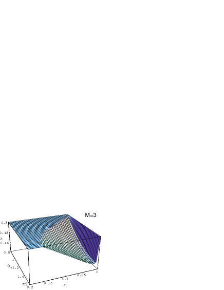
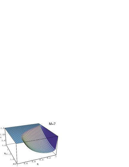
Figure 2: Variance $\langle\Delta x^{2}\rangle\equiv X$ as a function of $\eta$ and $\theta_{m}$ for $M=3,\,7$.

References

- [1] D. Stoler, B. E. A. Saleh and M. C. Teich Opt. Acta. 32 (1985) 34.
- [2] C. T. Lee, Phys. Rev. 31A (1985) 121.
- [3] A. V. Barranco and J. Roversi, Phys. Rev. 50A (1994) 5233.
- [4] G. Dattoli, J. Gallardo and A. Torre, J. Opt. Soc. Am. 2B (1987) 185.
-
[5]
A. Joshi and R. R. Puri,
J. Mod. Opt. 36 (1989) 557;
M. E. Moggin, M. P. Sharma and A. Gavrielides, ibid. 37 (1990) 99. - [6] H. C. Fu and R. Sasaki, J. Math. Phys. 38 (1997) 3968. quant-ph/961002.
- [7] H. C. Fu and R. Sasaki, J. Jap. Phys. Soc. 66 (1997) 1989, quant-ph/961002.
- [8] H. C. Fu and R. Sasaki, J. Math. Phys. 38 (1997) 2154, quant-ph/961002
- [9] H. C. Fu, J. Phys. 30A (1997) L83.
- [10] H. C. Fu and R. Sasaki, J. Phys. 29A (1996) 5637
- [11] B. Baseia, A. F. de Lima and A. J. da Silva, Mod. Phys. Lett. 9B (1995) 1673.
- [12] B. Baseia, A. F. de Lima and G. C. Marques, Phys. Lett. 204A (1995) 1
- [13] H. Y. Fan and S. C. Jing, Phys. Rev. 50A (1994) 1909.
- [14] D. T. Pegg and S. M. Barnett, Europhys. Lett. 6 (1988) 6; Phys. Rev. A 39 (1989) 1665; S. M. Barnet and D. T. Pegg, J. Mod. Phys. 36 (198) 7; Phys. Rev. 50A 190.
- [15] See, for example, H. C. Fu and R. Sasaki, J. Phys. 29A (1997) 4049.
- [16] J. Janszky, P. Domokos, S. Szabo and Adam Phys. Rev. 51A (1995) 4191.