Quantum perfect correlations and
Hardy’s nonlocality theorem

Abstract

In this paper the failure of Hardy’s nonlocality proof for the class of maximally entangled states is considered. A detailed analysis shows that the incompatibility of the Hardy equations for this class of states physically originates from the fact that the existence of quantum perfect correlations for the three pairs of two-valued observables $(D_{11},D_{21})$, $(D_{11},D_{22})$, and $(D_{12},D_{21})$ [in the sense of having with certainty equal (different) readings for a joint measurement of any one of the pairs $(D_{11},D_{21})$, $(D_{11},D_{22})$, and $(D_{12},D_{21})$], necessarily entails perfect correlation for the pair of observables $(D_{12},D_{22})$ [in the sense of having with certainty equal (different) readings for a joint measurement of the pair $(D_{12},D_{22})$]. Indeed, the set of these four perfect correlations is found to satisfy the CHSH inequality, and then no violations of local realism will arise for the maximally entangled state as far as the four observables $D_{ij}$, $i,j=1$ or $2$, are concerned. The connection between this fact and the impossibility for the quantum mechanical predictions to give the maximum possible theoretical violation of the CHSH inequality is pointed out. Moreover, it is generally proved that the fulfillment of all the Hardy nonlocality conditions necessarily entails a violation of the resulting CHSH inequality. The largest violation of this latter inequality is determined.

Key words: perfect correlation, maximally entangled state, local realism, Hardy’s nonlocality theorem, Bell’s inequality.

1 Introduction

A very remarkable feature of Hardy’s nonlocality proof [1] is that it goes through for any entangled states of a $2\times 2$ system except those which are maximally entangled such as the singlet state of two spin-$\frac{1}{2}$ particles. At first sight this might appear rather surprising in view of the fact that maximally entangled states yield the maximum violation predicted by quantum mechanics of the Clauser-Horne-Shimony-Holt (CHSH) inequality [2]. Referring himself to this failure, Hardy states that [1], “the reason for this is that the proof relies on a certain lack of symmetry that is not available in the case of a maximally entangled state.” Indeed, it has been found [1, 3-6] that the set of Hardy equations (see Eqs. (8a)-(8d) below) upon which the nonlocality contradiction is constructed is incompatible for the case of maximal entanglement in the sense that for this case the fulfillment of all three conditions (8a), (8b), and (8c) precludes the fulfillment of condition (8d), and vice versa. From a mathematical point of view this is the reason for the failure, and this would be the end of the story.

In this paper I would like to account for this failure from a somewhat different perspective which provides a fuller mathematical understanding of the structure of Hardy’s theorem. This will allow us to gain some insight into the physical cause of the inability of completely entangled states to produce a Hardy-type nonlocality contradiction. So, after introducing in Sec. 2 some general results concerning the conditions needed to achieve perfect correlations for $2\times 2$ systems, in Sec. 3 it will be shown that the fulfillment of all three conditions (8a)-(8c) in the case of a maximally entangled state necessarily entails perfect correlation between the two measurement outcomes (one for each particle) obtained in any one of the four possible combinations of joint measurements ($D_{1k},D_{2l}$), $k,l=1$ or $2$, one might actually perform on both particles, where $D_{1k}$ and $D_{2l}$ are single-particle observables associated with particles 1 and 2, respectively. However, as we shall see, the CHSH inequality is fulfilled for such maximal-entanglement-induced perfect correlations, and, thereby, no violations of local realism will arise for the maximally entangled state as long as the four observables $D_{1k}$ and $D_{2l}$ involved in the CHSH inequality make conditions (8a), (8b), and (8c) hold. Indeed, the fulfillment of the CHSH inequality for such perfect correlations means that all of them can be consistently explained in terms of a local hidden-variable model (see, for instance, Appendix D in Ref. 7 for an explicit example of such a model that accounts for the perfect correlations of two spin-$\frac{1}{2}$ particles in the singlet state). This is ultimately the physical reason why Hardy’s nonlocality argument does not work for the maximally entangled case. Moreover, as will become clear, the failure of Hardy’s argument for the maximally entangled state is, interestingly enough, closely related to the fact that the quantum mechanical predictions cannot give the maximal possible theoretical violation of the CHSH inequality. In Sec. 4, the general case of less-than-maximally entangled state is considered, and it is shown how the fulfillment of all the Hardy conditions (8a)-(8d) necessarily leads to a violation of the resulting CHSH inequality. The largest extent of this violation is determined. Finally, in Sec. 5, examples are given illustrating the fact that maximally entangled states yield the maximum quantum mechanical violation of the CHSH inequality, while this inequality is necessarily obeyed for such states if these latter are constrained to satisfy the conditions (8a), (8b), and (8c).

2 Perfect correlations for $\mathbf{2\times 2}$ systems

Hardy’s nonlocality proof involves an experimental set-up of the Einstein-Podolsky-Rosen-Bohm type [8, 9]: two correlated particles 1 and 2 fly apart in opposite directions from a common source such that each of them subsequently impinges on an appropriate measuring device which can measure either one of two physical observables at a time—$D_{11}$ or $D_{12}$ for (the apparatus measuring) particle 1, and $D_{21}$ or $D_{22}$ for (the one measuring) particle 2. Conventionally, it is supposed that the measurement of each one of these observables gives the possible outcomes “$+1$” and “$-1$” (this is the case that arises, for example, in the realistic situation [10] in which a photon is detected behind a two-channel polarizer, with the value $+1$ $(-1)$ assigned to detections corresponding to the transmitted (reflected) photon), so that we shall generally assume that the operators associated with such observables are of the form, $\hat{D}_{ij}=\left|d_{ij}^{+}\right\rangle\left\langle d_{ij}^{+}\right|-\left|d_{ij}^{-}\right\rangle\left\langle d_{ij}^{-}\right|$, with $i,j=1$ or $2$, and where $\left\{\left|d_{ij}^{+}\right\rangle,\left|d_{ij}^{-}\right\rangle\right\}$ constitutes an orthonormal basis for the Hilbert space pertaining to particle $i$. On the other hand, according to the Schmidt decomposition theorem (see, for instance, Ref. 11 for a recent account of this topic), we can always write the quantum pure state of our two-particle system as a sum of two biorthogonal terms

$$\left|\eta\right\rangle=c_{1}\left|u_{1}\right\rangle\left|u_{2}\right\rangle+c_{2}\left|v_{1}\right\rangle\left|v_{2}\right\rangle,$$ (1)

for some suitably chosen orthonormal basis $\{\left|u_{i}\right\rangle,\left|v_{i}\right\rangle\}$ for particle $i$, with the real coefficients $c_{1}$ and $c_{2}$ satisfying the relation $c_{1}^{2}+c_{2}^{2}=1$. Now, by expressing the eigenvectors $\left|d_{ij}^{+}\right\rangle$ and $\left|d_{ij}^{-}\right\rangle$ in terms of the basis vectors $\left|u_{i}\right\rangle$ and $\left|v_{i}\right\rangle$

$$\left|d_{ij}^{+}\right\rangle =e^{i\alpha_{ij}}\cos\beta_{ij}\left|u_{i}\right\rangle+e^{i\gamma_{ij}}\sin\beta_{ij}\left|v_{i}\right\rangle,$$ (2a)

$$\left|d_{ij}^{-}\right\rangle =-e^{-i\gamma_{ij}}\sin\beta_{ij}\left|u_{i}\right\rangle+e^{-i\alpha_{ij}}\cos\beta_{ij}\left|v_{i}\right\rangle,$$ (2b)

one can evaluate the quantum probability distributions $P_{\eta}(D_{1k}=m,D_{2l}=n)$, with $m,n=\pm 1$ and $k,l=1$ or $2$, that a joint measurement of the observables $D_{1k}$ and $D_{2l}$ on particles 1 and 2, respectively, gives the outcomes $D_{1k}=m$ and $D_{2l}=n$ when the particles are described by the state vector (1). These are given by

$$P_{\eta}(D_{1k} =+1,D_{2l}=+1)$$

$$=c_{1}^{2}\cos^{2}\beta_{1k}\cos^{2}\beta_{2l}+c_{2}^{2}\sin^{2}\beta_{1k}\sin^{2}\beta_{2l}$$

$$\;\;\;\;+\tfrac{1}{2}c_{1}c_{2}\cos\delta_{1k2l}\sin 2\beta_{1k}\sin 2\beta_{2l}\,,$$ (3a)

$$P_{\eta}(D_{1k} =-1,D_{2l}=-1)$$

$$=c_{1}^{2}\sin^{2}\beta_{1k}\sin^{2}\beta_{2l}+c_{2}^{2}\cos^{2}\beta_{1k}\cos^{2}\beta_{2l}$$

$$\;\;\;\;+\tfrac{1}{2}c_{1}c_{2}\cos\delta_{1k2l}\sin 2\beta_{1k}\sin 2\beta_{2l}\,,$$ (3b)

$$P_{\eta}(D_{1k} =+1,D_{2l}=-1)$$

$$=c_{1}^{2}\cos^{2}\beta_{1k}\sin^{2}\beta_{2l}+c_{2}^{2}\sin^{2}\beta_{1k}\cos^{2}\beta_{2l}$$

$$\;\;\;\;-\tfrac{1}{2}c_{1}c_{2}\cos\delta_{1k2l}\sin 2\beta_{1k}\sin 2\beta_{2l}\,,$$ (3c)

$$P_{\eta}(D_{1k} =-1,D_{2l}=+1)$$

$$=c_{1}^{2}\sin^{2}\beta_{1k}\cos^{2}\beta_{2l}+c_{2}^{2}\cos^{2}\beta_{1k}\sin^{2}\beta_{2l}$$

$$\;\;\;\;-\tfrac{1}{2}c_{1}c_{2}\cos\delta_{1k2l}\sin 2\beta_{1k}\sin 2\beta_{2l}\,,$$ (3d)

where $\delta_{1k2l}=\delta_{1k}-\delta_{2l}$, with $\delta_{1k}=\gamma_{1k}-\alpha_{1k}$ and $\delta_{2l}=\alpha_{2l}-\gamma_{2l}$. Of course, the above probabilities add up to unity

$$\sum_{m,n=\pm 1}P_{\eta}(D_{1k}=m,D_{2l}=n)=1\,.$$ (4)

We will note at this point that for the special case in which $\left|c_{1}\right|=\left|c_{2}\right|=2^{-1/2}$ (i.e., when state (1) happens to be totally entangled), the following two equalities, $P_{\eta}(D_{1k}=+1,D_{2l}=+1)=P_{\eta}(D_{1k}=-1,D_{2l}=-1)$ and $P_{\eta}(D_{1k}=+1,D_{2l}=-1)=P_{\eta}(D_{1k}=-1,D_{2l}=+1)$, hold true. Now, the expectation value of the product of the measurement outcomes of $D_{1k}$ and $D_{2l}$ is defined (in an obvious notation) as

$$E_{\eta}(D_{1k},D_{2l})=P_{\eta}^{++}+P_{\eta}^{--}-P_{\eta}^{+-}-P_{\eta}^{-+}.$$ (5)

Substituting expressions (3a)-(3d) into Eq. (5) gives

$$E_{\eta}(D_{1k},D_{2l})=\cos 2\beta_{1k}\cos 2\beta_{2l}+2c_{1}c_{2}\cos\delta_{1k2l}\sin 2\beta_{1k}\sin 2\beta_{2l}\,.$$ (6)

(Note, incidentally, that for either $c_{1}=0$ or $c_{2}=0$ (i.e., for product states) the quantum correlation function (6) factorizes with respect to the parameters $\beta_{1k}$ and $\beta_{2l}$, and consequently it will be unable to yield a violation of Bell’s inequality.) In general the correlation function (6) takes on values in the range between $-1$ and $+1$. We are interested in determining the conditions under which this function attains its extremal values $\pm 1$. By direct inspection of Eq. (6) it follows at once that whenever we have $\beta_{1k}=n_{1k}\pi/2$ and $\beta_{2l}=n_{2l}\pi/2$ ($n_{1k},n_{2l}=0,\pm 1,\pm 2,\ldots\,\,$), perfect correlations happen for any state of the form (1) irrespective of the values of $c_{1}$ and $c_{2}$. This corresponds to the case that the operators $\hat{D}_{1k}$ and $\hat{D}_{2l}$ have eigenvectors that arise from the Schmidt decomposition of the entangled state (see Eq. (1)). For this case the operators $\hat{D}_{1k}$ and $\hat{D}_{2l}$ take the form $\hat{D}_{1k}=\mu_{1k}\left|u_{1}\right\rangle\left\langle u_{1}\right|+\eta_{1k}\left|v_{1}\right\rangle\left\langle v_{1}\right|$ and $\hat{D}_{2l}=\mu_{2l}\left|u_{2}\right\rangle\left\langle u_{2}\right|+\eta_{2l}\left|v_{2}\right\rangle\left\langle v_{2}\right|$ (with $\mu_{1k}$, $\eta_{1k}$, $\mu_{2l}$, and $\eta_{2l}$ being sign factors fulfilling $\mu_{1k}\eta_{1k}=\mu_{2l}\eta_{2l}=-1$), and then, from the very structure of the state vector (1), it is apparent that a measurement of $D_{1k}$ on particle 1 will uniquely determine the outcome of a measurement of $D_{2l}$ on particle 2, and vice versa. On the other hand, for the case in which $c_{1},c_{2}\neq 0$, and $\beta_{1k}\neq n_{1k}\pi/2$, $\beta_{2l}\neq n_{2l}\pi/2$, it follows that in order for the correlation function (6) to take on its extremal values $\pm 1$ it is necessary that, (i) the state (1) be maximally entangled, and (ii) $\delta_{1k2l}=n_{1k2l}\pi$, $n_{1k2l}=0,\pm 1,\pm 2,\ldots$ . Indeed, whenever the equality $2c_{1}c_{2}\cos\delta_{1k2l}=\mp 1$ holds, Eq. (6) reduces to

$$E_{\eta}(D_{1k},D_{2l})=\cos 2(\beta_{1k}\pm\beta_{2l})\,,$$ (7)

which attains the value $+1$ or $-1$ for $\beta_{1k}\pm\beta_{2l}=m_{1k2l}\pi/2$, $m_{1k2l}=0,\pm 1$, $\pm 2,\ldots$ .

3 Hardy’s nonlocality conditions: implications for the maximally entangled case

In terms of joint probabilities, a generic two-particle state $\left|\eta\right\rangle$ of the form (1) will show Hardy-type nonlocality contradiction if the following four conditions are simultaneously fulfilled for the state $\left|\eta\right\rangle$ [1, 3-6],

$$P_{\eta}(D_{11}=-1,D_{21}=-1) \,=\,0\,,$$ (8a)

$$P_{\eta}(D_{11}=+1,D_{22}=+1) \,=\,0\,,$$ (8b)

$$P_{\eta}(D_{12}=+1,D_{21}=+1) \,=\,0\,,$$ (8c)

$$P_{\eta}(D_{12}=+1,D_{22}=+1) \,>\,0\,.$$ (8d)

Taking into account the aforementioned equalities, $P_{\eta}(D_{1k}=+1,D_{2l}=+1)=P_{\eta}(D_{1k}=-1,D_{2l}=-1)$ and $P_{\eta}(D_{1k}=+1,D_{2l}=-1)=P_{\eta}(D_{1k}=-1,D_{2l}=+1)$, which are valid only in the case that the state $\left|\eta\right\rangle$ is maximally entangled, it is immediate to see that the fulfillment of Eqs. (8a), (8b), and (8c) for such a special case implies perfect correlation between the measurement outcomes of $D_{11}$ and $D_{21}$, $D_{11}$ and $D_{22}$, and $D_{12}$ and $D_{21}$, respectively. So, for example, if condition (8a) is fulfilled for the maximally entangled state we have that $P_{\eta}(D_{11}=-1,D_{21}=-1)=P_{\eta}(D_{11}=+1,D_{21}=+1)=0$. Therefore, the probability $P_{\eta}^{\neq}(D_{11},D_{21})=P_{\eta}(D_{11}=+1,D_{21}=-1)+P_{\eta}(D_{11}=-1,D_{21}=+1)$ of getting different readings for a measurement of $D_{11}$ and $D_{21}$ is unity, and thus the measurement outcomes for such observables are perfectly correlated in that whenever the outcome $+1$ $(-1)$ is observed for particle 1 then with certainty the outcome $-1$ $(+1)$ will be observed for particle 2, and vice versa. Mathematically, this is expressed by the fact that $E_{\eta}(D_{11},D_{21})=-1$ (see Eq. (5)). A similar conclusion applies to the measurement outcomes of $D_{11}$ and $D_{22}$, and also to the measurement outcomes of $D_{12}$ and $D_{21}$, if conditions (8b) and (8c) are to be satisfied for the maximally entangled state; namely, $E_{\eta}(D_{11},D_{22})=E_{\eta}(D_{12},D_{21})=-1$.

Now we are going to show that the fulfillment of all three conditions (8a)-(8c) for the maximally entangled state also implies perfect correlation for the observables $D_{12}$ and $D_{22}$, in the sense of having in all cases different measurement outcomes for $D_{12}$ and $D_{22}$. Clearly, this makes it impossible the fulfillment of the remaining condition in Eq. (8d). First of all we note that, as a general rule, the fulfillment of Eqs. (8a), (8b), and (8c), requires, respectively, that $\delta_{1121}=n_{1121}\pi$, $\delta_{1122}=n_{1122}\pi$, and $\delta_{1221}=n_{1221}\pi$. This is so because the derivative of $P_{\eta}(D_{1k}=m,D_{2l}=n)$ with respect to the variable $\delta_{1k2l}$ must be zero at the minimum value $P_{\eta}=0$. For concreteness, and without any loss of generality, from now on we shall take the choice $n_{1121}=n_{1122}=n_{1221}=0$, so that $\delta_{1121}=\delta_{1122}=\delta_{1221}=0$. Recalling that $\delta_{1k2l}=\delta_{1k}-\delta_{2l}$, this in turn implies that the relative phases $\delta_{ij}$ are constrained to obey the relation $\delta_{11}=\delta_{12}=\delta_{21}=\delta_{22}$. Therefore, we deduce that the angle $\delta_{1222}=\delta_{12}-\delta_{22}$ must equally be zero. Of course the fact that the cosine function $\cos\delta_{1222}$ takes the value $+1$ [or else $-1$] is a necessary (although not a sufficient) condition in order for the probability in Eq. (8d) to reach its minimum value 0. The constraint $\delta_{1222}=0$ having been established, all what we need to reach the desired conclusion is the following straightforward mathematical result [6], whose proof is given in the Appendix.

  Lemma—For the case that $\cos\delta_{1k2l}=+1$, the necessary and sufficient condition in order for the probability (3a) to vanish is

$$\tan\beta_{1k}\tan\beta_{2l}\,=\,-c_{1}/c_{2}\,.$$ (9a)

Analogously, for the case that $\cos\delta_{1k2l}=+1$, the vanishing of the probability in Eq. (3b) is equivalent to requiring that

$$\tan\beta_{1k}\tan\beta_{2l}\,=\,-c_{2}/c_{1}\,.$$ (9b)

 

For the case of maximal entanglement we have $\left|c_{1}\right|=\left|c_{2}\right|$, and then, supposing for example that the coefficients $c_{1}$ and $c_{2}$ are of the same sign, both of conditions (9a) and (9b) reduce to the single one,

$$\tan\beta_{1k}\tan\beta_{2l}\,=\,-1\,.$$ (10)

Thus, taking into account that $\delta_{1121}=0$, $\delta_{1122}=0$, and $\delta_{1221}=0$, we can apply the previous lemma to conclude that, if conditions (8a), (8b), and (8c) are to be satisfied for the maximally entangled state, we must have the relations

$$\tan\beta_{11}\tan\beta_{21} \,=\,-1\,,$$ (11a)

$$\tan\beta_{11}\tan\beta_{22} \,=\,-1\,,$$ (11b)

$$\tan\beta_{12}\tan\beta_{21} \,=\,-1\,.$$ (11c)

An immediate but crucial consequence of relations (11a)-(11c) is

$$\tan\beta_{12}\tan\beta_{22}\,=\,-1\,.$$ (11d)

(This is obtained by simply multiplying Eqs. (11b) and (11c), and then substituting Eq. (11a) into the left-hand side of the product.) Relation (11d), together with the above deduced constraint $\delta_{1222}=0$, allows one to finally conclude that the fulfillment of all three conditions (8a)-(8c) by the maximally entangled state necessarily implies that both probabilities $P_{\eta}(D_{12}=+1,D_{22}=+1)$ and $P_{\eta}(D_{12}=-1,D_{22}=-1)$ are equal to zero, thus contradicting the condition in Eq. (8d). Clearly, this in turn means that the correlation function $E_{\eta}(D_{12},D_{22})$ has to take the extremal value $-1$. Naturally, the result $E_{\eta}(D_{12},D_{22})=-1$ also follows directly by applying Eqs. (6) and (11d). Indeed, for the case considered we have $2c_{1}c_{2}\cos\delta_{1222}=+1$, and then, by Eq. (6), $E_{\eta}(D_{12},D_{22})=\cos 2(\beta_{12}-\beta_{22})$. Now, from Eq. (11d), the parameters $\beta_{12}$ and $\beta_{22}$ ought to satisfy the relation $\beta_{12}-\beta_{22}=m_{1222}\pi/2$, with $m_{1222}$ being an odd integer $\pm 1,\pm 3,\ldots$ . Hence the result $E_{\eta}(D_{12},D_{22})=-1$, as claimed.

We will note, incidentally, that the fulfillment of condition (8d) for the maximally entangled state precludes the simultaneous fulfillment of all three conditions (8a)-(8c). Indeed, in order to have $E_{\eta}(D_{12},D_{22})\neq-1$ for the maximally entangled state it is necessary that (supposing $\delta_{1222}=0$, and sgn $c_{1}=$ sgn $c_{2}$),

$$\tan\beta_{12}\tan\beta_{22}\,\neq\,-1\,,$$ (12)

and thus at least one of the conditions in Eqs. (11a)-(11c) cannot be satisfied. As an example of this, consider the case where both conditions (11a) and (11b) are satisfied. Yet, this in turn implies that $\tan\beta_{22}=\tan\beta_{21}$, and then, from Eq. (12) we have that $\tan\beta_{12}\tan\beta_{21}\neq-1$, in disagreement with Eq. (11c).

The results following Eqs. (11a)-(11d) can be conveniently summarized as follows: whenever we have $E_{\eta}(D_{11},D_{21})=E_{\eta}(D_{11},D_{22})=E_{\eta}(D_{12},D_{21})=-1$ for the maximally entangled state, then necessarily we must have$E_{\eta}(D_{12},D_{22})=-1$ as well. An analogous argument could be established to conclude that, whenever $E_{\eta}(D_{11},D_{21})=E_{\eta}(D_{11},D_{22})=E_{\eta}(D_{12},D_{21})=+1$ for the maximally entangled state, then $E_{\eta}(D_{12},D_{22})=+1$. As we have seen, this very fact makes it impossible the simultaneous fulfillment of all the Hardy conditions (8a)-(8d) for the nontrivial case of maximal entanglement (of course, this impossibility holds trivially for the case of product states).

Let us now consider Bell’s inequality in the form of the Clauser-Horne-Shimony-Holt (CHSH) inequality [2]. This can be written as

$$\left|E_{\eta}(D_{11},D_{21})+E_{\eta}(D_{11},D_{22})+E_{\eta}(D_{12},D_{21})-E_{\eta}(D_{12},D_{22})\right|\leq 2\,.$$ (13)

It is evident that, as it should be expected, the perfect correlations we have just derived for the maximally entangled state do satisfy the CHSH inequality. Indeed, for this case we have $\Delta=2$, where the quantity $\Delta$ is defined by $\Delta\equiv\left|E_{\eta}(D_{11},D_{21})+E_{\eta}(D_{11},D_{22})+E_{\eta}(D_{12},D_{21})-E_{\eta}(D_{12},D_{22})\right|$. The validity of the CHSH inequality for the simplest case of a $2\times 2$ system described by a pure state is a necessary and sufficient condition for the existence of a (deterministic) local hidden-variable model for the observable correlations of all combinations of measurements $(D_{1k},D_{2l})$ independently performed on both subsystems [12]. Therefore, we can say with complete confidence that all the perfect correlations $E_{\eta}(D_{11},D_{21})=E_{\eta}(D_{11},D_{22})=E_{\eta}(D_{12},D_{21})=E_{\eta}(D_{12},D_{22})=\pm 1$ can be consistently explained by a local hidden-variable model. Indeed, it is easy to see that all these perfect correlations are compatible with the assumption of local realism, so that they can be reproduced by a local realistic model. So, consider for example the case when all the perfect correlations above are $-1$, and suppose that a joint measurement of the observables $D_{11}$ and $D_{21}$ is carried out. Owing to the perfect correlation $E_{\eta}(D_{11},D_{21})=-1$, the measurement results for such observables should be, respectively, $+1$ and $-1$ (or else, $-1$ and $+1$). Suppose now that, instead of $D_{21}$, the observable $D_{22}$ had been measured on particle 2. According to local realism, the result obtained in a measurement of $D_{1k}$ on particle 1 cannot depend in any way on which observable $D_{2l}$ happens to be measured on the other, spatially separated particle 2, and vice versa. Thus, taking into account the constraint $E_{\eta}(D_{11},D_{22})=-1$, we conclude that, had the observable $D_{22}$ been measured, the outcome $-1$ ($+1$) would have been observed whenever the measurement result for $D_{11}$ is found to be $+1$ ($-1$). Applying a symmetrical reasoning to the pair of observables $D_{12}$ and $D_{21}$, and noting that $E_{\eta}(D_{12},D_{21})=-1$, we finally deduce that, had $D_{12}$ been measured on particle 1, the outcome $+1$ ($-1$) would have been observed whenever the measurement result for $D_{21}$ is found to be $-1$ ($+1$). In short, by applying local realism, and for the case that the measurement results for $D_{11}$ and $D_{21}$ happen to be, respectively, $+1$ and $-1$ ($-1$ and $+1$), it is concluded that the measurement results for $D_{12}$ and $D_{22}$ would have been, respectively, $+1$ and $-1$ ($-1$ and $+1$). But of course this is consistent with the fact that $E_{\eta}(D_{12},D_{22})=-1$. The compatibility of these perfect correlations with the assumption of local realism implies that the CHSH inequality should be satisfied by such perfect correlations, in accordance with our numerical result that the parameter $\Delta$ has to be equal to 2 for the maximally entangled state, if this is to satisfy each of the Hardy equations (8a), (8b), and (8c). It is worth noting, however, that no local hidden-variable model exists that accommodates all the perfect correlations $E_{\eta}(D_{11},D_{21})=E_{\eta}(D_{11},D_{22})=E_{\eta}(D_{12},D_{21})=-E_{\eta}(D_{12},D_{22})=\pm 1$, in spite of the fact that there indeed exists a classical model accounting for each of these perfect correlations separately. This is because for this case the parameter $\Delta$ turns to be greater than 2 (in fact, it attains the maximum possible theoretical value $\Delta=4$), and then the violation of the CHSH inequality excludes the existence of a local hidden-variable model that reproduces simultaneously all four correlation functions involved in it.

It is a well-known fact [15] that the maximum value of $\Delta$ predicted by quantum mechanics is $2\sqrt{2}$. This means, in particular, that the maximum possible violation $\Delta=4$ cannot be realized in quantum mechanics. Clearly, the parameter $\Delta$ takes on the value 4 if, and only if, $E_{\eta}(D_{11},D_{21})=E_{\eta}(D_{11},D_{22})=E_{\eta}(D_{12},D_{21})=-E_{\eta}(D_{12},D_{22})=\pm 1$. From the discussion leading to Eq. (7) it follows that, for the general case in which $\beta_{1k}\neq n_{1k}\pi/2$ and $\beta_{2l}\neq n_{2l}\pi/2$, it is necessary that the state $\left|\eta\right\rangle$ be maximally entangled, if we want that the quantum correlation function $E_{\eta}(D_{1k},D_{2l})$ attains the value $+1$ or $-1$. But, as we have shown, the impossibility for the maximally entangled state to simultaneously satisfy all the Hardy equations (8a)-(8d) resides in the fact that, whenever we have $E_{\eta}(D_{11},D_{21})=E_{\eta}(D_{11},D_{22})=E_{\eta}(D_{12},D_{21})=\pm 1$ for such a state, then necessarily $E_{\eta}(D_{12},D_{22})=\pm 1$. The interesting observation then is that the failure of Hardy’s nonlocality theorem [1] for the maximally entangled case just prevents the quantum prediction for the parameter $\Delta$ from reaching the maximum theoretical value $\Delta=4$. Indeed, for this case the quantum prediction for $\Delta$ falls to 2, and then all the relevant quantum correlation functions $E_{\eta}(D_{11},D_{21})$, $E_{\eta}(D_{11},D_{22})$, $E_{\eta}(D_{12},D_{21})$, and $E_{\eta}(D_{12},D_{22})$ can be interpreted in terms of a classical model based on the assumption of local realism.

On the other hand, as already expounded by Krenn and Svozil [16], a maximum violation of the CHSH inequality by the value 4 would correspond to a two-particle analog of the GHZ argument for nonlocality [7]. Indeed, as we have seen, if we have $E_{\eta}(D_{11},D_{21})=E_{\eta}(D_{11},D_{22})=E_{\eta}(D_{12},D_{21})=\pm 1$, then, according to local realism, we must have the prediction $E_{\eta}(D_{12},D_{22})=\pm 1$, which directly contradicts the (hypothetical) result $E_{\eta}(D_{12},D_{22})=\mp 1$. As we are dealing with perfect correlations, this contradiction would apply to each of the pairs in the ensemble. The failure of Hardy’s theorem for the maximally entangled state can thus also be read as a proof of the fact that it is not possible to construct a GHZ-type nonlocality argument for a $2\times 2$ system (unless hypothetical extremely nonclassical correlations are assumed to hold [16]).

4 Hardy’s nonlocality conditions: implications for the general case

Let us now consider the case of less-than-maximally entangled state, that is, one for which $\left|c_{1}\right|\neq\left|c_{2}\right|$ in Eq. (1). For this case the equalities $P_{\eta}(D_{1k}=+1,D_{2l}=+1)=P_{\eta}(D_{1k}=-1,D_{2l}=-1)$ and $P_{\eta}(D_{1k}=+1,D_{2l}=-1)=P_{\eta}(D_{1k}=-1,D_{2l}=+1)$ are no longer valid, and then the fulfillment of conditions (8a), (8b), and (8c) does not imply any perfect correlation between the measurement results of $D_{11}$ and $D_{21}$, $D_{11}$ and $D_{22}$, and $D_{12}$ and $D_{21}$, respectively. According to the lemma in Sec. 3, the fulfillment of the Hardy equations (8a), (8b), and (8c) is equivalent to requiring, respectively, (as before, we assume that $\delta_{1121}=\delta_{1122}=\delta_{1221}=0$)

$$\tan\beta_{11}\tan\beta_{21} \,=\,-c_{2}/c_{1}\,,$$ (14a)

$$\tan\beta_{11}\tan\beta_{22} \,=\,-c_{1}/c_{2}\,,$$ (14b)

$$\tan\beta_{12}\tan\beta_{21} \,=\,-c_{1}/c_{2}\,.$$ (14c)

From Eqs. (14a)-(14c) we get

$$\tan\beta_{12}\tan\beta_{22}\,=\,-\left(c_{1}/c_{2}\right)^{3}.$$ (14d)

Clearly, whenever $c_{1},c_{2}\neq 0$ and $\left|c_{1}\right|\neq\left|c_{2}\right|$, we have from Eq. (14d) that $\tan\beta_{12}\tan\beta_{22}\neq-c_{1}/c_{2}$, and, therefore, it is concluded that, for the nonmaximally entangled case, the fulfillment of conditions (8a)-(8c) automatically implies the fulfillment of condition (8d). It should be noted at this point that, for any given $c_{1}$ and $c_{2}$, the Eqs. (14a)-(14c) do not uniquely determine the four parameters $\beta_{ij}$, so that we can always choose one of them in an unrestricted way [6]. So, in what follows, we shall take $\beta_{12}$ to be equal to $\beta_{0}$, with $\beta_{0}$ being a variable taking on any arbitrary value. Naturally, once the parameter $\beta_{12}$ is given, the remaining three are forced to accommodate. Indeed, from Eqs. (14a)-(14c), we obtain immediately

$$\tan\beta_{11} \,=\,\left(c_{2}/c_{1}\right)^{2}\tan\beta_{0}\,,$$ (15a)

$$\tan\beta_{21} \,=\,-(c_{1}/c_{2})\cot\beta_{0}\,,$$ (15b)

$$\tan\beta_{22} \,=\,-(c_{1}/c_{2})^{3}\cot\beta_{0}\,.$$ (15c)

We now show explicitly how the fulfillment of all the Hardy conditions (8a)-(8d) relates to the violation of the CHSH inequality. Since such conditions cannot all be satisfied within a local and realistic framework, it is to be expected that the fulfillment of Eqs. (8a)-(8d) entails a violation of the resulting CHSH inequality. That this is indeed the case can be demonstrated in a rather general way as follows. For this purpose, it is convenient to express the parameter $\Delta$ in terms of the set of probabilities $P_{\eta}^{=}(D_{1k},D_{2l})=P_{\eta}(D_{1k}=+1,D_{2l}=+1)+P_{\eta}(D_{1k}=-1,D_{2l}=-1)$, with $k,l=1,2$. Provided with such probabilities, the quantity $\Delta$ can be written as

$$\Delta=2\left|P_{\eta}^{=}(D_{11},D_{21})+P_{\eta}^{=}(D_{11},D_{22})+P_{\eta}^{=}(D_{12},D_{21})-P_{\eta}^{=}(D_{12},D_{22})-1\right|.$$ (16)

Expression (16) is, as it stands, completely general. Now, for the particular case where conditions (8a)-(8d) are satisfied, we have

$$\Delta=2 \!\!\!\mid \!\!\!\!P_{\eta}(D_{11}=+1,D_{21}=+1)+P_{\eta}(D_{11}=-1,D_{22}=-1)$$ (17)

$$\!\!\!\!\!\!+ \!\!\!\!P_{\eta}(D_{12}=-1,D_{21}=-1)-P_{\eta}(D_{12}=+1,D_{22}=+1)$$

$$\!\!\!\!\!\!- \!\!\!\!P_{\eta}(D_{12}=-1,D_{22}=-1)-1\!\mid.$$

Using Eqs. (3a) and (3b) in (17) (with $\cos\delta_{1k2l}=+1$), and taking into account the constraints in Eqs. (14a)-(14d) and (15a)-(15c), we find, after a bit lengthy but straightforward calculation,

$$\Delta\!\!\!\! = \!\!\!\!2\left|\,\frac{\left(2c_{1}^{2}-1\right)^{2}}{1+\frac{\left(1-c_{1}^{2}\right)^{2}}{c_{1}^{2}}\tan^{2}\beta_{0}+\frac{c_{1}^{4}}{1-c_{1}^{2}}\cot^{2}\beta_{0}}\right.+\frac{\left(2c_{1}^{2}-1\right)^{2}}{1+\frac{\left(1-c_{1}^{2}\right)^{3}}{c_{1}^{4}}\tan^{2}\beta_{0}+\frac{c_{1}^{6}}{\left(1-c_{1}^{2}\right)^{2}}\cot^{2}\beta_{0}}$$ (18)

$$\;\;\,\vskip 6.0pt plus 2.0pt minus 2.0pt+\,\,\frac{\left(2c_{1}^{2}-1\right)^{2}\cos^{2}\beta_{0}}{1-c_{1}^{2}+c_{1}^{2}\cot^{2}\beta_{0}}\,-\,c_{1}^{2}\left(1-\frac{c_{1}^{2}}{1-c_{1}^{2}}\right)^{2}\frac{\cos^{2}\beta_{0}}{1+\left(\frac{c_{1}^{2}}{1-c_{1}^{2}}\right)^{3}\cot^{2}\beta_{0}}$$

$$\;\;\,-\,\,\left(1-c_{1}^{2}\right)\left.\left(1-\frac{c_{1}^{4}}{\left(1-c_{1}^{2}\right)^{2}}\right)^{2}\frac{\cos^{2}\beta_{0}}{1+\left(\frac{c_{1}^{2}}{1-c_{1}^{2}}\right)^{3}\cot^{2}\beta_{0}}\,-\,1\,\right|.$$

The parameter $\Delta$ given by (18) is represented graphically in Fig. 1 as a function of $c_{1}^{2}$ and $\beta_{0}$ for the ranges of variation $0\leq c_{1}^{2}\leq 1$ and $0^{\circ}\leq\beta_{0}\leq 90^{\circ}$. From Fig. 1, it can be seen that $\Delta$ is greater than 2 for all values of $c_{1}^{2}$ and $\beta_{0}$ except for $c_{1}^{2}=0,1,$ and $0.5$ (that is, product and maximally entangled states), and $\beta_{0}=n\pi/2$, $n=0,\pm 1,\pm 2,\ldots$ . This latter

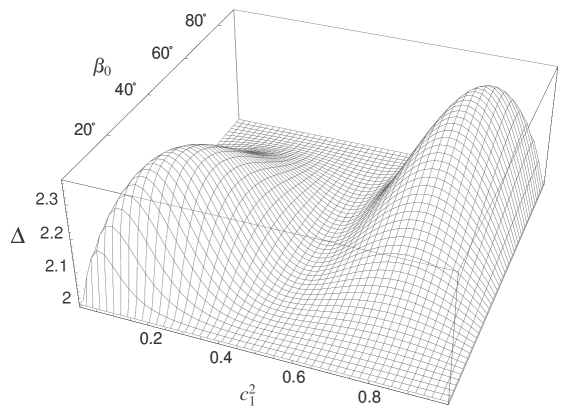
centerlast                  1cm

Fig. 1: Quantum prediction for the parameter $\Delta$ in the case that conditions in Eqs. (8a)-(8c) are satisfied. As explained in the text, the behavior of $\Delta$ is entirely governed by the probability in Eq. (8d), so that $\Delta$ is greater than 2 whenever $P_{\eta}(D_{12}=+1,D_{22}=+1)$ is positive. The surface displayed in the figure fulfills the symmetry property $\Delta(c_{1}^{2},\beta_{0})=\Delta(1-c_{1}^{2},90^{\circ}-\beta_{0})$, so that such a surface stays invariant under a rotation of $n\pi$ ($n=0,\pm 1,\pm 2,\ldots)$ about a vertical axis passing through the point $(c_{1}^{2},\beta_{0})=(0.5,45^{\circ})$.

exception arises because, if $\beta_{0}=n\pi/2$, then by Eqs. (15a)-(15c) we must have necessarily $\beta_{ij}=n_{ij}\pi/2$ for each $i,j=1,2$, and for some $n_{ij}=0,\pm 1,\pm 2,\ldots$ (with $n_{12}=n$). In view of Eq. (6), this in turn implies that perfect correlations would take place between the measurement outcomes for any of the pairs of observables ($D_{1k},D_{2l}$) (see Sec. 2). Further, as may be easily checked, these perfect correlations fulfill $E_{\eta}(D_{11},D_{21})=E_{\eta}(D_{11},D_{22})=E_{\eta}(D_{12},D_{21})=E_{\eta}(D_{12},D_{22})=-1$, and thus $\Delta=2$. It is not difficult to show, on the other hand, that the expression (18) remains invariant under the joint transformations $c_{1}^{2}\rightarrow c_{2}^{2}=1-c_{1}^{2}$ and $\beta_{0}\rightarrow\pm\beta_{0}+m\pi/2$, $m=\pm 1,\pm 3,\ldots$ . In fact, the greatest value of $\Delta$ is attained for both sets of points $(c_{1}^{2},\beta_{0})=(0.177\,\,352,\pm 17.5566^{\circ}+n\pi)$ and $(c_{1}^{2},\beta_{0})=(0.822\,\,648,\pm 72.4434^{\circ}+n\pi)$, where $n=0,\pm 1,\pm 2,\ldots$ . This greatest value is $\Delta_{g}=2.360\,\,679$ or, in closed notation, $2+4\tau^{-5}$, with $\tau$ being the golden mean $\frac{1}{2}(1+\sqrt{5})$. The quantity $\Delta_{g}-2$ corresponds to approximately 43.5% of the maximum violation $2\sqrt{2}-2$ predicted by quantum mechanics of the CHSH inequality.

It is worthwhile to mention that the graph for $\Delta$ in Fig. 1 has quite the same shape as the graphical representation of the probability $P_{\eta}(D_{12}=+1,D_{22}=+1)$ in Eq. (8d) (this latter graph can be found in Ref. 6), the only relevant difference being the respective ranges of variation of the values taken by such functions, namely, $[2,2+4\tau^{-5}]$ for $\Delta$, and $[0,\tau^{-5}]$ for $P_{\eta}(D_{12}=+1,D_{22}=+1)$. Indeed, we have proved with the aid of a computer program that the whole expression (18) is connected with the probability function $P_{\eta}(D_{12}=+1,D_{22}=+1)$ (which is given explicitly by the fourth term on the right-hand side of Eq. (18)) through the simple relation

$$\Delta=2+4P_{\eta}(D_{12}=+1,D_{22}=+1)\,.$$ (19)

In particular this means that the parameter $\Delta$ in Eq. (18) is maximum whenever $P_{\eta}(D_{12}=+1,D_{22}=+1)$ so is. Likewise, $\Delta$ takes its minimum value 2 whenever $P_{\eta}(D_{12}=+1,D_{22}=+1)$ vanishes. This close relationship between $\Delta$ and $P_{\eta}(D_{12}=+1,D_{22}=+1)$ was to be expected since the value of $P_{\eta}(D_{12}=+1,D_{22}=+1)$ can be regarded as a direct measure of the degree of “nonlocality” inherent in the Hardy equations (8a)-(8d).

It will further be noted, incidentally, that Hardy’s argument for nonlocality can equally be cast in the form of a simple inequality involving the four probabilities in Eqs. (8a)-(8d) [17]:

$$P_{\eta}(D_{12}=+1,D_{22}=+1)\leq\!\!\!\!\!\!\!\! P_{\eta}(D_{11}=-1,D_{21}=-1)$$

$$+\!\!\!\!\!\!\!\! P_{\eta}(D_{11}=+1,D_{22}=+1)$$

$$+\!\!\!\!\!\!\!\! P_{\eta}(D_{12}=+1,D_{21}=+1)\,.$$ (20)

Quantum mechanics predicts a maximum violation of inequality (20) for the values $P_{\eta}(D_{11}=-1,D_{21}=-1)=P_{\eta}(D_{11}=+1,D_{22}=+1)=P_{\eta}(D_{12}=+1,D_{21}=+1)=0$, and $P_{\eta}(D_{12}=+1,D_{22}=+1)=\tau^{-5}$. The point to be stressed here is that, for this same set of values, quantum mechanics predicts a violation of the CHSH inequality which is four times bigger than that obtained for the inequality (20). It is therefore concluded that, in order to achieve a more conclusive, clear-cut experimental verification of Hardy’s nonlocality theorem [1], one could try to measure the observable probabilities in Eq. (17), once the conditions $P_{\eta}(D_{11}=-1,D_{21}=-1)=P_{\eta}(D_{11}=+1,D_{22}=+1)=P_{\eta}(D_{12}=+1,D_{21}=+1)=0$, and $P_{\eta}(D_{12}=+1,D_{22}=+1)=\tau^{-5}$ have been established.

Bell inequalities should be satisfied by any realistic theory fulfilling a very broad and general locality condition according to which the real factual situation of a system must be independent of anything that may be done with some other system which is spatially separated from, and not interacting with, the former [8, 20]. When applied to our particular situation, this requirement essentially means that the effect of the choice of the observable $D_{i1}$ or $D_{i2}$ to be measured on particle $i$, $i=1,2$, cannot influence the result obtained with another remote measuring device acting on the other particle. For this class of theories the ensemble (measurable) probability of jointly obtaining the result $D_{1k}=\pm 1$ for particle 1 and the result $D_{2l}=\pm 1$ for particle 2, has the functional form [2, 21, 22]

$$P_{\text{HV}}(D_{1k}=\pm 1,D_{2l}=\pm 1)=\int_{\Lambda}d\lambda\,\rho(\lambda)P\left(D_{1k}=\pm 1\right|\lambda)P\left(D_{2l}=\pm 1\right|\lambda)\,.$$ (21)

In Eq. (21), $\lambda$ is a set of variables (with domain of variation $\Lambda$) representing the complete physical state of each individual pair of particles 1 and 2 emerging from the source, $\rho(\lambda)$ is the (normalized) hidden-variable distribution function for the initial joint state of the particles, and $P(D_{ij}=\pm 1\left|\lambda\right)$ is the probability that an individual particle $i$ in the state $\lambda$ gives the result $\pm 1$ for a measurement of $D_{ij}$. Note that both $\rho(\lambda)$ and $\Lambda$ are independent of the actual setting $j=1$ or $2$ corresponding, respectively, to a measurement of $D_{i1}$ or $D_{i2}$ on particle $i$. As is well known, classical probabilities of the form (21) lead to validity of the inequality $\Delta\leq 2$ (and, generally speaking, to validity of any other Bell-type inequality). This is usually proved by invoking certain algebraic theorems (see, for instance, Ref. 22 for a derivation of Bell’s inequality in the context of actual optical tests of local hidden-variable theories). Since the fulfillment of all the Hardy conditions (8a)-(8d) implies the quantum mechanical violation of the inequality $\Delta\leq 2$ (see Fig. 1), it is concluded that no set of probabilities of the form (21) exists which generally reproduces the quantum prediction (18). The most remarkable exception to this statement is the case where $\left|c_{1}\right|=\left|c_{2}\right|$. For this case quantum mechanics predicts $\Delta=2$, and then, as was discussed in Sec. 3, a rather trivial classical model of the type considered can be constructed which accounts for each of the quantum perfect correlations $E_{\eta}(D_{11},D_{21})=E_{\eta}(D_{11},D_{22})=E_{\eta}(D_{12},D_{21})=E_{\eta}(D_{12},D_{22})=\pm 1$.

5 Concluding remarks

A final comment is in order about the fact that maximally entangled states yield the maximum quantum mechanical violation of Bell’s inequality, while they are unable to exhibit Hardy-type nonlocality. The explanation for this seeming contradiction simply relies on the fact that the rather stringent constraints (11a)-(11d) implied by the Hardy equations (8a)-(8c) in the case of a maximally entangled state, are not at all present in the derivation of Bell’s inequality. Indeed, in the case of Bell’s theorem, all the parameters $\beta_{1k}$, $\beta_{2l}$, $\delta_{1k}$, and $\delta_{2l}$ ($k,l=1,2$) are treated as independent variables which can assume any arbitrary value regardless of the quantum state $\left|\eta\right\rangle$ at issue, so that the Bell inequality will in fact be maximally violated for a suitable choice of $\beta_{ij}$ and $\delta_{ij}$ (provided $\left|c_{1}\right|=\left|c_{2}\right|$). So, consider the case in which $2c_{1}c_{2}\cos\delta_{1k2l}=+1$ for each $k$ and $l$. For this case the quantum prediction for $\Delta$ is given by

$$\Delta=\left|\cos 2(\beta_{11}-\beta_{21})+\cos 2(\beta_{11}-\beta_{22})+\cos 2(\beta_{12}-\beta_{21})-\cos 2(\beta_{12}-\beta_{22})\right|,$$ (22)

which attains the value $\Delta=2\sqrt{2}$ whenever $\beta_{11}-\beta_{21}=-\pi/8$, $\beta_{11}-\beta_{22}=\pi/8$, $\beta_{12}-\beta_{21}=\pi/8$, and $\beta_{12}-\beta_{22}=3\pi/8$. Only if the parameters $\beta_{ij}$ are constrained to obey the relations (11a)-(11d), as demanded by the Hardy equations (8a)-(8c) in the case of maximal entanglement, we have that $\beta_{1k}-\beta_{2l}=m_{1k2l}\pi/2$ for each $k$ and $l$, and for some odd integer $m_{1k2l}$ (for instance, $\beta_{11}-\beta_{21}=-\pi/2$, $\beta_{11}-\beta_{22}=\pi/2$, $\beta_{12}-\beta_{21}=\pi/2$, and $\beta_{12}-\beta_{22}=3\pi/2$), and then $\Delta=2$. Consider now the particular case in which $\left|c_{1}\right|=\left|c_{2}\right|=2^{-1/2}$, $\beta_{11}=\pi/4$, $\beta_{12}=-3\pi/4$, $\beta_{21}=3\pi/4$, and $\beta_{22}=-\pi/4$ (with the parameters $\delta_{1k}$ and $\delta_{2l}$ taking on any arbitrary value). For this case the quantum prediction for $\Delta$ becomes

$$\Delta=\left|\cos(\delta_{11}-\delta_{21})+\cos(\delta_{11}-\delta_{22})+\cos(\delta_{12}-\delta_{21})-\cos(\delta_{12}-\delta_{22})\right|,$$ (23)

which attains the value $2\sqrt{2}$ for $\delta_{11}-\delta_{21}=-\pi/4$, $\delta_{11}-\delta_{22}=\pi/4$, $\delta_{12}-\delta_{21}=\pi/4$, and $\delta_{12}-\delta_{22}=3\pi/4$. However, the fulfillment of the Hardy equations (8a), (8b), and (8c) requires, respectively, that $\delta_{1121}=n_{1121}\pi$, $\delta_{1122}=n_{1122}\pi$, and $\delta_{1221}=n_{1221}\pi$. In particular, the choice $\delta_{1121}=\delta_{1122}=\delta_{1221}=0$ entails that $\delta_{1222}=0$, and therefore, for such values, the quantity $\Delta$ takes again the value 2.

To summarize, we have shown that whenever the Hardy equations (8a)-(8c) are fulfilled for the maximally entangled state then perfect correlations develop between the measurement outcomes $D_{1k}=m$ and $D_{2l}=n$ obtained in any one of the four possible combinations of joint measurements ($D_{1k},D_{2l}$) one might actually perform on both particles. As a result, for such observables $D_{ij}$, the quantity $\Delta$ turns out to be equal to 2, and hence no violations of local realism will arise in those circumstances. This is in contrast with the situation entailed by Bell’s theorem (with inequalities) where no constraints such as Eqs. (8a)-(8c) need be fulfilled, and then all the relevant parameters can be varied freely. On the other hand, for the nonmaximally entangled case, we have generally shown that the fulfillment of conditions (8a)-(8c) necessarily makes the parameter $\Delta$ greater than 2, the greatest value of $\Delta$ predicted by quantum mechanics being as large as $\Delta_{g}=2+4\tau^{-5}$. As was emphasized in Sec. 4, this result could have some relevance from an experimental point of view, since it indicates that experiments based on the inequality $\Delta\leq 2$ (with $\Delta$ given by Eq. (17)) would be more efficient in order to exhibit Hardy’s nonlocality than those based on inequality (20).

Acknowledgments — The author wishes to thank Agustín del Pino for his interest and many useful discussions on the foundations of quantum mechanics. He would also like to thank an anonymous referee for his valuable suggestions which led to an improvement of an earlier version of this paper.

APPENDIX

The demonstration of the lemma is as follows. Here we give only the proof that the vanishing of the probability function (3a) for the case that $\cos\delta_{1k2l}=+1$, is equivalent to the fulfillment of relation (9a), the proof concerning the equivalence of relation (9b) and the vanishing of Eq. (3b) being quite similar. We first show necessity, namely, that the vanishing of the probability in Eq. (3a) implies relation (9a), provided that $\cos\delta_{1k2l}=+1$. So, equating expression (3a) to zero, and putting $\cos\delta_{1k2l}=+1$, we get

$$c_{1}^{2}\cos^{2}\beta_{1k}\cos^{2}\beta_{2l}+c_{2}^{2}\sin^{2}\beta_{1k}\sin^{2}\beta_{2l}$$

$$\,\,=-2c_{1}c_{2}\cos\beta_{1k}\cos\beta_{2l}\sin\beta_{1k}\sin\beta_{2l}\,,$$ (A1)

or, equivalently,

$$(c_{1}/c_{2})^{2}\left[\tan\beta_{1k}\tan\beta_{2l}\right]^{-1}+\tan\beta_{1k}\tan\beta_{2l}=-2(c_{1}/c_{2})\,.$$ (A2)

Now, making the identifications $\tan\beta_{1k}\tan\beta_{2l}\equiv x$ and $c_{1}/c_{2}\equiv a$, Eq. (A2) can be rewritten in the form

$$x^{2}+2ax+a^{2}=0\,,$$ (A3)

or,

$$\left(x+a\right)^{2}=0\,.$$ (A4)

Obviously, Eq. (A4) is satisfied only for $x=-a$, and, therefore, it is concluded that the vanishing of the probability (3a) (with $\cos\delta_{1k2l}=+1$) necessarily entails that $\tan\beta_{1k}\tan\beta_{2l}=-c_{1}/c_{2}$.

The proof of sufficiency, namely, that the fulfillment of relation (9a) implies the vanishing of the probability (3a) when $\cos\delta_{1k2l}=+1$, is quite immediate, and it will not be detailed here.

References

- [1] L. Hardy, Phys. Rev. Lett. 71, 1665 (1993).
- [2] J.F. Clauser, M.A. Horne, A. Shimony, and R.A. Holt, Phys. Rev. Lett. 23, 880 (1969); J.F. Clauser and A. Shimony, Rep. Prog. Phys. 41, 1881 (1978).
- [3] S. Goldstein, Phys. Rev. Lett. 72, 1951 (1994).
- [4] T.F. Jordan, Phys. Rev. A 50, 62 (1994); Am. J. Phys. 62, 874 (1994).
- [5] P.K. Aravind, Am. J. Phys. 64, 1143 (1996).
- [6] J.L. Cereceda, Phys. Rev. A 57, 659 (1998).
- [7] D.M. Greenberger, M.A. Horne, A. Shimony, and A. Zeilinger, Am. J. Phys. 58, 1131 (1990).
- [8] A. Einstein, B. Podolsky, and N. Rosen, Phys. Rev. 47, 777 (1935).
- [9] D. Bohm, Quantum Theory, (Prentice-Hall, Englewood Cliffs, NJ, 1951), p. 614.
- [10] A. Aspect, P. Grangier, and G. Roger, Phys. Rev. Lett. 49, 91 (1982).
- [11] A. Ekert and P.L. Knight, Am. J. Phys. 63, 415 (1995).
- [12] A. Fine, Phys. Rev. Lett. 48, 291 (1982); J. Math. Phys. 23, 1306 (1982).
- [13] A. Peres, Phys. Rev. A 54, 2685 (1996).
- [14] J.S. Bell, Physics (Long Island City, NY) 1, 195 (1964).
- [15] B.S. Tsirelson, Lett. Math. Phys. 4, 93 (1980); L.J. Landau, Phys. Lett. A 120, 54 (1987); M. Hillery and B. Yurke, Quantum Opt. 7, 215 (1995).
- [16] G. Krenn and K. Svozil, Found. Phys. 28 (6), 971 (1998).
- [17] N.D. Mermin, Am. J. Phys. 62, 880 (1994).
- [18] J.R. Torgerson, D. Branning, C.H. Monken, and L. Mandel, Phys. Lett. A 204, 323 (1995).
- [19] D. Boschi, F. De Martini, and G. Di Giuseppe, Phys. Lett. A 228, 208 (1997); Phys. Rev. A 56, 176 (1997); D. Boschi, S. Branca, F. De Martini, and L. Hardy, Phys. Rev. Lett. 79, 2755 (1997).
- [20] A. Einstein, in Albert Einstein: Philosopher-Scientist, edited by P. Schilpp (Open Court, La Salle, Ill., 1949), p. 85.
- [21] J.F. Clauser and M.A. Horne, Phys. Rev. D 10, 526 (1974).
- [22] M. Ardehali, Phys. Rev. A 49, R3143 (1994); Phys. Rev. A 47, 1633 (1993).
- [23] S.M. Barnett and A. Chefles, Los Alamos e-print archive quant-ph/9807090.