Are violations to temporal Bell inequalities there
when somebody looks?

Abstract

The possibility of observing violations of temporal Bell inequalities, originally proposed by Leggett and Garg as a mean of testing the quantum mechanical delocalization of suitably chosen macroscopic bodies, is discussed by taking into account the effect of the measurement process. A general criterion quantifying this possibility is defined and shown not to be fulfilled by the various experimental configurations proposed so far to test inequalities of different forms.

1 Introduction

The validity of quantum mechanics at the macroscopic level is still an open question. Leggett and Garg [1] have challenged this question by proposing laboratory tests aimed at comparing, in a macroscopic domain, the predictions of a set of theories incorporating realism and non-invasivity, two properties not shared by quantum mechanics, versus quantum mechanics itself. The test involved certain inequalities, called temporal Bell inequalities in analogy to the well-known spatial ones [2]. These last have been already experimentally studied [3] to understand the validity of quantum mechanics against local realism at the microscopic level. Temporal Bell inequalities instead, involving correlation probabilities between subsequent measurements of the same observable, hold in realistic theories but are violated under certain conditions by quantum mechanics. The general ingredients required to discuss temporal Bell inequalities, regardless of the concrete scheme used, are three: (a) the possibility to have a coherent, quantum evolution of the state; (b) a dichotomic observable, already discrete or derived by a continuous one; (c) different-time correlation probabilities between subsequent measurements of the dichotomic observable. Leggett and Garg originally proposed use of an rf-SQUID, further analyzed in [4], while more recently other configurations have been discussed, such as a two-level atomic system undergoing optically driven Rabi oscillations [5], and Rydberg atoms interacting with a single quantized mode of a superconducting resonant cavity [6]. The proposal of Leggett and Garg has been criticized [7] focusing mainly on the assumptions made in the macrorealistic approaches.

In this Letter we instead consider the full quantum mechanical predictions for the various proposed experiments. The main point of our analysis is that, as in any quantum mechanical prediction, probability distributions for the outcome of subsequent measurements have to be evaluated and compared to the analogous quantities actually measurable in laboratory. In practice, we will restrict ourselves to the evaluation of average and variance of the observed quantities. While the average value is necessary to define the violation itself, its variance is crucial to establish if the corresponding experimental resolution is sufficient to assign in an unambiguous way the value of the dichotomic observable [8]. We will check if, under the experimental conditions which would lead to a contradiction between quantum and classical predictions for the correlation probabilities, the actual resolution can be sufficient to distinguish the two values of the dichotomic observable – otherwise it would be impossible to state that the quantum mechanical probabilities refer to well–defined observables. This feature was not taken into account in any of the previous papers of other authors on the subject [7], and constitutes the main point of our work. Indeed, we have already addressed this point elsewhere [8, 9] referring to specific physical schemes; the novelty of the present contribution is represented by the generality of our consideration, which apply to all experimental proposals put forward so far.

2 Quantum measurements on bistable systems

We begin by briefly reviewing the conventional analysis of quantum measurements on a generic bistable system undergoing oscillations with period $\tau$ between the two states $|+\rangle$ and $|-\rangle$, according to the time evolution operator $\hat{U}(t_{\rm b},t_{\rm a})$. The effect of a measurement of the dichotomic observable $\hat{X}$ is, as usual, represented through a non-unitary measuring operator

$$\hat{\Pi}_{X}^{\dagger}=\hat{\Pi}_{X}\;,\quad\hat{\Pi}_{X}^{2}=1\!\mbox{l}\;,\quad\hat{\Pi}_{X}|x\rangle=\delta_{Xx}|x\rangle\;,$$ (1)

where $|x\rangle=|\pm\rangle$ and $X$ is one of the two eigenvalues $\pm|X|$. Given some initial preparation $|X_{\rm a}\rangle$ at time $t_{\rm a}$, after measurements performed at times $t_{\rm b}$, $t_{\rm c}$ with results $X_{\rm b}$, $X_{\rm c}$ respectively we get

$$|x(t_{\rm b}^{+})\rangle_{X_{\rm a}X_{\rm b}}=\hat{\Pi}_{X_{\rm b}}\hat{U}(t_{\rm b},t_{\rm a})|X_{\rm a}\rangle\;;\qquad|x(t_{\rm c}^{+})\rangle_{X_{\rm a}X_{\rm b}X_{\rm c}}=\hat{\Pi}_{X_{\rm c}}\hat{U}(t_{\rm c},t_{\rm b})|x(t_{\rm b}^{+})\rangle_{X_{\rm a}X_{\rm b}}\;.$$ (2)

The corresponding correlation probabilities are

$$p^{\rm ab}_{X_{\rm a}X_{\rm b}}=||x(t_{\rm b}^{+})||^{2}_{X_{\rm a}X_{\rm b}}\;;\qquad p^{\rm bc}_{X_{\rm a}X_{\rm b}X_{\rm c}}=||x(t_{\rm c}^{+})||^{2}_{X_{\rm a}X_{\rm b}X_{\rm c}}\;,$$ (3)

and their variances, whose square roots are called effective uncertainties, are

$$\left(\Delta X^{\rm ab}_{\rm eff}\right)^{2}={\sum_{x}\left(X_{\rm b}-x\right)^{2}p^{\rm ab}_{X_{\rm a}x}}\;;\qquad\left(\Delta X^{\rm bc}_{\rm eff}\right)^{2}={\sum_{x}\left(X_{\rm c}-x\right)^{2}p^{\rm bc}_{X_{\rm a}X_{\rm b}x}}\;.$$ (4)

Their value is dictated by the laws of quantum mechanics, regardless of the size of the ensemble over which measurements are performed. From the definition Eq. (4) it follows that $0\leq\Delta X_{\rm eff}\leq 2|X|$ at any times. On the other hand, a resolution large enough is required in order to assign to the dichotomic observable a non-zero value without ambiguity. In other words, one has to take as non-ambiguous only measurements for which a condition $\Delta X_{\rm eff}\leq\xi$ is satisfied, the value of the threshold effective uncertainty $\xi$ defining the resolution criterion. A null value of $\xi$ means that only infinite-resolution measurements are taken as non-ambiguous; when $\xi=2|X|$ no discrimination is made between measurements with or without a resolution power sufficient to distinguish the two states $|+\rangle$ and $|-\rangle$. Any of the criteria commonly used in resolution studies [10] can be related to a value of the threshold between these two extremes. For example, the well-known half-width criterion corresponds to $\xi=\xi_{1/2}\equiv(2\ln 2)^{-1/2}|X|$: two probabilities distribution centered at $\pm|X|$ can be resolved if and only if their variance satisfies $\Delta X<\xi_{1/2}$. A less stringent criterion would be for instance to require $\Delta X<|X|$.

3 Temporal Bell inequalities

Temporal Bell inequalities are formally derived by assuming the existence of $n$-times correlation probabilities $p^{t_{1}\cdots t_{n}}_{X_{1}\cdots X_{n}}$ satisfying positive definiteness and completeness, as well as the non-invasive measurability at any intermediate time [1]. Under these conditions, for instance,

$$p^{\rm ac}_{+-}=p^{\rm abc}_{+--}+p^{\rm abc}_{++-}\leq p^{\rm abc}_{+--}+p^{\rm abc}_{+-+}+p^{\rm abc}_{++-}+p^{\rm abc}_{-+-}=p^{\rm ab}_{+-}+p^{\rm bc}_{+-}$$ (5)

which involves measurements performed at the subsequent times $t_{\rm b}$ and $t_{\rm c}$ on a system prepared in state $|+\rangle$ at the initial time $t_{\rm a}$. More in general three types of inequalities, analogous to (5), can be derived:

$$\Delta P_{\rm I}(t_{\rm ab},t_{\rm bc}) \equiv p^{\rm ac}_{X_{\rm a},X_{\rm c}}-p^{\rm ab}_{X_{\rm a},X_{\rm b}}-p^{\rm bc}_{-X_{\rm b},X_{\rm c}}\leq 0\;;$$

$$\Delta P_{\rm II}(t_{\rm ab},t_{\rm bc}) \equiv p^{\rm ab}_{X_{\rm a},X_{\rm b}}-p^{\rm ac}_{X_{\rm a},X_{\rm c}}-p^{\rm bc}_{X_{\rm b},-X_{\rm c}}\leq 0\;;$$ (6)

$$\Delta P_{\rm III}(t_{\rm ab},t_{\rm bc}) \equiv p^{\rm bc}_{X_{\rm b},X_{\rm c}}-p^{\rm ab}_{X_{\rm a},X_{\rm b}}-p^{\rm ac}_{-X_{\rm a},X_{\rm c}}\leq 0\;.$$

While inequalities of type III are ruled out by the experimental requirement that the system is prepared in a definite state at time $t_{\rm a}$, the other two types are in principle well suitable for experimental test. In fact, as originally observed in [1], each one of them is violated for some subset of measurement times $t_{\rm ab}\equiv t_{\rm b}-t_{\rm a}$, $t_{\rm bc}\equiv t_{\rm c}-t_{\rm b}$. On the other hand, the distinguishability criterion is fulfilled for another subset of $(t_{\rm ab},t_{\rm bc})$ depending upon the chosen threshold effective uncertainty $\xi$. It is therefore useful to introduce an overlap integral expressing the average probability difference $\Delta P_{\alpha}$ (where $\alpha={\rm I},{\rm II},{\rm III}$) integrated over all the time intervals for which both temporal Bell inequalities are violated by quantum mechanical predictions and distinguishability is assured by $\Delta X_{\rm eff}\leq\xi$:

$${\cal O}_{\alpha}(\xi)\equiv\frac{1}{\tau^{2}}\int_{\cap}\Delta P_{\alpha}\,{\rm d}t_{\rm ab}\,{\rm d}t_{\rm bc}$$ (7)

where the subscript $\cap$ means that the integration is restricted to the values of $(t_{\rm ab},t_{\rm bc})$ for which $\Delta P_{\alpha}>0$ and $\Delta X_{\rm eff}\leq\xi$ for all measurements in $\Delta P_{\alpha}$. The meaning of the overlap integral Eq. (7) is the following: given a threshold effective uncertainty $\xi$, it provides a measure of whether the violation of a certain temporal Bell inequality is compatible with the discrimination between the two values of the dichotomic observable, according to the criterion defined by $\xi$. From Eq. (7), it follows that ${\cal O}_{\alpha}(\xi)$ is continuous and monotonically increasing with $\xi$. Based on the considerations below Eq. (4), we expect also ${\cal O}_{\alpha}(\xi\to 0)=0$, ${\cal O}_{\alpha}(\xi\to 2|X|)=\tau^{-2}\int_{0}^{\tau}{\rm d}t_{\rm ab}\int_{0}^{\tau}{\rm d}t_{\rm bc}\Delta P_{\alpha}>0$. Therefore the overlap integral will be nonzero only for $\xi$ large enough. We thus define

$$\xi_{\alpha}\equiv\min\{\xi:{\cal O}_{\alpha}(\xi^{\prime})>0,\xi^{\prime}>\xi\}=\max\{\xi:{\cal O}_{\alpha}(\xi^{\prime})<0,\xi^{\prime}<\xi\}.$$ (8)

This has to be compared with the $\xi_{1/2}$ defined above, in order to find out if violation of the inequalities Eq. (6) and discrimination of the two values of $X$ can be obtained in the same experiment. As a tool for our analysis we first discuss a toy model exhibiting all the relevant features intrinsic to the temporal Bell inequalities, moving later to the actual Hamiltonian of a rf-SQUID system as proposed in [4]. We do not take into account finite temperature or imperfect efficiency effects, irrelevant to the arguments we plan to discuss since they can only diminish the chance to observe the predicted violations (see for instance the discussion in [6]).

4 Spin-1/2 particle case

Let us consider a spin-1/2 particle precessing in a uniform magnetic field. Its Hamiltonian is $\hat{H}=-\vec{\sigma}\cdot\vec{B}$ with $\vec{\sigma}=(\sigma_{x},\sigma_{y},\sigma_{z})$ the Pauli matrices and $\vec{B}=(B,0,0)$. The temporal evolution of the state vector is ruled by the operator

$$\hat{U}(t_{\rm b},t_{\rm a})=\exp\left[-\frac{i}{\hbar}B\sigma_{x}(t_{\rm b}-t_{\rm a})\right]\;.$$ (9)

A measurement of the third component of the spin is represented by the projector

$$\hat{\Pi}_{\Sigma}={{1+2\Sigma\sigma_{z}}\over 2}\;,\qquad\Sigma=\pm\frac{1}{2}\;.$$ (10)

The correlation probabilities appearing in (5) are then:

$$p^{\rm ab}_{+-}=\sin^{2}\Omega t_{\rm ab}\;;\qquad p^{\rm ac}_{+-}=\sin^{2}\Omega(t_{\rm ab}+t_{\rm bc})\;;\qquad p^{\rm bc}_{+-}=\cos^{2}\Omega t_{\rm ab}\sin^{2}\Omega t_{\rm bc}\;.$$ (11)

where the angular frequency $\Omega\equiv B/\hbar$ has been introduced, whence the oscillation period $\tau_{\sigma}=2\pi/\Omega=2\pi\hbar/B$. The effective uncertainties are then calculated according to (4). As already pointed out in [9], this discussion applies to the proposals [5] and [6], dealing with the two-level dynamics of atomic systems.

5 SQUID case

In the rf-SQUID case instead the monitored observable is the magnetic flux $\Phi$ threading the ring, a continuous observable. Its sign is a dichotomic variable which is directly measurable in a quantum coherence experimental setup [11]; the corresponding projector is

$$\hat{\Pi}_{\Phi}=\Theta(\Phi\hat{\varphi})\;,\qquad\Phi=\pm 1\;.$$ (12)

The effective Hamiltonian describing the system is [12]

$$\hat{H}=-{\hbar^{2}\over 2C}{{\rm d}^{2}\over{\rm d}\varphi^{2}}+{(\varphi-\Phi^{\rm ext})^{2}\over 2L}-{I_{\rm c}\Phi_{0}\over 2\pi}\cos\left(2\pi{\varphi\over\Phi_{0}}\right)\;,$$ (13)

where $C$ is the weak link capacitance (which plays the role of an effective mass), $L$ the ring inductance, $I_{\rm c}$ the critical current of the junction, $\Phi^{\rm ext}$ is the external magnetic flux threading the ring and the flux quantum $\Phi_{0}=\hbar/2e\approx 2.07\cdot 10^{-15}$ Wb. A bistable regime is obtained if the condition $1<2\pi LI_{\rm c}/\Phi_{0}<5\pi/2$ is fulfilled. In this case, by introducing the adimensional variable $\phi=(\varphi-\Phi^{\rm ext})/\Phi_{0}$ and by fixing the value of the external flux at $\Phi^{\rm ext}/\Phi_{0}=(n+1/2)$, $n\in$ Z the potential can be approximated – up to a constant – by the quartic double-well form

$$V(\phi)=\frac{\pi^{3}}{3}I_{\rm c}\Phi_{0}(\phi-\phi_{0})^{2}(\phi+\phi_{0})^{2}\;,$$ (14)

where the two minima $\pm\phi_{0}$ are the solutions of the equation $\sin(2\pi\phi)/\phi=\Phi_{0}/LI_{\rm c}$ and are separated by a barrier of height $\Delta V=(\pi^{3}/3)I_{\rm c}\Phi_{0}\phi_{0}^{4}$. Correspondingly, the ground state has two peaks localized around $\pm\phi_{0}$, each of width $\sigma_{0}$ determined by the approximate relationship $C\omega_{0}^{2}\sigma_{0}^{2}/2\simeq\hbar\omega_{0}/4$ where $\omega_{0}$ is the plasma frequency, i.e. the angular frequency of the small oscillations around $\pm\phi_{0}$. A flux wavepacket localized at $\pm\phi_{0}$ is a superposition of the ground and first excited state and has width $\sigma_{0}$. If no measurement is performed, such a state will undergo coherent tunneling oscillations between the two wells with period $\tau_{\phi}\equiv 2\pi\hbar/\Delta E_{0}$, where $\Delta E_{0}$ is the splitting between the lowest two energy eigenvalues. This last decreases exponentially with increasing barrier height, whereas the tunneling frequency should be at least of the order of magnitude of 1 MHz – otherwise the coherent oscillations would be damped by the interaction with the environment. On the other hand, in order to treat the system as a two-level one [1], the probability for finding the system in the barrier region around $\phi=0$ should be negligible; in other words, it should be $\sigma_{0}^{2}\ll\phi_{0}^{2}$, which in turn could be achieved with a high enough barrier. It is possible to choose the parameters in (13) in order to satisfy both these requirements: indeed, with $L=150pH$, $C=0.15pF$ and $I_{\rm c}=2.5\mu A$ (very close to the values used in [4]) it is $\tau_{\phi}^{-1}\approx 5.94\;\mbox{MHz}$ and $\sigma_{0}^{2}/\phi_{0}^{2}\approx 0.08$.

6 Results and discussion

In fig. 1 the overlap integral defined in Eq. (7) is plotted as function of $\xi$ for all the inequalities of the form (5).

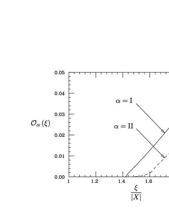
Fig. 1.–: Overlap integral for inequalities of type I and II, as function of the effective uncertainty threshold $\xi$ (in units of $|X|$), with any combinations of measurement results $X_{a}$, $X_{b}$ and $X_{c}$.

The result depicted here is valid both for the spin toy-model and for the actual SQUID Hamiltonian (with the parameters quoted above), which lead to identical predictions because, as the tunneling oscillations dominate the dynamics, the two-level approximation is appropriate to describe the flux correlation probabilities in the rf-SQUID. No dependence on the actual values of $X_{\rm a}$, $X_{\rm b}$ and $X_{\rm c}$ is seen, but only on the type of inequality. The type I turns out to be more favourable for the observation of violations. Nevertheless, as it can be seen from the Figure, in both cases $\xi_{\alpha}>1.4|X|$, which is greater than any reasonable resolution threshold. This is the main result of this Letter showing that, even in the most favourable situation, it is impossible to observe violations to temporal Bell inequalities predicted by quantum mechanics maintaining at the same time the resolution high enough to distinguish the two values of the dichotomic observable.

The correlation probabilities (3) are obtained by means of the standard rules of quantum mechanics from the corresponding interfering amplitudes. The violation of the inequality (5) however may be understood by noticing that it necessarily implies that at least one of the three time correlation probabilities $p_{ijk}^{\rm abc}$ becomes negative, namely becomes a Wigner function (pseudoprobability). This means, according to Feynman [13], that “the assumed condition of preparation or verification are experimentally unattainable” as a consequence of the uncertainty principle which forbids the existence of joint probabilities for incompatible variables. For instance, in our case from (5) follows that, when $X_{\rm a}=-X_{\rm b}=-X_{\rm c}=|X|$ in (6), $\Delta P_{\rm I}=-p_{+-+}^{\rm abc}$: therefore in the region where the temporal Bell inequality is violated, at least one of the joint pseudoprobabilities at three different times is negative. This result holds in general – and is no surprise. One should remember in fact that Wigner’s proof [14] of validity of spatial Bell inequalities is based on the assumption, analogous to that made before Eq. (5), of non-negative joint probabilities for the spin components along different directions. Their violation should be ascribed, therefore, to the uncertainty principle which prevents the existence of these non-negative joint probabilities. This consequence of the uncertainty principle is independently confirmed by a recent result [15] according to which the violation of spatial Bell inequalities is directly connected to the appearance of negative conditional entropies, a feature which is classically forbidden.

On the other hand, and this is the difference between spatial and temporal Bell inequalities, it is the uncertainty principle itself which introduces in our case a constraint on the ability to resolve the two states in a second measurement at a later time on the same particle. (Such a constraint does not exist when the two measurements are performed at the same time on two different particles located in different space points). This second constraint arises from the fact that, as discussed in detail in [8], a quantum measurement of a given observable induces a perturbation in the evolution of its canonical conjugate, and this in turn produces an uncertainty on the outcome of a measurement of the same variable at a later time. This is crucial because, as we mentioned at the beginning of this paper, repeating measurements on the same observable is precisely what discriminates temporal Bell inequalities from the spatial version, where two different systems are observed only once. These two constraints, both arising from the uncertainty principle, are, as we have seen, conflicting, because the region in which the violations arise and the region in which the resolution is high enough to resolve between the two states do not overlap.

These general considerations should affect other situations in which a macroscopic quantum system is repeatedly measured, for instance an atomic Bose-Einstein condensate in which the Josephson dynamics is studied. At the very core of quantum mechanics, the uncertainty principle has two competing consequences when applied to a single macroscopic system repeatedly monitored, the violation of classical probability laws for predictions on a dichotomic observable and the limitations on the resolution of the observable itself, and it seems impossible to experimentally unravel these two features without conflict.

***

We thank C. Cosmelli and C. Kuklewicz for useful discussions, and L. Chiatti for comparison of codes simulating the behaviour of the rf-SQUID. One of us (T. C.) thanks the Institute of Nuclear Theory at the University of Washington and the Department of Physics at the University of Trento (in particular M. Traini and S. Stringari) for their hospitality, the Department of Energy and the ECT* and INFN in Trento for partial support during the completion of this work, and A. J. Leggett and A. Garg for stimulating discussions.

References

- [1] Leggett A.J. and Garg A., Phys. Rev. Lett., 54 (1985) 857.
- [2] Bell J.S., Physics, 1 (1964) 195; Speakable and unspeakable in quantum mechanics: collected papers in quantum mechanics, (Cambridge University Press) 1987, in particular pp. 14-21.
- [3] Aspect A. et al., Phys. Rev. Lett., 47 (1981) 460.
- [4] Tesche C.D., in Proc. NY Conf. on Quantum Measurement Theory, (New York Academy of Sciences, New York) 1986, pp. 36; Phys. Rev. Lett., 64 (1990) 2358.
- [5] Paz J.P. and G. Mahler, Phys. Rev. Lett., 71 (1993) 3235.
- [6] Huelga S.F., Marshall T.W. and Santos E., Phys. Rev., A52 (1995) R2497; Phys. Rev., A54 (1996) 1798.
- [7] Ballentine L.E., Phys. Rev. Lett., 59 (1987) 1493; see also the reply of Leggett A.J. and Garg A., Phys. Rev. Lett., 59 (1987) 1621; Peres A., Phys. Rev. Lett., 61 (1988) 2019; see also the reply of Leggett A.J. and Garg A., Phys. Rev. Lett., 63 (1989) 2159; Foster S. and A. Elby A., Found. Phys., 21 (1991) 773; Hardy L., Home D., Squires E.J. and Whitaker M.A.B., Phys. Rev., A45 (1992) 4267; Benatti F., Ghirardi G.C. and Grassi R., Found. Phys. Lett., 7 (1994) 105; Chiatti L., Cini M. and Serva M., Nuovo Cimento, B110 (1995) 585.
- [8] Onofrio R. and Calarco T., Phys. Lett., A208 (1995) 40.
- [9] Calarco T. and Onofrio R., Appl. Phys., B64 (1997) 141.
- [10] Condon E.U. and Odishaw H., Handbook of Physics, (McGraw-Hill Book Company, NewYork) 1967.
- [11] Castellano M.G. et al., J. Appl. Phys., 80 (1996) 2922.
- [12] Barone A. and Paternò G., Physics and Applications of the Josephson effect, (John Wiley and Sons Publishing, New York) 1982.
- [13] Feynman R.P., in Quantum Implications: essays in honours of David Bohm, edited by Hiley B.J. and Peat F.D., (Routledge & Kegan, London) 1987, pp. 235; see also the discussion in Scully M.O., Walther H. and Schleich W., Phys. Rev., A49 (1994) 1562.
- [14] Wigner E., Am. Journ. Phys., 38 (1970) 1005.
- [15] Cerf N.J. and Adami C., Phys. Rev., A55 (1997) 3371.