Carmichael Numbers on a Quantum Computer

Abstract

We present a quantum probabilistic algorithm which tests with a polynomial computational complexity whether a given composite number is of the Carmichael type. We also suggest a quantum algorithm which could verify a conjecture by Pomerance, Selfridge and Wagstaff concerning the asymptotic distribution of Carmichael numbers smaller than a given integer.

]

I Introduction

In the last few years the area of quantum computation has gained much momentum (for a review see, e.g., ref. [2]). The power of quantum computers is mainly due to the possibility of working with a superposition of $|0>$ and $|1>$ qubits with coefficients being complex numbers $\alpha$ and $\beta$, i.e. with states $|\psi>=\alpha|0>+\beta|1>$, providing an enormous number of parallel computations by the generation of a superposed state of a large number of terms. Quantum computers can do unitary transformations and (final) measurements inducing an instantaneous state reduction to $|0>$ or $|1>$ with the probability $|\alpha|^{2}$ or $|\beta|^{2}$, respectively [1]. Two of the most important achievements so far have been the discoveries of the quantum algorithms for factoring integers [3] and for the search of unstructured databases [4], which achieve, respectively, an exponential and a square root speed up compared to their classical analogues. Another interesting algorithm exploiting the above mentioned ones in conjunction is that counting the cardinality $t$ of a given set of elements present in a flat superposition of states [5].

In a recent work [6], we showed how an extended use of this counting algorithm can be further exploited to construct unitary and fully reversible operators emulating at the quantum level a set of classical probabilistic algorithms. Such classical probabilistic algorithms are characterized by the use of random numbers during the computation, and they give the correct answer with a certain probability of success, which can be usually made exponentially close to one by repetition. The quantum randomized algorithms described in ref. [6] also naturally select the ’correct’ states with a probability and an accuracy which can be made exponentially close to one in the end of the computation, and since the final measuring process is only an option which may not be used, they can be included as partial subroutines for further computations in larger and more complex quantum networks. As explicit examples, we showed how one can design polynomial time algorithms for studying some problems in number theory, such as the test of the primality of an integer, of the ’prime number theorem’ and of a certain conjecture about the asymptotic number of representations of an even integer as a sum of two primes.

In this paper we will use the methods of ref. [6] to build a polynomial time quantum algorithm which checks whether a composite number $k$ is of Carmichael type. We start in section II by recalling the main definitions and properties of Carmichael numbers. In section III we describe the quantum algorithm for the test of Carmichael numbers. Section IV is devoted to the description of a quantum algorithm which counts the number of Carmichaels smaller than a given integer. Finally, we conclude in section V with some discussion on the results obtained.

II Carmichael numbers

Carmichael numbers are quite famous among specialists in number theory, as they are quite rare and very hard to test. They are defined as composite numbers $k$ such that [7, 8]

$$a^{k-1}\equiv 1~{}~{}\bmod~{}k$$ (1)

for every base $1<a<k$, $a$ and $k$ being relative coprimes, or $GCD(a,k)=1$. For later convenience, we also introduce the function $G_{k}(a)\equiv\Theta[GCD(a,k)]$, where $\Theta[1]=1$ and $\Theta=0$ otherwise. In particular, it can be shown that an integer $k$ is a Carmichael number if and only if $k$ is composite and the maximum of the orders of $a$ mod $k$, for every $1\leq a<k$ coprime to $k$, divides $k-1$. It then follows that every Carmichael number is odd and the product of three or more distinct prime numbers (the smallest Carmichael number is $561=3\times 11\times 17$). Recently, it has also been proven that there are infinitely many Carmichael numbers [9]. On a classical computer, it is hard to test whether a composite number $k$ is Carmichael, as it requires $O[k/\log\log k]$ evaluations of $a^{k-1}~{}\bmod~{}k$.

In principle, there is a quite straightforward method to check whether a composite number $k$ is of the Carmichael type, provided a complete factorization of $k$ itself is known. The algorithm would use the fact that the number of bases $1<a<k$ coprime to $k$ and which satisfy eq. (1), i.e. for which $k$ is a pseudoprime, can be written as $F(k)=\prod_{p_{i}}~{}GCD(p_{i}-1,k-1)$, where the $p_{i}$’s are the prime factors of $k$, i.e. $k=\prod p_{i}^{l}$ [10, 11]. If $k$ is Carmichael, using Lagrange theorem one can easily show that $F(k)$ must be equal to the Euler function $\phi(k)$, which represents the number of integers smaller than $k$ and coprime with $k$. Since, given $k=\prod p_{i}^{l}$, the Euler function is also known and equal to $\phi(k)=k\prod_{p_{i}}(1-1/p_{i})$ [7], the algorithm would only require the complete factorization of $k$ and the evaluation of $F(k)$ and $\phi(k)$. Unfortunately, since the simple use of Shor’s quantum algorithm by itself does not look as an efficient tool for the full factorization of a composite integer (as it would require intermediate tests of primality, see, e.g., our comments in ref. [6]), this method does not look much promising at present.

Instead, in this paper we will describe a quantum algorithm which directly tests whether a composite number is of Carmichael type without the need of knowing a priori a complete factorization of $k$, but by counting how many bases $a$ satisfy condition (1). The power of the algorithm relies on a particular property of the function $F(k)$, i.e. that for an arbitrary composite integer $k$, $F$ divides $\phi$, or $F(k)=\phi(k)/m$, with $m=1,2,...$ (see, e.g., ref. [12]). In particular, if $k$ is Carmichael we have $m=1$, while if $k$ is not Carmichael we have $m\geq 2$. In other words, if $k$ is Carmichael, then there are no bases $a$ which do not satisfy condition (1), while if $k$ is not Carmichael, then at least half of the bases $a$ satisfy this condition. It is mainly the existence of such a gap which allow us to design an efficient quantum probabilistic algorithm for the certification of Carmichael numbers.

III Is $k$ Carmichael ?

The main idea underlying our quantum computation is the repeated use of the counting algorithm COUNT originally introduced by Brassard et al. [5]. The algorithm COUNT makes an essential use of Grover’s unitary operation $G$ for extracting some elements from a flat superposition of quantum states, and Shor’s Fourier operation $F$ for extracting the periodicity of a quantum state. Grover’s unitary transformation is given by $G=-WS_{0}WS_{1}$, where the Walsh-Hadamard transform $W$ is defined as

$$W|a>\equiv{1\over\sqrt{k}}\sum_{b=0}^{k-1}(-1)^{a\cdot b}|b>$$ (2)

(with $a\cdot b$ being the qubitwise product of $a$ and $b$), $S_{0}\equiv I-2|0><0|$ and $S_{1}\equiv I-2\sum_{w}|w><w|$, where $|w>$ are the searched states. Shor’s operation is, instead, given by the Fourier transform

$$F|a>\equiv{1\over\sqrt{k}}\sum_{b=0}^{k-1}e^{2i\pi ab/k}|b>.$$ (3)

The COUNT algorithm can be summarized by the following sequence of operations:

COUNT:

1) $(W|0>)(W|0>)=\sum_{m=0}^{P-1}|m>\sum_{a=0}^{k-1}|a>$

2) $\rightarrow(F\otimes I)[\sum_{m=0}^{P-1}|m>G^{m}(\sum_{a=0}^{k-1}|a>)]$

3) $\rightarrow\mbox{measure}~{}~{}|m>$.

Since the amplitude of the set of states $|w>$ after $m$ iterations of $G$ is a periodic function of $m$, the estimate of such a period by Fourier analysis and the measurement of the ancilla qubit $|m>$ will give information on the size $t$ of this set, on which the period itself depends. The parameter $P$ determines both the precision of the estimate $t$ and the computational complexity of the COUNT algorithm (which requires $P$ iterations of $G$).

Our quantum algorithm uses COUNT for estimating the number $t_{k}\equiv\phi(k)-F(k)$ of bases for which a given composite $k$ is not pseudoprime (i.e. the number of bases comprimes to $k$ which do not satisfy condition (1)), and of $R$ ancilla qubits $|m_{i}>$ which will be finally measured. At first, we have to select the composite number $k$, which can be done, e.g., by use of the quantum analogue of Rabin’s randomized primality test [13] as described in ref. [6], and which will take only $poly(\log k)$ steps. We can then proceed with the main core of the quantum Carmichael test algorithm, by starting with the state

$$|\psi_{0}>\equiv|0>_{1}....|0>_{R}|0>|0>,$$ (4)

act on each of the first $R+1$ qubits with a Walsh-Hadamard transform $W$, producing, respectively, the flat superpositions $\sum_{m_{i}=0}^{P-1}|m_{i}>/\sqrt{P}$, for $i=1,...R$, and $\sum_{a=0}^{k}|a>/\sqrt{k}$, then perform a $CTRL-NOT$ operation on the last qubit (i.e., flipping the value of this qubit) subject to the condition that the state $|a>$ is coprime with $k$, and finally act on the $|a>$ qubits with an $|m_{1}>....|m_{R}>$-’controlled’ Grover operation $G^{m}$ selecting the bases $|a>$ for which $k$ is not a pseudoprime from those for which it is a pseudoprime. We thus obtain the state

$$|\psi_{1}> \equiv {\sum_{m_{1}=0}^{P-1}|m_{1}>\over\sqrt{P}}....{\sum_{m_{R}=0}^{P-1}|m_{R}>\over\sqrt{P}}$$ (5)

$$\times {G^{\sum_{i=1}^{R}m_{i}}\over\sqrt{k}}[\sum_{G_{k}=1}|a>|1>+\sum_{G_{k}=0}|a>|0>],$$ (6)

where for $G$ we use $S_{1}\equiv I-2\sum_{Z_{k}(a)=0}|a><a|$, with the function $Z_{k}(a)$ defined as $Z_{k}(a)=0$ when condition (1) is not satisfied, and $Z_{k}(a)=1$ if condition (1) is satisfied. In the following we will also assume that $P\simeq O[poly(\log k)]$, so that the steps required to compute the repeated Grover operations $G^{m_{1}+....+m_{R}}$ is polynomial in $\log k$.

We then define the quantities

$$\sin\theta_{k}\equiv\sqrt{t_{k}\over k}$$ (7)

and

$$k_{m_{1}....m_{R}} \equiv \sin[2(m_{1}+....+m_{R})+1]\theta_{k}$$ (8)

$$l_{m_{1}....m_{R}} \equiv \cos[2(m_{1}+....+m_{R})+1]\theta_{k},$$ (9)

where $t_{k}$ is the number of bases $a$ for which $Z_{k}(a)=0$, and the states

$$|B_{1}^{k}> \equiv {1\over\sqrt{t_{k}}}\sum_{Z_{k}(a)=0}|a>$$ (10)

$$|B_{2}^{k}> \equiv {1\over\sqrt{\phi(k)-t_{k}}}\sum_{Z_{k}(a)=1}|a>.$$ (11)

Next we apply Shor’s Fourier transform on each of the first $R$ ancilla qubits in order to extract the periodicity $\theta_{k}$ which is hidden in the amplitudes $k_{m_{1}....m_{R}}$ and $l_{m_{1}....m_{R}}$, i.e. we transform $|\psi_{1}>$ into

$$|\psi_{2}> \equiv {\sum_{m_{1},l_{1}=0}^{P-1}e^{2i\pi l_{1}m_{1}/P}|l_{1}>\over P}....$$ (12)

$$\times {\sum_{m_{R},l_{R}=0}^{P-1}e^{2i\pi l_{R}m_{R}/P}|l_{R}>\over P}$$ (13)

$$\times [(k_{m_{1}....m_{R}}|B_{1}^{k}>+l_{m_{1}....m_{R}}|B_{2}^{k}>)|1>$$ (14)

$$+ |Rest>|0>],$$ (15)

where the state $|Rest>$ is the result of the operation $G^{m}$ acting on the bases $|a>$ which are not coprime with $k$.

Finally, we perform a measurement of the last qubit. If we get $|0>$, we start again the whole algorithm from eq. (4). If, instead, we obtain $|1>$, we can proceed since eq. (15) is reduced to the state (which contains only bases for which $G_{k}(a)=1$)

$$|\psi_{3}> \equiv {1\over 2}\sum_{l_{1},...l_{R}=0}^{P-1}|l_{1}>....|l_{R}>e^{-i\pi(l_{1}+....+l_{R})P}$$ (16)

$$\times \biggl{[}e^{i\pi f_{k}^{(R)}}\prod_{i=1}^{R}s_{l_{i}+}^{(P)}(-i|B_{1}^{k}>+|B_{2}^{k}>)$$ (17)

$$+ e^{-i\pi f_{k}^{(R)}}\prod_{i=1}^{R}s_{l_{i}-}^{(P)}(i|B_{1}^{k}>+|B_{2}^{k}>)\biggr{]},$$ (18)

where we have introduced the following quantities,

$$f_{k} \equiv {P\theta_{k}\over\pi}~{}~{}~{}~{};~{}~{}~{}~{}0\leq f_{k}\leq{P\over 2}$$ (19)

$$f_{k}^{(R)} \equiv f_{k}\left[R+{(1-R)\over P}\right]$$ (20)

and

$$s_{l_{i}\pm}^{(P)}\equiv{\sin\pi(l_{i}\pm f_{k})\over P\sin[\pi(l_{i}\pm f_{k})/P]}.$$ (21)

It is easy to see that the probability of measuring the last qubit in eq. (15) in the state $|1>$ is given by $P_{|1>}=\phi(k)/k$, which means that (using the asymptotic behaviour $\phi(k)\simeq k/\log\log k$) we require an average number $T_{av}\simeq(P_{|1>})^{-1}\simeq O[\log\log k]$ of steps to obtain eq. (18).

Now, with eq. (18) at hand, we can count the bases coprime with $k$ for which $k$ is not a pseudoprime. There are then two possibilities: either $k\equiv k_{C}$ is Carmichael, in which case $t_{k_{C}}=0$ and therefore $\theta_{k_{C}}=f_{k_{C}}=0$; or $k\equiv k_{NC}$ is not Carmichael, for which $t_{k_{NC}}\geq{k_{NC}}/2$ and $\theta_{k_{NC}}\geq\pi/4$, implying that $P/4\leq f_{k_{NC}}\leq P/2$. Looking at eq. (18), we can see that, in the case when $k$ is Carmichael, $G$ effectively acts as an identity operator, so that $|\psi_{3}>$ simplifies to

$$|\psi_{3}>\rightarrow|0>_{1}....|0>_{R}|B_{2}^{k}>~{}~{}~{}~{};~{}~{}~{}~{}\mbox{when $k=k_{C}$}.$$ (22)

On the other hand, when $k$ is not Carmichael, almost all of the ancilla qubits in $|\psi_{3}>$ will be in a state different from $|0>_{1}....|0>_{R}$. In fact, the probability of finally measuring $|0>_{1}....|0>_{R}$ when $k$ is not Carmichael is given by

$$P(|0>_{1}....|0>_{R})\biggr{|}_{k_{NC}} = \left({\sin\pi f_{k}\over P\sin{\pi f_{k}\over P}}\right)^{2R}\biggr{|}_{k_{NC}}$$ (23)

$$\equiv (\alpha_{k})^{2R}\biggr{|}_{k_{NC}}\leq\left({\sqrt{2}\over P}\right)^{2R},$$ (24)

since we have that $f_{k_{NC}}\geq P/4$.

The quantum algorithm is probabilistic since, if in the final measurement process of the $R$ ancilla qubits we obtain a state with at least one of the qubits different from $|0>$, we can declare with certainty that the number $k$ is not Carmichael; on the other hand, if all the ancilla qubits are in the state $|0>$, we can claim with an error probability smaller than $O[P^{-2R}]$ that the number $k$ is Carmichael.

One important feature of the quantum algorithm is that clearly, if the intermediate and final measurement steps are omitted, it is unitary and fully reversible, and as such it can be used as a subroutine unitary transform inside a larger and more complicated algorithm (see next section). Another crucial feature is the existence of a gap between the cardinalities (essentially $F(k)$) of the domain of the test function $Z_{k}(a)$ when $k$ is Carmichael and when it is not.

Finally, the computational complexity of the quantum algorithm can be written as $S_{P}\simeq O[kRPS_{G}/\phi(k)]$, with the number of steps required for $G$ given (using $P\simeq O[poly(\log k)]$) by $S_{G}\simeq O[poly(\log k)]$, so that we get $S_{P}\simeq O[R~{}poly(\log k)(\log\log k)]$, which is polynomial in $\log k$.

IV Counting Carmichael numbers

One further and interesting problem in which the quantum algorithm of the previous section can be explicitly used is for the test of a conjecture by Pomerance et al. [14] concerning the asymptotic distribution $t_{N}$ of Carmichael numbers smaller than a given integer $N$, which, $\forall$ fixed $\epsilon>0$ and $\forall N>N_{0}(\epsilon)$, should be lower bounded by

$$t_{N}\biggl{|}_{th} \geq O\left[{N\over l(N)^{2+\epsilon}}\right]$$ (25)

$$l(N) \equiv N^{\log e(\log\log\log N)/(\log\log N)}.$$ (26)

The quantum algorithm (which is also discussed in more details in ref. [6]) consists of a sub-loop which checks whether a given composite $k$ is Carmichael, by counting the bases for which it is not a pseudoprime, and a main loop which counts the number of Carmichaels smaller than $N$. In particular, we have:

MAIN-LOOP:

Count $\sharp\{k|k=k_{C}<N\}$ using COUNT with $G\rightarrow{\tilde{G}}$ and $S_{1}\rightarrow{\tilde{S}}_{1}\equiv 1-2\sum_{k_{C}}|k_{C}><k_{C}|$ (parameter $Q$)

SUB-LOOP:

Parallel compositeness and Carmichael certification tests $\forall~{}k_{co}<N$ (parameter $P$) and (approximate) construction of ${\tilde{S}}_{1}$.

The construction of the operator ${\tilde{S}}_{1}$ in the SUB-LOOP of the algorithm first needs the selection of composites $k_{co}<N$. This is done, again, using the quantum randomized primality test described in ref. [6]. In particular, one starts with the state

$$|{\bar{\psi}}_{0}> \equiv {1\over\sqrt{N}}\sum_{k=1}^{N}|k-1>|0>_{1}|0>_{2}|0>_{3}$$ (27)

$$\times |0>_{4}|0>_{G}|0>_{c},$$ (28)

acting on the ancilla qubit $|0>_{1}$ with $F$ (producing the flat superposition $\sum_{m=0}^{P-1}|m>_{1}/\sqrt{P}$), on the ancilla qubit $|0>_{2}$ with a $|k-1>$-’controlled’ $F$ (producing the flat superposition $\sum_{a=0}^{k-1}|a>_{2}/\sqrt{k}$) and an $|m>_{1}$-’controlled’ ${\hat{G}}^{m}$ (with Grover’s $\hat{G}$ selecting bases with $W_{k}(a)=0$), again with an $F$ on the $|m>_{1}$ ancilla qubits, then evaluating the function $[1-\Theta[m+1]]$ on the $|0>_{c}$ ancilla qubit, and finally undoing all the previous operations except the last one, obtaining

$$|{\bar{\psi}}_{1}> \equiv {1\over\sqrt{N}}\biggl{[}\biggl{(}\sum_{k_{pr}}|k>|0>_{1,2}$$ (29)

$$+ \sum_{k_{co}}|k>|C^{k}>_{1,2}\biggr{)}|0>_{c}$$ (30)

$$+ \sum_{k_{co}}|k>(|0>_{1,2}-|C^{k}>_{1,2})|1>_{c}\biggr{]}|0>_{3,4,G},$$ (31)

where $|C^{k}>_{1,2}$ is a correction term which has been defined in ref. [6] and is s.t. ${~{}}_{1,2}<C^{k}|C^{k}>_{1,2}={~{}}_{1,2}<C^{k}|0>_{1,2}=\beta_{k}^{2}$, with $\beta_{k}\equiv(\sin\pi g_{k})/(P\sin\pi g_{k}/P)$, $g_{k}\equiv P(\arcsin\sqrt{{\tilde{t}}_{k}/k})/\pi$, and $\beta_{k_{pr}}=1$ ($\beta_{k_{co}}\leq 2/[\sqrt{3}P]$).

Then, we proceed with the selection of Carmichael numbers among the composites $k_{co}<N$. To do so, one has to act on the $|0>_{3}$ qubit with $F$ (producing the flat superposition $\sum_{m=0}^{P-1}|m>_{3}/\sqrt{P}$), on $|0>_{4}$ with a $|k-1>$-’controlled’ $F$ (producing the superposition of base states $\sum_{a=0}^{k-1}|a>_{4}/\sqrt{k}$), on $|0>_{G}$ with an $|a>_{4}$-’controlled’ Euclid $E(a)$ operation (selecting the $a$ coprimes with $k$), with an $|m>_{3}$-’controlled’ Grover transform $G^{m}$ on the $|a>_{4}$ qubits (selecting the bases for which $k$ is not a pseudoprime), followed by a Fourier transform $F$ and a phase change $S_{0}$ on the ancilla qubit $|m>_{3}$ conditioned upon the last ancilla qubit in $|{\bar{\psi}}_{1}>$ being in the state $|1>_{c}$, undo again the previous operations (except $S_{0}$, $E(a)$ and the first $F$ on $|m>_{3}$) and finally also undo $[1-\Theta(m+1)]$ on the $|\cdot>_{c}$ qubit. In this way, defining ${\tilde{S}}_{1}$ as the sequence of the all these unitary transformations, one obtains the state (see FIG. 1)

$${\tilde{S}}_{1}|{\bar{\psi}}_{0}> \equiv [(|\Psi>+|E>)|1>_{G}$$ (32)

$$+ |REST>|0>_{G}]|0>_{c},$$ (33)

where

$$|\Psi> \equiv {1\over\sqrt{N}}\sum_{k=1}^{N}(-1)^{F_{k}}|k-1>|0>_{1,2,3}{\sum_{G_{k-1}=1}|a>_{4}\over\sqrt{k}}$$ (34)

$$|E> \equiv {1\over\sqrt{N}}\biggl{[}2\sum_{k_{co,C}}|k>|C^{k}>_{1,2}|0>_{3}{\sum_{G_{k}=1}|a>_{4}\over\sqrt{k}}$$ (35)

$$+ \sum_{k_{co,NC}}\sin\Phi_{k}|k>(|C^{k}>_{1,2}$$ (36)

$$- |0>_{1,2})|e^{k}>_{3,4}\biggr{]},$$ (37)

$F_{k+1}\equiv 1$ for $k=k_{C}$ and $F_{k+1}\equiv 0$ for $k=k_{NC}$,

$$\sin\Phi_{k}\equiv\sqrt{\phi(k)\over k},$$ (38)

$|REST>$ defines the contribution (which, together with the state $|e^{k}>_{3,4}$ - with norm ${~{}}_{3,4}<e^{k}|e^{k}>_{3,4}=4\alpha_{k}^{2}$ - we do not write here for the sake of simplicity) from the bases with $G_{k}(a)=0$, and the last qubit selects the contribution from the bases with $G_{k}(a)=1$ ($|1>_{G}$) or with $G_{k}(a)=0$ ($|0>_{G}$).

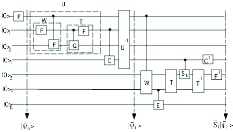
FIG. 1.: The quantum network for the construction of the state ${\tilde{S}}_{1}|{\bar{\psi}}_{0}>$. Selection of composites is done in $|{\bar{\psi}}_{1}>$, selection of Carmichaels is done in ${\tilde{S}}_{1}|{\bar{\psi}}_{0}>$. The operator $C$ is defined as $C\equiv 1-\Theta_{m+1}$.

In particular, one can show that the norm of the correction term $|E>$ in eq. (37) is upper bounded by

$$<E|E> = {4\over N}\biggl{[}\sum_{k_{co,C}}{\phi(k)\over k}\beta_{k}^{2}+\sum_{k_{co,NC}}{\phi(k)\over k}(1-\beta_{k}^{2})\alpha_{k}^{2}\biggr{]}$$ (39)

$$\leq {4\pi^{2}\over 3P^{2}}.$$ (40)

Moreover, it can be shown that the overall contribution to the state (37) coming from the bases $a$ for which $G_{k}(a)=1$ and the last ancilla qubit is in the state $|1>_{G}$, i.e. $|\Phi>\equiv|\Psi>+|E>$, has a norm $<\Phi|\Phi>=[\sum_{k=1}^{N}\phi(k)/k]/N\simeq\pi^{2}/6$.

Next, Grover’s transform $\tilde{G}$ entering the MAIN-LOOP of the algorithm, i.e. that counting the total number $t_{N}$ of $k_{C}<N$, can be written as

$$\tilde{G}\equiv U_{2}~{}{\tilde{S}}_{1}~{}~{}~{}~{};~{}~{}~{}~{}U_{2}\equiv-W^{(k)}S_{0}^{(k)}W^{(k)},$$ (41)

where now the operations $W^{(k)}$ and $S_{0}^{(k)}$ are acting on the states $|k>$.

Then, starting from $|{\bar{\psi}}_{0}>$ given by formula (28) and tensoring it with another flat superposition of ancilla states, i.e.

$$|{\bar{\psi}}_{2}>\equiv{1\over\sqrt{Q}}\sum_{m=0}^{Q-1}|m>_{5}|{\bar{\psi}}_{0}>,$$ (42)

acting on $|{\bar{\psi}}_{0}>$ with the $|m>_{5}$-’controlled’ ${\tilde{G}}^{m}$ and with $F$ on $|m>_{5}$, and exploiting the linearity of the unitary transformation ${\tilde{S}}_{1}$ when acting on $|\Phi>|1>_{G}$ and on $|REST>|0>_{G}$, after some elementary algebra we get (see ref. [6] for more details)

$$|{\bar{\psi}}_{3}> \equiv \biggl{[}{1\over 2}\sum_{n=0}^{Q-1}e^{i\pi n(1-1/Q)}|n>_{5}[e^{-i\pi f_{Q}}s^{(Q)}_{n-}$$ (43)

$$\times (i|G>+|B>)+e^{i\pi f_{Q}}s^{(Q)}_{n+}(-i|G>+|B>)]$$ (44)

$$+ {1\over Q}\sum_{m,n=0}^{Q-1}e^{2i\pi mn/Q}|n>_{5}|E_{m}>\biggr{]}|1>_{G}$$ (45)

$$+ {1\over Q}\sum_{m,n=0}^{Q-1}e^{2i\pi mn/Q}|n>_{5}$$ (46)

$$\times {\tilde{G}}^{m}|REST>|0>_{G},$$ (47)

where we have defined, similarly to section III,

$$\sin\theta_{N} \equiv \sqrt{t_{N}\over N}$$ (48)

$$f_{Q} \equiv {Q\theta_{N}\over\pi},$$ (49)

the ’good’ and ’bad’ states, respectively, as

$$|G> \equiv {\sum_{k_{C}}|k>|0>_{1,2}\over\sqrt{t_{N}}}$$ (50)

$$|B> \equiv {\sum_{k_{NC}}|k>|0>_{1,2}\over\sqrt{N-t_{N}}},$$ (51)

the ’error’ term as

$$|E_{n}>\equiv\sec\theta_{N}\left[\sum_{j=1}^{n}~{}l_{n-j}{\tilde{G}}^{j-1}\right]U_{2}|E>,$$ (52)

with $l_{j}\equiv\cos(2j+1)\theta_{N}$, and $s^{(Q)}_{n\pm}$ as in eq. (21).

Finally, we measure the last ancilla qubit $|\cdot>_{G}$. If we get $|0>_{G}$, we start again building the state $|{\bar{\psi}}_{0}>$ as in eq. (28). Otherwise, if we get $|1>_{G}$ (i.e., the part of $|{\bar{\psi}}_{3}>$ coming from the bases with $G_{k}(a)=1$), we can go on to the last step of the algorithm and further measure the first ancilla qubit $|\cdot>_{5}$ in $|{\bar{\psi}}_{3}>$. Using the expected estimate that $\theta_{N}\sim O[1/l(N)^{1+\epsilon/2}]$, and by choosing

$$Q\simeq O[l(N)^{\beta}]~{}~{}~{}~{};~{}~{}~{}~{}\beta>1+\epsilon/2,$$ (53)

we get the ansatz $1<f_{Q}<Q/2-1$, for which it can be shown [5] that the probability $\tilde{W}$ to obtain any of the states $|f_{-}>_{5}$, $|f_{+}>_{5}$, $|Q-f_{-}>_{5}$ or $|Q-f_{+}>_{5}$ in the final measurement is given by

$${\tilde{W}}\geq{8\over\pi^{2}}.$$ (54)

This means that with a high probability we will always be able to find one of the states $|f_{\pm}>_{5}$ or $|P-f_{\pm}>_{5}$ and, therefore, to evaluate the number $t_{N}$ from eq. (49).

Since in general $f_{Q}$ is not an integer, the measured ${\tilde{f}}_{Q}$ will not match exactly the true value of $f_{Q}$, and consequently (defining ${\tilde{t}}_{N}\equiv N\sin^{2}{\tilde{\theta}}_{N}$, with ${\tilde{\theta}}_{N}={\tilde{\theta}}_{N}({\tilde{f}}_{Q})$) we will have an error over $t_{N}$ [5] given by

$$|\Delta t_{N}|_{exp} \equiv |{\tilde{t}}_{N}-t_{N}|\leq\pi{N\over Q}\left[{\pi\over Q}+2\sqrt{t_{N}\over N}\right]$$ (55)

$$\simeq O\left[{N\over Q}~{}l(N)^{-(1+\epsilon/2)}\right].$$ (56)

Then, if we want to check the theoretical formula for $t_{N}$ with a precision up to some power $\delta$, with $0<\delta\ll\epsilon$ in $l(N)$, i.e. with

$$|\Delta t_{N}|_{th}\simeq O[N~{}l(N)^{-(2+\epsilon+\delta)}],$$ (57)

we have to impose that $|\Delta t_{N}|_{exp}<|\Delta t_{N}|_{th}$, which implies that we can take $Q$ as given by eq. (53) with $\beta>1+\epsilon/2+\delta$. The computational complexity of the quantum algorithm can be finally estimated as $S_{Q}\simeq O[QPS_{G}]\geq O[l(N)^{2+\epsilon+2\delta}]$, i.e. superpolynomial but still subexponential in $\log N$.

V Discussion

Our quantum algorithms testing and counting Carmichael numbers make essential use of some of the basic blocks of quantum networks known so far, i.e. Grover’s operator for the quantum search of a database [4], Shor’s Fourier transform for extracting the periodicity of a function [3] and their combination in the counting algorithm of ref. [5]. The most important feature of our quantum probabilistic algorithms is that the coin tossing used in the correspondent classical probabilistic ones is replaced here by a unitary and reversible operation, so that the quantum algorithm can even be used as a subroutine in larger and more complicated networks. Our quantum algorithm may also be useful for other similar tests and counting problems in number theory if there exists a classical probabilistic algorithm which somehow can guarantee a good success probability. Finally, it is known that in a classical computation one can count, by using Monte-Carlo methods, the cardinality of a set which satisfies some conditions, provided that the distribution of the elements of such a set is assumed to be known (e.g., homogeneous). One further crucial strength and novelty of our algorithm is also in the ability of efficiently and successfully solve problems where such a knowledge or regularities may not be present.

Acknowledgements

A.H.’s research was partially supported by the Ministry of Education, Science, Sports and Culture of Japan, under grant n. 09640341. A.C.’s research was supported by the EU under the Science and Technology Fellowship Programme in Japan, grant n. ERBIC17CT970007; he also thanks the cosmology group at Tokyo Institute of Technology for the kind hospitality during this work. Both authors would like to thank Prof. N. Kurokawa for helpful discussions.

REFERENCES

- [1] P. Benioff, Journ. Stat. Phys., 22, 563 (1980); D. Deutsch, Proc. Roy. Soc. London, Ser. A 400, 96 (1985); R.P. Feynman, Found. Phys., 16, 507 (1986).
- [2] D.P. DiVincenzo, Science, 270, 255 (1995); A. Steane, Rep. Prog. Phys., 61, 117 (1998).
- [3] P.W. Shor, in Proceedings of the 35th Annual Symposium on Foundations of Computer Science, ed. S. Goldwater (IEEE Computer Society Press, New York, 1994), p. 124; SIAM Journ. Comput., 26, 1484 (1997).
- [4] L.K. Grover, in Proceedings of the 28th Annual Symposium on the Theory of Computing (ACM Press, New York, 1996), p. 212; Phys. Rev. Lett., 79, 325 (1997).
- [5] G. Brassard, P. Hoyer and A. Tapp, Los Alamos e-print quant-ph/9805082; M. Boyer, G. Brassard, P. Hoyer and A. Tapp, in Proceedings of the 4th Workshop on Physics and Computation, ed. T. Toffoli et al. (New England Complex Systems Institute, Boston, 1996), p. 36; also in Los Alamos e-print quant-ph/9605034 (1996) and Fortsch. Phys., 46, 493 (1998).
- [6] A. Carlini and A. Hosoya, Los Alamos e-print quant-ph/9907020.
- [7] P. Ribenboim, The New Book of Prime Number Records (Springer-Verlag, New York, 1996).
- [8] R.D. Carmichael, Bull. Am. Math. Soc., 16, 232 (1910).
- [9] W.R. Alford, A. Granville and C. Pomerance, Ann. Math., 140, 703 (1994).
- [10] L. Monier, Theor. Comp. Sci., 12, 97 (1980).
- [11] R. Baillie and S.S. Wagstaff Jr., Math. Comp., 35, 1391 (1980).
- [12] P. Erdos and C. Pomerance, Math. Comp., 46, 259 (1986).
- [13] M.O. Rabin, Journ. Num. Th., 12, 128 (1980); also in Algorithms and Complexity, Recent Results and New Directions, ed. J.F. Traub (Academic Press, New York, 1976), p. 21; C.L. Miller, J. Comp. Syst. Sci., 13, 300 (1976).
- [14] C. Pomerance, J.L. Selfridge and J.J. Wagstaff Jr., Math. Comp., 35, 1003 (1980).
- [15] P. Erdos, Publ. Math. Debrecen., 4, 201 (1956).