Casimir force between metallic mirrors

Abstract

We study the influence of finite conductivity of metals on the Casimir effect. We put the emphasis on explicit theoretical evaluations which can help comparing experimental results with theory. The reduction of the Casimir force is evaluated for plane metallic plates. The reduction of the Casimir energy in the same configuration is also calculated. It can be used to infer the reduction of the force in the plane-sphere geometry through the ‘proximity theorem’. Frequency dependent dielectric response functions of the metals are represented either by the simple plasma model or, more accurately, by using the optical data known for the metals used in recent experiments, that is Al, Au and Cu. In the two latter cases, the results obtained here differ significantly from those published recently.

PACS: 03.70 +k, 12.20 Ds, 42.50 Lc

I Introduction

The Casimir force experienced by reflectors placed in vacuum is a macroscopic mechanical consequence of quantum fluctuations of electromagnetic fields [1]. Despite its relatively small magnitude, it has been observed in a number of ‘historic’ experiments [2, 3, 4, 5]. A much better experimental precision has been reached in recent experiments [6, 7] which should now allow for an accurate comparison with theory. Clearly this requires not only a detailed control of the experiments but also a careful theoretical estimation of the various corrections corresponding to the differences between real experiments and the idealized Casimir situation.

The present paper is focussed on the estimation of corrections associated with the non ideal behavior of metallic reflectors. Additional corrections due to the effect of non-zero temperature and the geometry of the cavity have also to be mastered before an agreement of experimental results with theoretical expectations can be claimed. A general discussion of the corrections to Casimir formulas is presented in the next section. In particular, we recall how the Casimir force measured in the plane-sphere geometry may be inferred from the Casimir energy in the plane-plane geometry by using the so-called ‘proximity theorem’.

We then focus attention on our main topic which is the evaluation of the reduction factor of Casimir force and Casimir energy for plane metallic plates in the limit of a large surface. We first compute the reduction factors obtained when describing the dielectric functions with a plasma model. This computation covers the whole range of distances large or small with respect to the plasma wavelength. The analytical expression of the force in the limit of small distances is also derived.

The plasma model is not a good description of the dielectric constant at low frequencies because it ignores the relaxation of electrons responsible for optical response of metals. This is why we also investigate the Drude model which accounts for this relaxation. We finally discuss in detail a more accurate description of the dielectric constant based on the optical data known for the metals. We concentrate on the three metals, Aluminium, Gold and Copper, used in recent experiments and give the reduction factors for the whole range of experimentally explored distances. For Au and Cu, we obtain results differing significantly from recently published ones [8].

II Corrections to the Casimir formula

In the original point of view [1], the Casimir effect is derived from the change of the total energy of vacuum due to the presence of two plane perfect reflectors. In this global approach, the Casimir energy is the part $E_{C}$ of vacuum energy depending on the plate separation $L$

$$E_{C}=A\frac{\hbar c\pi^{2}}{720L^{3}}$$ (1)

This energy is proportional to the surface $A$ of the reflectors in the limit of a large surface, the Planck constant $\hbar$ and the speed of light $c$. The Casimir force $F_{C}$ between the two reflectors is then derived from this position dependent energy

$$F_{C}=-\frac{{\rm d}E_{C}}{{\rm d}L}=A\frac{\hbar c\pi^{2}}{240L^{4}}$$ (2)

Being proportional to the surface, it defines a pressure which depends only on the distance $L$ and the two fundamental constants $\hbar$ and $c$. Conventions of sign have been chosen so that both numbers (1,2) are positive with the significance that the Casimir force is attractive and the Casimir energy is a binding energy.

In contrast with this global point of view, the Casimir force may also be understood as a local quantity, namely the radiation pressure exerted upon mirrors by vacuum fluctuations which are modified by the presence of the reflectors. This local approach makes it much easier to deal with corrections of Casimir formulas (1,2). In a remarkable work, Lifshitz gave a general formula for the Casimir force between two plane plates characterized by their dielectric response functions [9]. In particular his formula accounts for the finite reflectivity of metallic mirrors and it was used to deduce a first order correction for the plasma model of metals [10]. Since the dielectric constant is large at frequencies smaller than the plasma frequency $\omega_{P}$, the Casimir formula is recovered at distances larger than the plasma wavelength

$$\lambda_{P}=\frac{2\pi c}{\omega_{p}}$$ (3)

At frequencies larger than $\omega_{P}$ in contrast, the mirror has a poor reflectivity so that the force is reduced with respect to (2) at distances of the order of the plasma wavelength $\lambda_{P}$ which lies in the sub-$\mu$m range. The force may thus be written in terms of a factor $\eta_{F}$ which measures the reduction of the force with respect to the case of perfect mirrors

$$F=\eta_{F}F_{C}$$ (4)

The expression of the reduction factor is read at long distances as [11, 12]

$$\eta_{F}\simeq 1-\frac{8}{3\pi}\frac{\lambda_{P}}{L}\quad\Leftarrow\quad\frac{\lambda_{P}}{L}\ll 1$$ (5)

In the following we will also introduce a reduction factor $\eta_{E}$ for the Casimir energy $E$

$$E=\int_{L}^{\infty}F\left(x\right)~{}{\rm d}x=\eta_{E}E_{C}$$ (6)

The Lifshitz formula also contained thermal corrections to the Casimir effect usually studied at zero temperature. These corrections are significant at distances larger than or of the order of a typical length [9]

$$\lambda_{T}=\frac{\hbar c}{k_{B}T}$$ (7)

where $k_{B}$ is the Boltzmann constant and $T$ the temperature. At room temperature this length is of the order of a few $\mu$m. Hence thermal corrections become significant for distances for which the mirrors can be considered as nearly perfect reflectors. Well established estimations of thermal corrections for perfect mirrors may thus be used to evaluate the effect of temperature [12, 13, 14]. This effect is found to be negligible at distances smaller than 1 $\mu$m and to become dominant at distances larger than 5 $\mu$m [7, 15].

The Lifshitz formula has been derived for plane plates in the limit of large transverse surface and large longitudinal optical depth. But recent experiments have been performed in a plane-sphere geometry which makes easier the control of geometry and, in particular, the precise control of the distance between plates [6, 7]. Furthermore, mirrors are often built as multilayered structures rather than as single plates with a large optical depth. Finally the roughness of the metal/vacuum interfaces may also play an important role. These features have to be taken into account in an accurate estimation.

We will not present a detailed analysis of the geometrical effects in this paper. It is however worth recalling that the Casimir force in the plane-sphere geometry is usually estimated from the so-called ‘proximity theorem’. Basically this theorem amounts to evaluating the force by adding the contributions of various distances as if they were independent. In the plane-sphere geometry the force $F_{pt}$ evaluated from the proximity theorem is thus read as [16, 17, 18, 19]

$$F_{pt}=2\pi RE=2\pi R\eta_{E}E_{C}$$ (8)

where $R$ is the radius of the sphere and $E$ the Casimir energy evaluated in the plane-plane configuration for the same distance $L$, this distance being defined as the distance of closest approach in the plane-sphere geometry. Hence, the reduction factor $\eta_{E}$ for the Casimir energy evaluated in the plane-plane configuration in (6) can be used to infer the reduction factor for the force measured in the plane-sphere geometry through the proximity theorem.

At this point we have to emphasize that our calculations are intended to provide a reliable estimation of the Casimir force and energy between two metal plates in the plane-plane geometry. Clearly, they do not give any indication of the degree of reliability of the proximity theorem. Since it is well known that the Casimir force is not an additive quantity one cannot but question an estimation based on an addition procedure [20]. Precisely, one can hardly admit that the proximity theorem provides reliable estimations at the level of accuracy which is now aimed at, that is the % level. As already discussed, these problems are not the main task of this paper which is focussed on the effect of imperfect reflection of metallic mirrors. The same remarks apply to another aspect of the geometry, that is the roughness effect which has also been found to play a significant role [19, 21].

III The description of mirrors

As predicted by Casimir in his founding article [1] the divergences associated with the infiniteness of vacuum energy do not play a real role in the estimation of Casimir effect thanks to a general physical reason: real mirrors are certainly transparent at the limit of infinite frequencies. This idea was implemented in the Lifshitz theory [9] and it has a much broader range of validity. Real mirrors may always be characterized by frequency dependent reflectivity amplitudes which provide a finite expression for Casimir energy as soon as general properties of unitarity, causality and high-frequency transparency are accounted for [22]. Dispersive optical response functions necessarily include dissipation mechanisms so that incoming electromagnetic fields and additional Langevin fluctuations coming from matter have to be treated simultaneously [23]. The description of mirrors through well behaved reflectivity amplitudes [22] automatically includes a proper description of these fluctuations [24].

The two mirrors form a Fabry-Pérot cavity which enhances or decreases field fluctuations depending on whether their frequency is resonant or not with cavity modes. This modulation of intracavity energy of vacuum fluctuations, integrated over frequencies and incidence angles corresponding to the various modes, is responsible for the Casimir force [22]. Using causality properties, the force can be written as an integral over imaginary frequencies and wavevectors [9]. After these transformations, the Casimir force may be written in terms of a reduction factor (4) which takes the following form adapted from [22]

$$\eta_{F}=\frac{120}{\pi^{4}}\int_{0}^{\infty}{\rm d}KK^{2}\int_{0}^{K}{\rm d}\Omega\sum_{p}\frac{r_{p}^{2}}{e^{2K}-r_{p}^{2}}$$ (9)

$$K=\kappa L\qquad\Omega=\omega\frac{L}{c}$$ (10)

$r_{p}$ denotes the reflection amplitude for one of the two mirrors and a given polarization $p$. This notation is a shorthand for $r_{p}\left(i\omega,i\kappa\right)$ where $i\omega$ is the imaginary frequency and $i\kappa$ the imaginary wavevector along the longitudinal direction of the Fabry-Pérot cavity. $\Omega$ and $K$ stand for the frequency and wavevector measured in dimensionless units with the help of the cavity length $L$. The reflection amplitudes are supposed to be identical for the two mirrors. Otherwise $r_{p}^{2}$ has to be replaced by the product of the two amplitude reflection coefficients.

In the limit of perfect mirrors $\left(r_{p}^{2}=1\right)$ the Casimir formula (2) is recovered $\left(\eta_{F}=1\right)$. In the general case, the factor $\eta_{F}$ measures the reduction of the force between real mirrors with respect to the case of perfect mirrors. We may also write a reduction factor (6) for the Casimir energy

$$\eta_{E}=-\frac{180}{\pi^{4}}\int_{0}^{\infty}{\rm d}KK\int_{0}^{K}{\rm d}\Omega\sum_{p}{\rm Log}\left(1-r_{p}^{2}e^{-2K}\right)$$ (11)

Let us stress again that the expressions (10,11) give only the corrections to Casimir force and energy associated with the finite conductivity of metallic plates. They correspond to plane reflecting plates at the limit of a large surface, assume a null temperature and disregard the problem of roughness. As discussed in the previous section, the factor $\eta_{E}$ may be used to infer the force in the plane-sphere geometry through the proximity theorem.

Assuming furthermore that the metal plates have a large optical thickness, the reflection coefficients $r_{p}$ correspond to the ones of a mere vacuum-metal interface [25]

$$r_{\bot} = -\frac{\sqrt{\omega^{2}\left(\varepsilon\left(i\omega\right)-1\right)+c^{2}\kappa^{2}}-c\kappa}{\sqrt{\omega^{2}\left(\varepsilon\left(i\omega\right)-1\right)+c^{2}\kappa^{2}}+c\kappa}$$ (12)

$$r_{||} = \frac{\sqrt{\omega^{2}\left(\varepsilon\left(i\omega\right)-1\right)+c^{2}\kappa^{2}}-c\kappa\varepsilon\left(i\omega\right)}{\sqrt{\omega^{2}\left(\varepsilon\left(i\omega\right)-1\right)+c^{2}\kappa^{2}}+c\kappa\varepsilon\left(i\omega\right)}$$ (13)

$r_{p}$ still stands for $r_{p}\left(i\omega,i\kappa\right)$ and $\varepsilon\left(i\omega\right)$ is the dielectric constant of the metal evaluated for imaginary frequencies. Taken together, the relations (10,13) reproduce the Lifshitz expression for the Casimir force [9]. We however emphasize that (10) can be used to go beyond the Lifshitz expression since it allows one to deal with more general mirrors than those considered in (13).

As an example we consider mirrors built as metallic slabs having a finite thickness. For a given polarization, we denote by $\rho$ the reflection coefficient (13) corresponding to a single vacuum/metal interface and we write the reflection amplitude $r$ for the slab of finite thickness through a Fabry-Pérot formula

$$r = \rho\frac{1-e^{-2\delta}}{1-\rho^{2}e^{-2\delta}}$$ (14)

$$\delta = \frac{D}{c}\sqrt{\omega^{2}\left(\varepsilon\left(i\omega\right)-1\right)+c^{2}\kappa^{2}}$$ (15)

This expression has been written directly for imaginary frequencies. The parameter $\delta$ represents the optical length in the metallic slab and $D$ the physical thickness. The single interface expression (13) is recovered in the limit of a large optical thickness $\delta\gg 1$. With the plasma model, this condition just means that the thickness $D$ is larger than the plasma wavelength $\lambda_{P}$.

In order to discuss recent experiments it may be useful to write the reflection coefficients for multilayer mirrors. For example one may consider two-layer mirrors with a layer of thickness $D$ of a metal $A$ deposited on a large slab of metal $B$ in the limit of large thickness. The reflection formulas are then obtained as in [26] but accounting for oblique incidence. The equations (10,11) may then be calculated for the two-layer mirrors. This could help to obtain more accurate estimations for the experiments as soon as physical characteristics of the two-layer mirrors are precisely known. In the present paper we use reflection amplitudes (13) which are well adapted to a general discussion since they depend on a smaller number of parameters.

IV Plasma and Drude model

We will now evaluate the reduction factor for the Casimir force when the frequency dependent dielectric function may be represented by the plasma or Drude models.

We begin with the plasma model where the quantities $\varepsilon\left(\omega\right)$ and $\varepsilon\left(i\omega\right)$ are represented as follows

$$\varepsilon\left(\omega\right) = 1-\frac{\omega_{P}^{2}}{\omega^{2}}$$ (16)

$$\varepsilon\left(i\omega\right) = 1+\frac{\omega_{P}^{2}}{\omega^{2}}$$ (17)

Using expressions (13,17) it is possible to obtain the reduction factor (10) defined for the Casimir force through numerical integrations. The result is drawn on figure 1, as a function of the dimensionless parameter $\frac{L}{\lambda_{P}}$, that is the ratio between the distance $L$ and the plasma wavelength $\lambda_{P}$. As expected the Casimir formula is reproduced at large distances ($\eta_{F}\rightarrow 1$ when $\frac{L}{\lambda_{P}}\gg 1$). At distances smaller than $\lambda_{P}$ in contrast, a significant reduction factor is obtained. This factor $\eta_{F}$ scales as $\frac{L}{\lambda_{P}}$ at the limit of small distances. This means that the whole expression (4) of the Casimir force is a power law which undergoes a change of exponent when the distance $L$ crosses the plasma wavelength $\lambda_{P}$ characterizing the optical response of metals. This is quite analogous to the crossover discovered by Casimir and Polder for the variation of Van der Waals force with respect to the interatomic distance [27].

FIG. 1.: Reduction of the Casimir force compared to the force between perfect mirrors, when the finite conductivity may be described by a plasma model (solid line) or a Drude model (dashed line) with a ratio $\frac{\gamma}{\omega_{P}}$ equal to $4\times 10^{-3}$. The difference due to the relaxation parameter has only a small effect on the calculation of the Casimir force. The dotted-dashed line corresponds to the short distance asymptotic behavior.

An asymptotic law of variation for $\eta_{F}$ varying as $\frac{L}{\lambda_{P}}$ at small distances has been proposed repeatedly since Lifshitz [9]. We have been able to derive from (10,13,17) a precise value for the coefficient appearing in this law

$$L \ll \lambda_{P}\quad\rightarrow\quad\eta_{F}=\alpha\frac{L}{\lambda_{P}}$$ (18)

$$\alpha = \frac{30}{\pi^{2}}\int_{0}^{\infty}{\rm d}K~{}e^{-\frac{3K}{4}}\left(\frac{K^{2}}{\sqrt{\sinh\frac{K}{2}}}-\frac{K^{2}}{\sqrt{\cosh\frac{K}{2}}}\right)$$ (19)

$$\simeq 1.193$$ (20)

This implies a similar behavior for the reduction factor $\eta_{E}$ with a different proportionality coefficient

$$L\ll\lambda_{P}\quad\rightarrow\quad\eta_{E}=\frac{3}{2}\alpha\frac{L}{\lambda_{P}}$$ (21)

Hence, $\eta_{E}$ is larger than $\eta_{F}$ at short distances, which means a less important reduction with respect to the case of perfect mirrors. The asymptotic law (20) valid at short distances, taken with its equivalent (5) at large distances, is an important feature of the variation of $\eta_{F}$ with $L$ which is not obeyed by the approximants which have been used to discuss recent experimental results [8, 15]. These approximants are compared with the exact expression of the reduction factor for the plasma model in Appendix A.

As already discussed, the plasma model does not provide a good description of the dielectric response of metals. The main reason is that the dielectric function $\varepsilon\left(\omega\right)$ is real in (17) and, therefore, does not account for any dissipative mechanism. A much better representation of the dielectric function corresponding to the optical response of conduction electrons is the Drude model [28]

$$\varepsilon\left(\omega\right) = 1-\frac{\omega_{P}^{2}}{\omega\left(\omega+i\gamma\right)}$$ (22)

$$\varepsilon\left(i\omega\right) = 1+\frac{\omega_{P}^{2}}{\omega\left(\omega+\gamma\right)}$$ (23)

This model describes not only the plasma response of conduction electrons with $\omega_{P}$ still interpreted as the plasma frequency but also their relaxation, $\gamma$ being the inverse of the electronic relaxation time.

The relaxation parameter $\gamma$ is much smaller than the plasma frequency. For Al, Au, Cu in particular, we will find in the next section values for the ratio $\frac{\gamma}{\omega_{P}}$ of the order of $4\times 10^{-3}$. Hence relaxation plays a significant role in the modeling of the dielectric constant only at frequencies where the latter is much larger than unity. Stated in different words, it has to be taken into account only when the metallic mirror behaves as a nearly perfect reflector. This suggests that the relaxation will not have a large influence on the Casimir effect. This qualitative argument is confirmed by the result of a numerical integration reported on figure 1. With a value of $\frac{\gamma}{\omega_{P}}$ equal to $4\times 10^{-3}$, that is of the order of the real values obtained for Al, Au, Cu, the variation of $\eta_{F}$ remains smaller than 2%. It thus plays a marginal role at the level of accuracy aimed at but it is easy and safer to take it into account.

V Real metals

For metals like Al, Au, Cu, the dielectric constant departs from the Drude model when interband transitions are reached, that is when the photon energy reaches a few $e$V. Hence, a more precise description of the dielectric constant, taking into account the known data on optical properties of these metals, has to be used for evaluating the force in the sub-$\mu$m range.

The dielectric response function for real frequencies may be written in terms of real and imaginary parts $\varepsilon^{\prime}$ and $\varepsilon^{\prime\prime}$ obeying general causality relations

$$\varepsilon\left(\omega\right) = \varepsilon^{\prime}\left(\omega\right)+i\varepsilon^{\prime\prime}\left(\omega\right)$$ (24)

$$\varepsilon^{\prime}\left(\omega\right)-1 = \frac{2}{\pi}{\cal P}\int_{0}^{\infty}\frac{x\varepsilon^{\prime\prime}\left(x\right)}{x^{2}-\omega^{2}}{\rm d}x$$ (25)

Causality relations also allow one to obtain the dielectric constant at imaginary frequencies $\varepsilon\left(i\omega\right)$ from the function $\varepsilon^{\prime\prime}\left(x\right)$ evaluated at real frequencies $x$, that is also the oscillator strength characterizing the material [29]

$$\varepsilon\left(i\omega\right)-1=\frac{2}{\pi}\int_{0}^{\infty}\frac{x\varepsilon^{\prime\prime}\left(x\right)}{x^{2}+\omega^{2}}{\rm d}x$$ (26)

When discussing optical data, we will measure frequencies either in $e$V or in rad/s, using the equivalence 1 $e$V $=1.537\times 10^{15}$ rad/s.

The values of the complex index of refraction, measured through different optical techniques, are tabulated as a function of frequency in several references [30, 31, 32]. Optical data may vary from one reference to another. Available data do not cover the whole frequency range and they have to be extrapolated. These two problems may cause variations of the results obtained for $\varepsilon\left(i\omega\right)$ and, therefore, for the Casimir force. This is why we explain in detail how we proceed from the input, the optical data, to the output of the process, the reduction factors for Casimir force and energy.

Figure 2 shows the values for $\varepsilon^{\prime\prime}(\omega)$ as a function of frequency $\omega$ for the three metals Al, Au and Cu. All data are taken from [30, 31] with a frequency range $0.04-1000~{}e$V for Al and $0.1-1000~{}e$V for Au and Cu. A large number of points is available in these sources so that the interpolation between these points does not raise any difficulty. However the data have to be extrapolated at low frequencies to increase the domain over which the integrations are performed. At energies around $0.1~{}e$V the optical properties are quite well described by the contribution of conduction electrons. Hence data available at these energies may be nicely fitted with a Drude model. For Al the corresponding Drude parameters are given in [30] as $\omega_{P}=11.5~{}e$V and $\gamma=50$ m$e$V. For Au and Cu there are not enough optical data at low frequencies to permit a determination of the two parameters $\omega_{P}$ and $\gamma$ separately. Here we use additional information namely the estimation of $\omega_{P}$ coming from solid state physics [28, 29]. Precisely we write

$$\omega_{P}^{2} = \frac{4\pi Ne^{2}}{m^{*}}=\frac{Nq^{2}}{\varepsilon_{0}m^{*}}$$ (27)

$$N = ZN_{a}$$ (28)

where $N$ is the number of conduction electrons per unit volume, that is also the product of the number $Z$ of electrons per atom by the atomic number density $N_{a}$, $q$ is the charge of electron and $m^{*}$ is the effective mass of conduction electrons. This mass is different of the mass $m$ of free electrons. The same correction may be described as a change of the effective number of conduction electrons per atom from $Z$ to $Z^{*}$. We keep the former description, use $Z=1$ for Cu and Au, and choose for effective masses of conduction electrons the values $\frac{m^{*}}{m}\simeq 1$ for Au and $\frac{m^{*}}{m}\simeq 1.45$ for Cu [33, 34].

FIG. 2.: The imaginary part of the dielectric constant as a function of real frequency (upper graph) and the dielectric constant as function of imaginary frequency (lower graph) for Al (solid line), Au (dotted line) and Cu (dashed line). At low frequencies the data fit a Drude model corresponding to the contribution of conduction electrons. Peaks in the imaginary part of the dielectric function correspond to deviations from the Drude model associated with interband transitions.

With these assumptions we obtain nearly equal values for the plasma frequency of Au and Cu, $\omega_{P}=9.0~{}e$V. This corresponds to a plasma wavelength of 136 nm for Au and Cu, to be compared with the plasma wavelength of 107 nm for Al. Then the optical data of [30] allow us to deduce the relaxation parameter $\gamma$ fitting the low energy data points with a Drude model. We obtain in this manner $\gamma=35$ m$e$V for Au and $\gamma=30$ m$e$V for Cu. These values correspond respectively to $\frac{\gamma}{\omega_{P}}=3.8\times 10^{-3}$ and $\frac{\gamma}{\omega_{P}}=3.3\times 10^{-3}$ to be compared to $\frac{\gamma}{\omega_{P}}=4.4\times 10^{-3}$ for Al. Note that we have given deliberately all the numerical values in this paragraph with a limited accuracy since slightly different values could have been obtained as well, starting from different sources or using different criteria for choosing the values. This problem of extrapolation of optical data at low frequencies is certainly a cause for systematical errors in the estimation of the Casimir force.

The dielectric constant for imaginary frequencies $\varepsilon\left(i\omega\right)$ is then obtained by numerical integration of relation (26). Of course, the integration cannot be performed over the whole range $[0,\infty]$ of frequencies so that we have to give details about the integration procedure. We are mainly interested in experimentally explored plate separations in the range $0.1-10~{}\mu$m. These separations correspond to frequencies in the range $0.1-10~{}e$V. We thus need reliable values for $\varepsilon(i\omega)$ with $\omega$ ranging from $10^{-4}$ to $10^{3}~{}e$V. To this aim we have to integrate (26) over real frequencies covering a still broader range $10^{-6}-10^{4}~{}e$V. In order to test the integration procedure we have varied the integration range by half an order of magnitude which changed the result by less than 1 %. The curves obtained for the three metals are shown in the lower graph of figure 2. In particular the curves for Au and Cu are nearly identical over the whole range of frequencies.

The Casimir force and energy are then calculated by numerical integration of equations (10,11). The integration range is chosen as $10^{-4}-10^{3}~{}e$V in order to evaluate the Casimir force for plate separations in the range $0.1-10~{}\mu$m. The same test of the integration procedure has been performed leading to an error less than 1.5% for $\eta_{F}$ and 2% for $\eta_{E}$. The limit of perfect reflectors has been reproduced with an error less than 1%. Figure 3 shows the reduction of the Casimir force and energy between metallic mirrors with respect to perfectly reflecting mirrors for the three metals. The force is reduced when going from Al to Au and has nearly the same value for Au and Cu. This directly reflects the behavior of the

FIG. 3.: Reduction of the Casimir force (upper graph) and energy (lower graph) between metallic reflectors with respect to perfectly reflecting mirrors as a function of their distance $L$. The three curves correspond to Al (solid line), Au (dotted line) and Cu (dashed line).

dielectric constants $\varepsilon(i\omega)$ which decrease along the same series on figure 2. As already discussed in the previous section the reduction $\eta_{E}$ is less pronounced than $\eta_{F}$.

We give in the following table a few numerical values for the reduction factors $\eta_{F}$ and $\eta_{E}$ for the three metals at three typical distances

$$\begin{array}[]{cccc}&\quad{\rm Al}&\quad{\rm Au}&\quad{\rm Cu}\\ \eta_{F}\left[0.1~{}\mu{\rm m}\right]&0.55&0.48&0.48\\ \eta_{E}\left[0.1~{}\mu{\rm m}\right]&0.63&0.55&0.55\\ \eta_{F}\left[0.5~{}\mu{\rm m}\right]&0.85&0.81&0.81\\ \eta_{E}\left[0.5~{}\mu{\rm m}\right]&0.88&0.85&0.85\\ \eta_{F}\left[3.0~{}\mu{\rm m}\right]&0.96&0.96&0.96\\ \eta_{E}\left[3.0~{}\mu{\rm m}\right]&0.97&0.97&0.97\end{array}$$ (29)

We remind once again that $\eta_{E}$ is the reduction factor for energy between two plane mirrors, that is also the estimate of reduction factor for the force in the plane-sphere geometry. From our analysis the factors $\eta_{F}$ and $\eta_{E}$ turn out to be the same for Au and Cu. Incidentally, as the dielectric constants of Au and Cu are nearly the same, mirrors built with a layer of Au on a slab of Cu would not lead to different results. This seems to solve a difficulty in the analysis of experimental results of [6]. The values obtained here for Al at $0.1~{}\mu{\rm m}$ and Cu at $0.5~{}\mu{\rm m}$ correspond to those found in [8]. But significant differences appear for Au at $0.5~{}\mu{\rm m}$ where we find values of $\eta_{F}$ and $\eta_{E}$ exceeding by 23% and 18% respectively the values given in [8]. Furthermore the agreement between our result for Cu at $0.5~{}\mu{\rm m}$ and the one in [8] appears to be an accidental crossing between two curves having quite different behaviors as functions of distances. Since these differences have important consequences for the comparison of experimental results with theory, we discuss them in detail in Appendix B.

VI Conclusion

The Casimir force has now been experimentally explored at distances in the sub-$\mu$m range and the reduction of the force due to finite conductivity of metals has been observed. For an accurate comparison of the experimental results with theory, it is necessary to dispose of precise theoretical expectations.

In this paper we have presented a detailed analysis of the influence of the imperfect reflection on the Casimir force between two plane metallic plates. In particular, we have given a precise evaluation of the reduction factor for metals used in recent experiments, that is Al, Au and Cu. This factor becomes significant at distances smaller than $1~{}\mu$m and it reaches values of about 50% for the smallest explored distances.

The reduction factor $\eta_{E}$ calculated in the present paper for the energy between plane plates can be used to infer the reduction factor for the force in the plane-sphere geometry if the proximity theorem is trusted. However the accuracy of this theorem is not known. Other corrections have also to be taken into account. Thermal corrections are significant at distances larger than a few $\mu$m but have not been seen in the experiment where these distances were explored [6]. The roughness corrections are also expected to play an important role [19, 21].

In these conditions it is premature to claim that a good agreement has been reached between experiments and theory. It is worth developing new experiments using either the same techniques or different ones [35, 36]. More work is also needed on the theoretical side, in particular for obtaining more reliable estimations of the effect of geometry and roughness on the Casimir force. Such efforts are certainly worthwhile not only because of the interest of reaching conclusions on the Casimir force but also for making it possible to control its effect when studying small short range forces [37, 38, 39, 40].

Acknowledgements We wish to thank Ephraim Fischbach, Marc-Thierry Jaekel, David Koltick, Vladimir Mostepanenko and Roberto Onofrio for stimulating discussions.

A The plasma corrections

In this appendix we compare the reduction factor $\eta_{F}$ evaluated for the Casimir force from expressions (10,13) using the plasma model (17) with different approximants which have been used to discuss recent experimental results (see for example [8, 15, 19]).

The exact result is the solid line of figure 1 reproduced as the solid line on figure 4. Its behavior at long distances $\left(L\gg\lambda_{P}\right)$ corresponds to the known development [18]

$$\eta_{A}=1-\frac{8}{3\pi}\frac{\lambda_{P}}{L}+\frac{6}{\pi^{2}}\left(\frac{\lambda_{P}}{L}\right)^{2}$$ (A1)

drawn as long dashes A on figure 4. Another interpolation formula may be deduced from this behavior as [18]

$$\eta_{B}=\left(1+\frac{11}{6\pi}\frac{\lambda_{P}}{L}\right)^{-\frac{16}{11}}$$ (A2)

This formula, drawn as short dashes B on figure 4, presents the advantage of being positive at all distances and also being a monotonic function of distance, two important features of the exact result. However it fails to reproduce the asymptotic variation of $\eta_{F}$ at small distances (compare with (20)). Another approximant, obtained by developing $\eta_{B}$ at the fourth order in $\frac{\lambda_{P}}{L}$, has sometimes been used [15]

$$\eta_{C} = \eta_{A}-\frac{38}{3\pi^{3}}\left(\frac{\lambda_{P}}{L}\right)^{3}+\frac{931}{9\pi^{4}}\left(\frac{\lambda_{P}}{L}\right)^{4}$$ (A3)

It is drawn as the dotted-dashed line C on figure 4. On the whole, figure 4 clearly shows that all these approximants fail to reproduce the correct behavior at distances smaller than the plasma wavelength $\lambda_{P}$.

FIG. 4.: Reduction factor $\eta_{F}$ for the Casimir force as a function of the ratio $\frac{L}{\lambda_{P}}$ when the finite conductivity is described by a plasma model (solid line). This curve is compared to different approximants (dashed lines) used in the literature and described in the text. These approximants are reasonable at large distances but depart from the exact result when $\frac{L}{\lambda_{P}}$ approaches unity.

Incidentally an interesting approximant may be defined by the following formula

$$\eta_{U}=\frac{1}{1+\frac{8}{3\pi}\frac{\lambda_{P}}{L}}$$ (A4)

It fits the known behavior of the exact result at the first-order, but not the second-order one, in $\frac{\lambda_{P}}{L}$. It is proportional to $\frac{L}{\lambda_{P}}$ at small distances as the correct result (20). Moreover the coefficient $\frac{3\pi}{8}$ has a value $1.178$ very close to the proportionality coefficient $\alpha\simeq 1.193$ appearing in (20), the relative difference being of the order of 1%. Hence, $\eta_{U}$ may be considered as a uniform approximant reproducing the variation of $\eta_{F}$ over the whole range of distances. It reproduces the exact result everywhere with an error of at most 5%. This precision is however not sufficient for it to be used in the place of the correct result.

B The case of Copper

In this appendix, we compare the reduction factors $\eta_{F}$ and $\eta_{E}$ obtained for Copper from the computations of the present paper and those of [8]. Both derivations are based on the same procedure which we have already described in the text. Optical data taken from different references agree reasonably well between each other. We however point out that quite different techniques are used here and in [8] for interpolating between available data and extrapolating at low frequencies and that these differences are responsible for significant deviations in the behaviors of $\eta_{F}$ and $\eta_{E}$ as functions of the plate separation.

The upper graph of figure 5 shows three different plots of the imaginary part of the dielectric constant. The first one is the one explained in the present paper with data points taken from [30, 31] (diamonds) and extrapolation at low frequency with a Drude model (solid line on figure 5). Our procedure is explained in more detail in the main part of this paper. The corresponding Drude parameters, a plasma frequency $\omega_{P}=9.0~{}e$V and a relaxation parameter $\gamma=30$ m$e$V are in reasonable agreement with existing knowledge from solid state physics.

The second plot has been designed by ourselves as an attempt to reproduce the computations of [8]. The triangles are optical data taken from [32]. These data are not exactly identical but they are in reasonable agreement with those taken from [30, 31]. However only three data points are given in [32] for the frequency range $10^{14}$-$2\times 10^{15}$ rad/s whereas a much larger number of data points may be found in [30, 31]. In contrast to our treatment, a specific interpolation procedure had therefore to be used in [8] to fill the gaps between the data points. Although this procedure is not described explicitly in [8] we have been able to reproduce a curve having the same appearance (compare with figure 1a in [8]). This curve results from a linear interpolation between the data points on a lin-lin scale. It appears clearly on figure 5 that this interpolation procedure produces bumps on the dielectric response functions (dashed line) which are largely outside the data known from [30, 31]. Optical data are in fact consistent with a linear interpolation on a log-log scale rather than on a lin-lin scale. This is the first important difference between the two treatments. The second important difference is associated with the extrapolation of data at low frequencies. In [8] the data points were extrapolated by a power law proportional to $1/\omega$ starting from the lowest frequency data available in [32]. The whole curve of [8] is not at all consistent with a Drude model at frequencies below $10^{15}$ rad/s. To summarize this presentation of the dielectric function used in [8] we may say that it corresponds to values too large in the range $10^{14}$-$2\times 10^{15}$ rad/s by a factor which can be more than $10$ and too small below $10^{14}$ rad/s by a factor up to $6$.

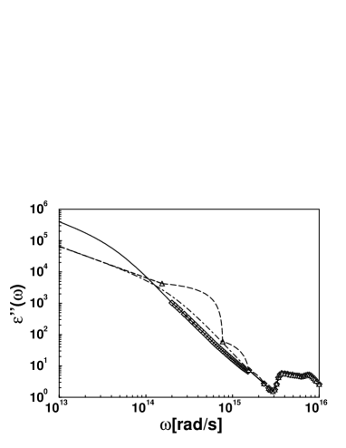
FIG. 5.: Imaginary part of the dielectric constant as a function of frequency (upper graph) and dielectric constant as function of imaginary frequency (lower graph) for Copper. The diamonds are data points from reference [30, 31] and the solid line is our extrapolation at low frequencies of these data. The triangles correspond to data points from [32]. The dashed line represents the extrapolation at low frequencies and the interpolation between the last three data points as in [8]. The dotted-dashed line corresponds to another extrapolation of the same data. More detailed explanations are given in the text.

The case of low frequency extrapolation requires more cautious discussions. As explained in the main part of this paper, the optical data available for Cu do not permit an unambiguous estimation of the two parameters $\omega_{P}$ and $\gamma$ separately. Other couples of value can be chosen which would also be consistent with optical data. To make this point explicit, we have drawn a third plot on figure 5 (dashed-dotted line) which corresponds to a Drude model fitting the optical data of [32] and the low frequency behavior of [8]. Obviously it does not reproduce the extra bumps of [8]. The associated Drude paramaters $\omega_{P}=7.5~{}e$V and $\gamma=130$ m$e$V correspond to an effective mass $\frac{m^{*}}{m}\simeq 2.1$ and to a ratio $\frac{\gamma}{\omega_{P}}\simeq 1.7\times 10^{-2}$ which are quite different from those used in our treatment. In order to have an indication of the effect of the uncertainties associated with optical data, we will however proceed to the computations with this curve, too.

We now perform the calculations as explained in the main part of the text. The lower graph on figure 5 shows the different results for the dielectric constant $\varepsilon(i\omega)$ as a function of imaginary frequency for the three different dielectric functions. As expected from the previous discussion, the values $\varepsilon(i\omega)$ found in [8] are too small at frequencies lower than $10^{14}$ rad/s but too large around $10^{15}$ rad/s when compared to those deduced from our calculation. This has a significant consequence for the evaluation of the reduction factors $\eta_{F}$ and $\eta_{E}$ drawn on figure 6 for a plate separation ranging from $0.1~{}\mu$m to $10~{}\mu$m.

FIG. 6.: Reduction factors $\eta_{F}$ for the Casimir force (upper graph) and $\eta_{E}$ for the Casimir energy (lower graph) as a function of the plate separation $L$. The solid line corresponds to the calculation of the present paper, the dashed line to the calculation in [8]. The dotted-dashed line corresponds to a calculation with a Drude model fitting the optical data of [32] and the low frequency behavior of [8].

Our reconstruction of the computations of [8] reproduce pretty well the published results at the distance of $0.5~{}\mu{\rm m}$ for which numerical values are given. However, the general behaviors of the curves are quite different. The Casimir force and Casimir energy obtained from the optical data used in [8] are too large at small distances and too small at large distances. These features, which are made explicit with values of $\eta_{E}$ given in the following table, are consistent with the discussions of the preceding paragraphs. The three columns 1, 2, 3 correspond respectively to the solid lines, dashed lines and dotted-dashed lines of figures 5-6

$$\begin{array}[]{cccc}&\quad{\rm 1}&\quad{\rm 2}&\quad{\rm 3}\\ \eta_{E}\left[0.1~{}\mu{\rm m}\right]&0.55&0.60&0.49\\ \eta_{E}\left[0.5~{}\mu{\rm m}\right]&0.85&0.85&0.79\\ \eta_{E}\left[3.0~{}\mu{\rm m}\right]&0.97&0.94&0.93\end{array}$$ (B1)

The crossing of the results in columns 1 and 2 at the distance of $0.5~{}\mu$m appears as an accidental compensation of these two flaws. The relative difference between the two results may be as large as 10%.

A claim of agreement between experiment and theory could be based on a comparison of values of $\eta_{E}$ obtained at different distances with values in the column 1 or, perhaps, in the column 3. As explained above, both columns correspond to reasonable extrapolations of the optical data. The advantage of column 1 over column 3 lies in values of the Drude parameters in better accordance with the knowledge in solid state physics. The difference between columns 1 and 3 may be considered as giving an idea of the uncertainties associated with the incompleteness of optical data. In any case the two corresponding curves, drawn as solid and dotted-dashed lines on figure 6, have similar dependences on the plate separation although the absolute values are shifted from one curve to the other. In contrast the dashed curve on figure 6 which corresponds to the calculations of [8] and crosses the two former curves cannot be considered as consistent with the known optical data.

REFERENCES

- [1] H.B.G. Casimir, Proc. Kon. Nederl. Akad. Wet. 51 793 (1948)
- [2] B.V. Deriagin and I.I. Abrikosova, Soviet Physics JETP 3 819 (1957)
- [3] M.J. Sparnaay, Physica XXIV 751 (1958); W. Black, J.G.V. De Jongh, J.Th.G. Overbeek and M.J. Sparnaay, Transactions of the Faraday Society 56 1597 (1960)
- [4] D. Tabor and R.H.S. Winterton, Nature 219 1120 (1968)
- [5] E.S. Sabisky and C.H. Anderson, Phys. Rev. A7 790 (1973)
- [6] S.K. Lamoreaux, Phys. Rev. Lett. 78 5 (1997); erratum in Phys. Rev. Lett. 81 5475 (1998)
- [7] U. Mohideen and A. Roy, Phys. Rev. Lett. 81 4549 (1998); A. Roy, C. Lin and U. Mohideen, preprint xxx quant-ph/9906062
- [8] S.K. Lamoreaux, Phys. Rev. A59 R3149 (1999)
- [9] E.M. Lifshitz, Sov. Phys. JETP 2 73 (1956); E.M. Lifshitz and L.P. Pitaevskii, Landau and Lifshitz Course of Theoretical Physics: Statistical Physics Part 2 ch VIII (Butterworth-Heinemann, 1980)
- [10] N.E. Dzyaloshinshii, E.M. Lifshitz and L.P. Pitaevskii, Sov. Phys. Uspekhi 4 153 (1961)
- [11] C.M. Hargreaves, Proc. Kon. Nederl. Akad. Wet. B68 231 (1965)
- [12] J. Schwinger, L.L. de Raad Jr., and K.A. Milton, Annals of Physics 115 1 (1978)
- [13] J. Mehra, Physica 57 147 (1967)
- [14] L.S. Brown and G.J. Maclay, Phys. Rev. 184 1272 (1969)
- [15] G.L. Klimchitskaya, A. Roy, U. Mohideen and V.M. Mostepanenko, Phys. Rev. A, to appear
- [16] B.V. Deriagin, I.I. Abrikosova and E.M. Lifshitz, Quart. Rev. 10, 295 (1968)
- [17] J. Blocki, J. Randrup, W.J. Swiatecki and C.F. Tsang, Ann. Physics 105, 427 (1977)
- [18] V.M. Mostepanenko and N.N. Trunov Sov. J. Nucl. Phys. 42 812 (1985)
- [19] V.B. Bezerra, G.L. Klimchitskaya and C. Romero, Mod. Phys. Lett. 12, 2613 (1997)
- [20] C.R. Hagen, preprint xxx hep-th/9902057
- [21] A. Roy and U. Mohideen, Phys. Rev. Lett. 82, 4380 (1999)
- [22] M.T. Jaekel and S. Reynaud, J. Physique I-1 1395 (1991)
- [23] D. Kupiszewska, Phys. Rev. A46 2286 (1992)
- [24] S.M. Barnett, C.R. Gilson, B. Huttner and N. Imoto, Phys. Rev. Lett. 77 1739 (1996)
- [25] L. Landau and E.M. Lifshitz, Landau and Lifshitz Course of Theoretical Physics: Electrodynamics in Continuous Media ch X (Butterworth-Heinemann, 1980)
- [26] A. Lambrecht, M.T. Jaekel, and S. Reynaud, Phys. Lett. A225 188 (1997)
- [27] H.B.G. Casimir and D. Polder, Phys. Rev. 73, 360 (1948)
- [28] N.W. Ashcroft and N.D. Mermin, Solid State Physics (HRW International, 1976)
- [29] L. Landau and E.M. Lifshitz, ch IX in [25]
- [30] Handbook of Optical Constants of Solids E.D. Palik ed. (Academic Press, New York 1995)
- [31] Handbook of Optics II (McGraw-Hill, New York, 1995)
- [32] CRC Handbook of Chemistry and Physics, 79th ed. (CRC Press, Boca Raton, FL, 1998)
- [33] L.G. Schulz, Phil. Mag. Suppl. 6 102 (1957)
- [34] H. Ehrenreich and H.R. Philipp, Phys. Rev. 128 1622 (1962)
- [35] R. Onofrio and G. Carugno, Phys. Lett. A198 365 (1995)
- [36] A. Grado, E. Calonni and L. Di Fiori, Phys. Rev. D59 042002 (1999)
- [37] E. Fischbach and C. Talmadge, The Search for Non Newtonian Gravity (AIP Press/Springer Verlag, 1998) and references therein; E. Fischbach and D.E. Krause, Phys. Rev. Lett. 82 4753 (1999)
- [38] G. Carugno, Z. Fontana, R. Onofrio and C. Rizzo, Phys. Rev. D55 6591 (1997)
- [39] J.C. Long, H.W. Chan and J.C. Price, Nuclear Phys. B539, 23 (1999)
- [40] M. Bordag, B. Geyer, G.L. Klimchitskaya, and V.M. Mostepanenko, Phys. Rev. D, 055004 (1999)