Tomographic test of Bell’s inequality

Abstract

We present a homodyne detection scheme to verify Bell’s inequality on correlated optical beams at the output of a nondegenerate parametric amplifier. Our approach is based on tomographic measurement of the joint detection probabilities, which allows high quantum efficiency at detectors. A self-homodyne scheme is suggested to simplify the experimental set-up.

Tomographic test of Bell’s inequality G. M. D’Ariano, L. Maccone and M. F. Sacchi A. Garuccio

I Introduction

In 1935 Einstein, Podolsky and Rosen [1] proved the incompatibility among three hypotheses: 1) quantum mechanics is correct; 2) quantum mechanics is complete; 3) the following criterion of local reality holds: “If, without in any way disturbing a system, we can predict with certainty […] the value of a physical quantity, then there exists an element of physical reality corresponding to this quantity.” The paper opened a long and as yet unsettled debate about which one of the three hypotheses should be discarded. While Einstein suggested to abandon the completeness of quantum mechanics, Bohr [2] refused the criterion of reality. The most important step forward in this debate was Bell’s theorem of 1965 [3], which proved that there is an intrinsic incompatibility between the assumptions 1) and 3), namely the correctness of quantum mechanics and Einstein’s “criterion of reality”. In Bell’s approach, a source produces a pair of correlated particles, which travel along opposite directions and impinge into two detectors. The two detectors measure two dichotomic observables $A(\alpha)$ and $B(\beta)$ respectively, $\alpha$ and $\beta$ denoting experimental parameters which can be varied over different trials, typically the polarization/spin angle of detection at each apparatus. Assuming that each measurement outcome is determined by the experimental parameters $\alpha$ and $\beta$ and by an “element of reality” or “hidden variable” $\lambda$, Bell proved an inequality which holds for any theory that satisfies Einstein’s “criterion of reality”, while it is violated by quantum mechanics. Such a fundamental inequality, which allows an experimental discrimination between local hidden–variable theories and quantum mechanics, has been the focus of interest in a number of experimental works [4].

Unfortunately, Bell’s proof is based on two conditions which are difficult to achieve experimentally. The first is the feasibility of an experimental configuration yielding perfect correlation; the second is the possibility of approaching an ideal measurement, which itself does not add randomness to the outcome. Since 1969, attention was focused on improving the correlation of the source on one hand, and, on the other, on deriving more general inequalities that take into account detection quantum efficiency or circumvent the problem, however, at the cost of introducing supplementary hypotheses (see Refs. [5]), as the well known “fair sampling” assumption. Anyhow it was clear also to the authors of the same Refs. [5] that these assumptions are questionable, and, as a matter of fact, it was proved [6] that in all performed experimental checks the results can be reproduced in the context of Einstein’s assumptions if quantum efficiency of detectors is less than $82.3\%$. However, no experiment has yet succeeded in realizing such a high value of quantum efficiency.

In a typical experiment the source emits a pair of correlated photons and two detectors separately check the presence of the two photons after polarizing filters at angles $\alpha$ and $\beta$, respectively. Alternatively, one can use four photodetectors with polarizing beam splitters in front, with the advantage of checking through coincidence counts that photons come in pairs. Let us denote by $p_{\alpha,\beta}$ the joint probability of finding one photon at each detector with polarization angle $\alpha$ and $\beta$, respectively. In terms of the correlation function

$$C(\alpha,\beta)= p_{\alpha,\beta}+p_{\bar{\alpha},\bar{\beta}}-p_{\bar{\alpha},\beta}-p_{\alpha,\bar{\beta}}\;,$$ (1)

Bell’s inequality [3] writes as follows

$$B(\alpha,\beta,\alpha^{\prime},\beta^{\prime})\doteq|C(\alpha,\beta)-C(\alpha,\beta^{\prime})|+|C(\alpha^{\prime},\beta^{\prime})+C(\alpha^{\prime},\beta)|\leq 2\;,$$ (2)

$\bar{\alpha}$ and $\bar{\beta}$ being the polarization angles orthogonal to $\alpha$ and $\beta$ respectively. In this letter we propose a new kind of test for Bell’s inequality based on homodyne tomography [7, 8] (for a review see Ref. [9]). In our set-up the photodetectors are replaced by homodyne detectors, which along with the tomographic technique can be regarded as a black box for measuring the joint probabilities $p_{\alpha,\beta}$. The main advantage of the tomographic test is that it allows using linear photodiodes with quantum efficiency $\eta$ higher than $90\%$ [10]. On the other hand, the method works effectively even with $\eta$ as low as $70\%$, without the need of a “fair sampling” assumption, since all data are collected in a single experimental run. With respect to the customary homodyne technique, which in the present case would need many beam splitters and local oscillators (LO) that are coherent each other, the set-up is greatly simplified by using the recent self-homodyne technique [11]. Another advantage of self-homodyning is the more efficient signal-LO mode-matching, with improved overall quantum efficiency.

II The experimental set-up

The apparatus for generating the correlated beams is a $\chi^{(2)}$ nonlinear crystal, cut for Type-II phase–matching, acting as a nondegenerate optical parametric amplifier (NOPA). The NOPA is injected with excited coherent states (see Fig. 1) in modes $c_{\leftrightarrow},c_{\updownarrow},d_{\leftrightarrow},d_{\updownarrow}$ all with equal intensities and at the same frequency $\omega_{0}$, $c$ and $d$ denoting mode operators for the two different wave-vector directions, and $\updownarrow$ and $\leftrightarrow$ representing vertical and horizontal polarization, respectively. The NOPA is pumped at the second harmonic $2\omega_{0}$. At the output of the amplifier four photodetectors separately measure the intensities ${\hat{I}}_{a_{\updownarrow}}$, ${\hat{I}}_{b_{\leftrightarrow}}$, ${\hat{I}}_{a_{\leftrightarrow}}$, ${\hat{I}}_{b_{\updownarrow}}$ of the mutual orthogonal polarization components of the fields propagating at different wave vectors. A narrow band of the photocurrent is selected, centered around frequency $\Omega\ll\omega_{0}$ (typically $\omega_{0}$ is optical/infrared, whereas $\Omega$ is a radio frequency). In the process of direct detection, the central modes $c_{\updownarrow,\leftrightarrow}$ and $d_{\updownarrow,\leftrightarrow}$ beat with $\omega_{0}\pm\Omega$ sidebands, thus playing the role of the LO of homodyne detectors. The four photocurrents ${\hat{I}}_{a_{\updownarrow}}$, ${\hat{I}}_{b_{\leftrightarrow}}$, ${\hat{I}}_{a_{\leftrightarrow}}$, ${\hat{I}}_{b_{\updownarrow}}$ yield the value of the quadratures of the four modes [11]

$$s_{\pi}=\frac{1}{\sqrt{2}}\Big{(}a_{\pi}(+)+a_{\pi}(-)\Big{)}\,,\qquad s=\{a,b\}\,,\qquad\pi=\{\leftrightarrow,\updownarrow\}\;,$$ (3)

where $a_{\pi}(\pm)$ and $b_{\pi}(\pm)$ denote the sideband modes at frequency $\omega_{0}\pm\Omega$, which are in the vacuum state at the input of the NOPA. The quadrature is defined by the operator $\hat{x}_{\phi}\doteq\frac{1}{2}(ae^{-i\phi}+a^{\dagger}e^{i\phi})$, where $\phi$ is the relative phase between the signal and the LO. The value of the quadratures is used as input data for the tomographic measurement of the correlation function $C(\alpha,\beta)$. The direction of polarizers $(\alpha,\beta)$ in the experimental set-up does not need to be varied over different trials, because, as we will show in the following, such direction can be changed tomographically.

We will now enter into details on the state at the output of the NOPA and on the tomographic detection. In terms of the field modes in Eq. (3) the spontaneous down-conversion at the NOPA is described by the unitary evolution operator

$$\hat{U}(\xi)=\exp\left[\xi\left(a_{\updownarrow}^{{\dagger}}b_{\leftrightarrow}^{{\dagger}}+e^{i\varphi}a_{\leftrightarrow}^{{\dagger}}b_{\updownarrow}^{{\dagger}}\right)-\hbox{h. c.}\right]\;,$$ (4)

where $\xi=\chi^{(2)}\gamma L/c$ is a rescaled interaction time written in terms of the nonlinear susceptibility $\chi^{(2)}$ of the medium, the crystal length $L$, the pump amplitude $\gamma$ and the speed $c$ of light in the medium, whereas $\varphi$ represents a tunable phase that can be varied by rotating the crystal around the optical axis [12]. The state at the output of the NOPA writes as follows

$$|\psi\rangle=(1-|\Lambda|^{2})\sum_{n=0}^{\infty}\sum_{m=0}^{\infty}\Lambda^{n+m}e^{i\varphi m}|n,n,m,m\rangle\equiv|\psi_{1,2}\rangle\otimes|\psi_{3,4}\rangle\;,$$ (5)

where $\Lambda=\xi/{|\xi|}\;\tanh|\xi|$ and $|i,l,m,n\rangle$ represents the common eigenvector of the number operators of modes $a_{\updownarrow},\ b_{\leftrightarrow},\ a_{\leftrightarrow},\ b_{\updownarrow}$, with eigenvalues $i,l,m$ and $n$, respectively. The average photon number per mode is given by $N=|\Lambda|^{2}/(1-|\Lambda|^{2})$. The four-mode state vector in Eq. (5) factorizes into a couple of twin beams $|\psi_{1,2}\rangle$ and $|\psi_{3,4}\rangle$, each one entangling a couple of spatially divergent modes ($a_{\updownarrow}$, $b_{\leftrightarrow}$ and $a_{\leftrightarrow}$, $b_{\updownarrow}$, respectively).

Notice that conventional experiments, concerning a two-photon polarization-entangled state generated by spontaneous down-conversion, consider a four-mode entangled state which corresponds to keeping only the first-order terms of the sums in Eq. (5), and to ignoring the vacuum component, as only intensity correlations are usually measured. Here, on the contrary, we measure the joint probabilities on the state (5) to test Bell’s inequality through homodyne tomography, which yields the value of $B(\alpha,\beta,\alpha^{\prime},\beta^{\prime})$ in Eq. (2).

III Tomographic test of Bell’s inequality

The tomographic technique is a kind of universal detector, which can measure any observable $\hat{O}$ of the field, by averaging a suitable “pattern” function ${\cal R}[\hat{O}](x,\phi)$ over homodyne data $x$ at random phase $\phi$. The “pattern” function is obtained through the trace-rule [13]

$${\cal R}[\hat{O}](x,\phi)=\hbox{Tr}\left[\hat{O}K_{\eta}(x-\hat{x}_{\phi})\right]\;,$$ (6)

where $K_{\eta}(x)$ is a distribution given in Ref. [14]. For factorized many-mode operators $\hat{O}=\hat{O}_{1}\otimes\hat{O}_{2}\otimes...\otimes\hat{O}_{n}$ the pattern function is just the product of those corresponding to each single-mode operator $\hat{O}_{1},...,\hat{O}_{n}$ labelled by variables $(x_{1},\phi_{1}),...,(x_{n},\phi_{n})$. By linearity the pattern function is extended to generic many-mode operators.

Now we consider which observables are involved in testing Bell’s inequality (2). Let us denote by $q_{\alpha,\beta}(i,l,m,n)$ the probability of having $i,l,m,n$ photons in modes $a_{\updownarrow},b_{\leftrightarrow},a_{\leftrightarrow},b_{\updownarrow}$ for the “rotated” state

$$|\psi\rangle_{\alpha,\beta}\equiv\hat{U}_{1,3}(\alpha)\hat{U}_{2,4}(\beta)|\psi\rangle\;,$$ (7)

$\hat{U}_{1,3}(\alpha)$ and $\hat{U}_{2,4}(\beta)$ being the unitary operators

$$\hat{U}_{1,3}(\alpha)=\exp\left[\alpha\left(a_{\updownarrow}^{{\dagger}}a_{\leftrightarrow}-a_{\updownarrow}a_{\leftrightarrow}^{{\dagger}}\right)\right]\;,$$ (8)

$$\hat{U}_{2,4}(\beta)=\exp\left[\beta\left(b_{\updownarrow}^{{\dagger}}b_{\leftrightarrow}-b_{\updownarrow}b_{\leftrightarrow}^{{\dagger}}\right)\right]\;.$$ (9)

The probabilities in Eq. (1) can be written as $p_{\alpha,\beta}=p_{\alpha,\beta}(1,1)$, $p_{\bar{\alpha},\bar{\beta}}=p_{\alpha,\beta}(0,0)$, $p_{\bar{\alpha},\beta}=p_{\alpha,\beta}(0,1)$, and $p_{\alpha,\bar{\beta}}=p_{\alpha,\beta}(1,0)$, with

$$p_{\alpha,\beta}(n,m)=\frac{q_{\alpha,\beta}(n,1-m,1-n,m)}{P(1,1)}\;,$$ (10)

and $\{n,m=0,1\}$. The denominator $P(1,1)$ in Eq. (10) represents the absolute probability of having at the output of the NOPA one photon in modes $a_{\updownarrow},a_{\leftrightarrow}$ and one photon in modes $b_{\updownarrow},b_{\leftrightarrow}$, independently on the polarization, namely

$$P(1,1)={\sum_{n=0,1}\sum_{m=0,1}q_{\alpha,\beta}(n,1-m,1-n,m)}\;.$$ (11)

Notice that our procedure does not need a fair sampling assumption, since we measure in only one run, both the numerator and the denominator of Eq. (10), namely we do not have to collect auxiliary data to normalize probabilities. On the other hand, since we can exploit quantum efficiencies as high as $\eta=90\%$ or more, and the tomographic pattern functions already take into account $\eta$, we do not need supplementary hypothesis for it.

The observables that correspond to probabilities $q_{\alpha,\beta}(i,l,m,n)$ in Eqs. (10) and (11) are the following

$$|\,i,l,m,n\rangle_{\alpha,\beta}\ \ {}_{\alpha,\beta}\langle\,i,l,m,n|=\hat{U}^{{\dagger}}_{1,3}(\alpha)\,\hat{U}^{{\dagger}}_{2,4}(\beta)\,|\,i,l,m,n\rangle\langle\,i,l,m,n|\,\hat{U}_{2,4}(\beta)\,\hat{U}_{1,3}(\alpha)\;.$$ (12)

After a straightforward calculation using Eqs. (10), (11) and (12), one obtains that $P(1,1)$ is measured through the following average $\cal AV$ of homodyne data

$$P(1,1)={\cal AV}\left\{\left(K_{1}^{1}\,K_{0}^{3}+K_{0}^{1}\,K_{1}^{3}\right)\left(K_{1}^{2}\,K_{0}^{4}+K_{0}^{2}\,K_{1}^{4}\right)\right\}\;,$$ (13)

where $K_{n}^{j}$ denotes the diagonal $(n=0,1)$ tomographic kernel function for mode $j$, namely

$$K_{n}^{j}\equiv\langle n|K_{\eta}(x-\hat{x}_{{\phi}_{j}})|n\rangle\;.$$ (14)

The probabilities in the numerator of Eq. (10) are given by the average of a lengthy expression, which depends on both the diagonal terms (14) and the following off-diagonal terms

$$K_{+}^{j}\equiv\langle 0|K_{\eta}(x-\hat{x}_{{\phi}_{j}})|1\rangle\;,\quad\qquad K_{-}^{j}\equiv\langle 1|K_{\eta}(x-\hat{x}_{{\phi}_{j}})|0\rangle=(K_{+}^{j})^{*}\;.$$ (15)

Here we report the final expression for $C(\alpha,\beta)$ of Eq. (1)

$$C(\alpha,\beta)=\frac{1}{P(1,1)}{\cal AV} \Big{\{}\big{[}\cos(2\alpha)\left(K_{1}^{1}\,K_{0}^{3}-K_{0}^{1}\,K_{1}^{3}\right)+\sin(2\alpha)\left(K_{+}^{1}\,K_{-}^{3}+K_{-}^{1}\,K_{+}^{3}\right)\big{]}\times$$ (17)

$$\ \ \big{[}\cos(2\beta)\left(K_{0}^{2}\,K_{1}^{4}-K_{1}^{2}\,K_{0}^{4}\right)+\sin(2\beta)\left(K_{+}^{2}\,K_{-}^{4}+K_{-}^{2}\,K_{+}^{4}\right)\big{]}\Big{\}}\,.$$

Caution must be taken in the estimation of the statistical error, because $C(\alpha,\beta)$—and thus $B(\alpha,\beta,\alpha^{\prime},\beta^{\prime})$ in Eq. (2)—are non linear averages (they are ratios of averages). The error is obtained from the variance calculated upon dividing the set of data into large statistical blocks. However, since the nonlinearity of $B$ introduces a systematical error which is vanishingly small for increasingly larger sets of data, the estimated mean value of $B$ is obtained from the full set of data, instead of averaging the mean value of blocks.

IV Numerical results

We now present some numerical results obtained from Monte–Carlo simulations of the proposed experiment. For the simulation we use the theoretical homodyne probability pertaining to the state $|\psi\rangle$ in Eq. (5) which, for each factor $|\psi_{i,j}\rangle$, is given by

$$p_{\eta}(x_{i},x_{j};\phi_{i},\phi_{j})\!=\!{2\exp\left[-{{(x_{i}+x_{j})^{2}}\over{d^{2}_{z_{ij}}+4\Delta^{2}_{\eta}}}-{{(x_{i}-x_{j})^{2}}\over{d^{2}_{-z_{ij}}+4\Delta^{2}_{\eta}}}\right]\over{\pi\sqrt{(d^{2}_{z_{ij}}+4\Delta^{2}_{\eta})(d^{2}_{-z_{ij}}+4\Delta^{2}_{\eta})}}}\,,$$ (18)

where $x_{i}$ ($i=1,2,3,4$) is the outcome of the homodyne measurement for quadrature of the $i$-th mode at phase $\phi_{i}$, and

$$z_{ij}=e^{-i(\phi_{i}+\phi_{j})}\Lambda\;,\qquad d^{2}_{\pm z_{ij}}={{|1\pm z_{ij}|^{2}}\over{1-|z_{ij}|^{2}}}\;,\qquad\Delta^{2}_{\eta}=\frac{1-\eta}{4\eta}\;.$$ (19)

In Fig. 2 we present the simulation results for $B$ in Eq. (2) vs the phase $\varphi$ in the state of Eq. (5). The full line represents the value of $B$ in Eq. (2) with the quantum theoretical value $C(\alpha,\beta)$ given by

$$C(\alpha,\beta)=\cos\varphi\sin 2\alpha\sin 2\beta-\cos 2\alpha\cos 2\beta\;.$$ (20)

Quantum efficiency $\eta=85\%$ has been used, nonetheless notice that for $\varphi=\pi$ (corresponding to a maximum violation with respect to the classical bound $2$), the obtained value is over $10\;\sigma$ distant from the bound. By increasing the number of homodyne data, it is possible to obtain good results also for lower quantum efficiency. In fact, by increasing the number of data to $8\cdot 10^{8}$, a value of $B(0,\frac{3}{8}\pi,\frac{\pi}{4},\frac{\pi}{8})=2.834\pm 0.268$ has been obtained for $\Lambda=0.5$, $\varphi=\pi$, and $\eta$ as low as $65\%$. This result is to be compared with the quantum theoretical value of $2\sqrt{2}$. In Fig. 3 the results of the measurement of $B$, for different simulated experiments using the same number of data, are presented for different detector efficiencies $\eta$. Notice how the error bars decrease versus $\eta$.

For an order of magnitude of the data acquisition rate in a real experiment, one can consider that in a typical self-homodyne set-up with a NOPA pumped by a $2^{nd}$ harmonic of a Q-switched mode-locked Nd:YAG laser, the Q-switch and the mode-locker repetition rates are 10 kHz and 100 MHz, respectively. Typical time of the boxcar integration is 10 ns, so that one sample per pulse can be collected. In summary, $10^{7}$ data samples can be obtained in $10^{3}$ s. In such an experimental arrangement, for a Q-switch envelope of 200 ns, the shot noise can be reached by the peak amplitude of the 5-MHz low-pass-filtered photocurrent. For more detailed experimental parameters, the reader is referred to Ref. [15].

V Conclusions

In conclusion we have proposed a test of Bell’s inequality, based on self–homodyne tomography. The rather simple experimental apparatus is mainly composed of a NOPA crystal and four photodiodes. The experimental data are collected through a self–homodyne scheme and processed by the tomographic technique. No supplementary hypotheses are introduced, a quantum efficiency $\eta$ as high as $90\%$ is currently available, and, anyway, $\eta$ as low as $70\%$ is tolerated for $10^{6}$–$10^{7}$ experimental data. We have presented some numerical results based on Monte–Carlo simulations that confirm the feasibility of the experiment, showing violations of Bell’s inequality for over $10\;\sigma$ with detector quantum efficiency $\eta=85\%$.

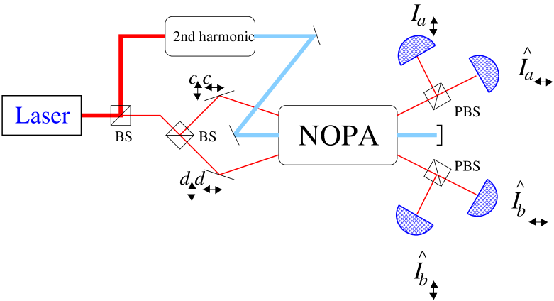
FIG. 1.: Experimental set-up for the tomographic test of Bell’s inequality. PBS and BS denote ‘polarizing beam splitter’ and ‘conventional beam splitter’ respectively. Input radiation modes $a_{\updownarrow}$, $b_{\leftrightarrow}$, $a_{\leftrightarrow}$ and $b_{\updownarrow}$ are in the vacuum state, while modes $c_{\updownarrow}$, $c_{\leftrightarrow}$, $d_{\updownarrow}$, $d_{\leftrightarrow}$ (at laser frequency $\omega_{0}$) are in a coherent state. At the output of the nondegenerate parametric amplifier (NOPA) the four photocurrents $\hat{I}$ at radiofrequency $\Omega$ are measured, yielding the value of quadratures of the field modes $a_{\updownarrow}$, $b_{\leftrightarrow}$, $a_{\leftrightarrow}$ and $b_{\updownarrow}$. The outcome quadratures are then used to reconstruct the probabilities of interest through quantum tomography.

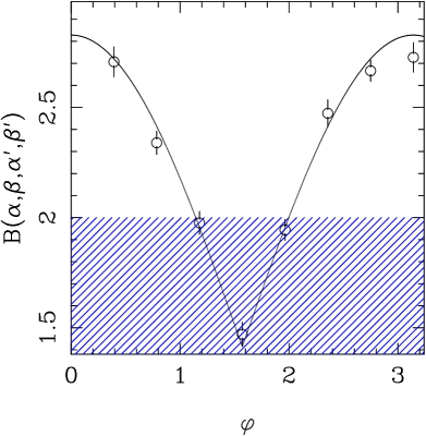
FIG. 2.: Plot of $B(\alpha,\beta,\alpha^{\prime},\beta^{\prime})$ vs the phase $\varphi$ in the state of Eq. (5) for a simulated experiment. The shaded area represents the classical region for $B$. The parameters of the simulation are: $\alpha=0;\ \beta=\frac{3}{8}\pi;\ \alpha^{\prime}=\frac{\pi}{4};\ \beta^{\prime}=\frac{\pi}{8}$; quantum efficiency $\eta=85\%$; average photon number per mode $N=0.5$. A total number of $10^{6}$ homodyne data (divided into $20$ statistical blocks) has been used.

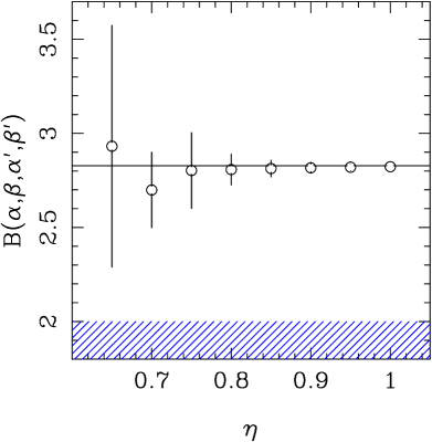
FIG. 3.: Plot of $B(\alpha,\beta,\alpha^{\prime},\beta^{\prime})$ vs the quantum efficiency of the detectors for a series of simulated experiments. The shaded area represents the classical region for $B$. The parameters of the simulations are: $\alpha=0;\ \beta=\frac{3}{8}\pi;\ \alpha^{\prime}=\frac{\pi}{4};\ \beta^{\prime}=\frac{\pi}{8}$; $\varphi=\pi$; $N=0.5$. A total number of $6\cdot 10^{7}$ homodyne data (in 20 statistical blocks) has been used for each simulation.

REFERENCES

- [1] A. Einstein, B. Podolsky, and N. Rosen, Phys. Rev. 47, 777 (1935).
- [2] N. Bohr, Phys. Rev. 48, 696 (1935).
- [3] J. S. Bell, Physics 1, 195 (1965).
- [4] J. F. Clauser, Phys. Rev. Lett. 36, 1223 (1976); A. Aspect, J. Dalibard, and G. Roger, Phys. Rev. Lett. 47, 460 (1981); A. J. Duncan, W. Perrie, H. J. Beyer, and H. Kleinpoppen, in Fundamental Processes in Atomic Collision Physics, Plenum, New York, 1985, pg. 555; Z. Y. Ou and L. Mandel, Phys. Rev. Lett. 61, 50 (1988); C. O. Alley and Y. H. Shih, Phys. Rev. Lett. 61, 2921 (1988); J. D. Franson, Phys. Rev. Lett. 62, 2200 (1989); K. Mattle, H. Weinfurter, P. G. Kwiat, and A. Zeilinger, Phys. Rev. Lett. 76, 4656 (1996).
- [5] J. F. Clauser, M. A. Horne, A. Shimony, and R. A. Holt, Phys. Rev. Lett. 23, 880 (1969); J. F. Clauser and M. A. Horne, Phys. Rev. D 10, 256 (1974); A. Garuccio and V. A. Rapisarda, Nuov. Cim. A 65, 269 (1981).
- [6] L. De Caro and A. Garuccio, Phys. Rev. A 54, 174 (1996).
- [7] D. T. Smithey, M. Beck, M. G. Raymer, and A. Faridani, Phys. Rev. Lett. 70, 1244 (1993).
- [8] G. Breitenbach, S. Schiller, and J. Mlynek, Nature 387, 471 (1997).
- [9] G. M. D’Ariano, Measuring quantum states, in Quantum Optics and the Spectroscopy of Solids, ed. by T. Hakioǧlu and A.S. Shumovsky, Kluwer Academic Publishers (1997), p. 175.
- [10] C. Kim and P. Kumar, Phys. Rev. Lett. 73, 1605 (1994).
- [11] G. M. D’Ariano, M. Vasilyev, and P. Kumar, Phys. Rev. A 58, 636 (1998).
- [12] D.Boschi, F. De Martini, and G. Di Giuseppe, in Quantum Interferometry, F. De Martini, G. Denardo and Y. Shih, Eds. (VCH, Wenheim 1996), p. 135.
- [13] G. M. D’Ariano, in Quantum Communication, Computing, and Measurement, ed. by O. Hirota, A. S. Holevo and C. M. Caves, Plenum Publishing (New York and London 1997), p. 253.
- [14] G. M. D’Ariano, U. Leonhardt, and H. Paul, Phys. Rev. A 52, R1801 (1995).
- [15] M. Vasilyev, S-K Choi, P. Kumar, and G. M. D’Ariano, Opt. Lett. 23, 1393 (1998).