LYCEN 9960a TUW-00-06 July 2000 Revised version

Mathematical surprises and Dirac’s formalism

in quantum mechanics

Dedicated to the memory of Tanguy Altherr (1963 - 1994)

François Gieres

Institut de Physique Nucléaire

Université Claude Bernard (Lyon 1)

43, boulevard du 11 novembre 1918

F - 69622 - Villeurbanne Cedex

Summary

By a series of simple examples, we illustrate how the lack of mathematical concern can readily lead to surprising mathematical contradictions in wave mechanics. The basic mathematical notions allowing for a precise formulation of the theory are then summarized and it is shown how they lead to an elucidation and deeper understanding of the aforementioned problems. After stressing the equivalence between wave mechanics and the other formulations of quantum mechanics, i.e. matrix mechanics and Dirac’s abstract Hilbert space formulation, we devote the second part of our paper to the latter approach: we discuss the problems and shortcomings of this formalism as well as those of the bra and ket notation introduced by Dirac in this context. In conclusion, we indicate how all of these problems can be solved or at least avoided.

Chapter 1 Introduction

Let us first provide an overview of the present article. The first part, covering section 2 and some complements gathered in the appendix, deals with mathematical surprises in quantum theory. It is accessible to all readers who have some basic notions in wave mechanics. The second part, consisting of section 4, deals with Dirac’s abstract Hilbert space approach and his bra and ket notation; it is devoted to a critical study of this formalism which has become the standard mathematical language of quantum physics during the last decades. Both parts are related by section 3 which discusses the equivalence between wave mechanics and the other formulations of quantum mechanics. As a consequence of this equivalence, the mentioned surprises also manifest themselves in these other formulations and in particular in Dirac’s abstract Hilbert space approach. In fact, one of the points we want to make in the second part, is that the lack of mathematical concern which is practically inherent in Dirac’s symbolic calculus, is a potential source for surprises and that it is harder, if not impossible, to elucidate unambiguously all mathematical contradictions within this formalism.

Let us now come to the motivation for our work and present in greater detail the outline of our discussion.

Mathematical surprises

In the formulation of physical theories, a lack of mathematical concern can often and readily lead to apparent contradictions which are sometimes quite astonishing. This is particularly true for quantum mechanics and we will illustrate this fact by a series of simple examples to be presented in section 2.1. In the literature, such contradictions appeared in the study of more complicated physical phenomena and they even brought into question certain physical effects like the Aharonov-Bohm effect [1]. These contradictions can only be discarded by appealing to a more careful mathematical formulation of the problems, a formulation which often provides a deeper physical understanding of the phenomena under investigation. Therefore, we strongly encourage the reader to look himself for a solution of all problems, eventually after a reading of section 2.2 in which we review the the mathematical formalism of wave mechanics. In fact, the latter review also mentions some mathematical tools which are not advocated in the majority of quantum mechanics textbooks, though they are well known in mathematical physics. The detailed solution of all of the raised problems is presented in the appendix. Altogether, this discussion provides an overview of the subtleties of the subject and of the tools for handling them in an efficient manner.

Dirac’s formalism

Since all of our examples of mathematical surprises are formulated in terms of the language of wave mechanics, one may wonder whether they are also present in other formulations of quantum theory. In this respect, we recall that there are essentially three different formulations or ‘representations’ that are used in quantum mechanics for the description of the states of a particle (or of a system of particles): wave mechanics, matrix mechanics and the invariant formalism. The first two rely on concrete Hilbert spaces, the last one on an abstract Hilbert space. In general, the latter formulation is presented using the bra and ket notation that Dirac developed from 1939 on, and that he introduced in the third edition of his celebrated textbook on the principles of quantum mechanics [2]. Let us briefly recall its main ingredients which will be discussed in the main body of the text:

$$\bullet \quad|\Psi\rangle\quad{\rm and}\quad\langle\Psi|$$

$$\bullet \quad A|\Psi\rangle\quad{\rm and}\quad\langle\Psi|A^{\displaystyle{\dagger}}$$

$$\bullet \quad\langle\Phi|A|\Psi\rangle$$

$$\bullet \quad\left\{|n\rangle\right\}_{n\in{\bf N}}\quad{\rm and}\quad\left\{|x\rangle\right\}_{x\in{\bf R}}$$

$$\bullet \quad|n_{1},n_{2},...\rangle\ \mbox{associated with a complete system of commuting observables}\ \left\{A_{1},A_{2},...\right\}.$$

This notation usually goes together with a specific interpretation of mathematical operations given by Dirac.

In this respect, it may be worthwhile to mention that Dirac’s classic monograph [2] (and thereby the majority of modern texts inspired by it) contains a fair number of statements which are ambiguous or incorrect from the mathematical point of view: these points have been raised and discussed by J.M.Jauch [3]. The state of affairs can be described as follows [4]: “Unfortunately, the elegance, outward clarity and strength of Dirac’s formalism are gained at the expense of introducing mathematical fictions. […] One has a formal ‘machinery’ whose significance is impenetrable, especially for the beginner, and whose problematics cannot be recognized by him.” Thus, the verdict of major mathematicians like J.Dieudonné is devastating [5]: “When one gets to the mathematical theories which are at the basis of quantum mechanics, one realizes that the attitude of certain physicists in the handling of these theories truly borders on the delirium. […] One has to wonder what remains in the mind of a student who has absorbed this unbelievable accumulation of nonsense, a real gibberish! It should be to believe that today’s physicists are only at ease in the vagueness, the obscure and the contradictory.” Certainly, we can blame many mathematicians for their intransigence and for their refusal to make the slightest effort to understand statements which lack rigor, even so their judgment should give us something to think about. By the present work, we hope to contribute in a constructive way to this reflection.

In section 3, we will define Dirac’s notation more precisely while recalling some mathematical facts and evoking the historical development of quantum mechanics. In section 4, we will successively discuss the following questions:

1. Is any of the three representations to be preferred to the other ones from the mathematical or practical point of view? In particular, we discuss the status of the invariant formalism to which the preference is given in the majority of recent textbooks.

2. What are the advantages, inconveniences and problems of Dirac’s notations and of their interpretation? (The computational rules inferred from these notations and their interpretation are usually applied in the framework of the invariant formalism and then define a symbolic calculus - as emphasized by Dirac himself in the introduction of his classic text [2].)

To anticipate our answer to these questions, we already indicate that we will reach the conclusion that the systematic application of the invariant formalism and the rigid use of Dirac’s notation - which are advocated in the majority of modern treatises of quantum mechanics - are neither to be recommended from a mathematical nor from a practical point of view. Compromises which retain the advantages of these formalisms while avoiding their shortcomings will be indicated. The conclusions which can be drawn for the practice and for the teaching of quantum theory are summarized in the final section (which also includes a short guide to the literature).

Chapter 2 Wave mechanics

2.1 Mathematical surprises in quantum mechanics

Examples which are simple from the mathematical point of view are to be followed by examples which are more sophisticated and more interesting from the physical point of view. All of them are formulated within the framework of wave mechanics and in terms of the standard mathematical language of quantum mechanics textbooks. The theory of wave mechanics being equivalent to the other formulations of quantum mechanics, the problems we mention are also present in the other formulations, though they may be less apparent there. The solution of all of the raised problems will be implicit in the subsequent section in which we review the mathematical formalism of wave mechanics. It is spelled out in detail in the appendix (but first think about it for yourself before looking it up!).

Example 1

For a particle in one dimension, the operators of momentum $P$ and position $Q$ satisfy Heisenberg’s canonical commutation relation

$$[P,Q]=\displaystyle{\hbar\over{\rm i}}\,{\bf 1}\ \ .$$ (2.1)

By taking the trace of this relation, one finds a vanishing result for the left-hand side, ${\rm Tr}\,[P,Q]=0$, whereas ${\rm Tr}\,(\displaystyle{\hbar\over{\rm i}}\,{\bf 1})\neq 0$. What is the conclusion?

Example 2

Consider wave functions $\varphi$ et $\psi$ which are square integrable on ${\bf R}$ and the momentum operator $P=\displaystyle{\hbar\over{\rm i}}\,\displaystyle{d\over dx}$. Integration by parts yields

$$\int_{-\infty}^{+\infty}dx\,\overline{\varphi(x)}\,(P\psi)(x)\ =\ \int_{-\infty}^{+\infty}dx\,\overline{(P\varphi)(x)}\,\psi(x)\,+\,\displaystyle{\hbar\over{\rm i}}\,\left[\left(\overline{\varphi}\,\psi\right)(x)\right]_{-\infty}^{+\infty}\ \ .$$

Since $\varphi$ and $\psi$ are square integrable, one usually concludes that these functions vanish for $x\to\pm\infty$. Thus, the last term in the previous equation vanishes, which implies that the operator $P$ is Hermitian.

However, the textbooks of mathematics tell us that square integrable functions do, in general, not admit a limit for $x\to\pm\infty$ and therefore they do not necessarily vanish at infinity. There are even functions which are continuous and square summable on ${\bf R}$ without being bounded at infinity [6]: an example of such a function is given by $f(x)=x^{2}\,{\rm exp}\,(-x^{8}\,{\rm sin}^{2}\,x)$, cf. figure 2.1 where the period of the function has been multiplied by a factor $20$ in order to increase the number of oscillations.

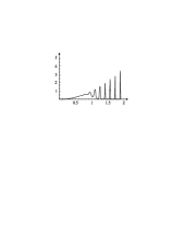
Figure 2.1: Graph of $f(x)=x^{2}\,{\rm exp}\,[-x^{8}\,{\rm sin}^{2}\,(20x)]$

We note that this example essentially amounts to a refinement of the following better known example [7] of a function which is continuous, positive and integrable on ${\bf R}$, though it does not tend to zero for $x\to\pm\infty$ (cf. figure 2.2): consider the “shrinking comb function” $f(x)=\sum_{n=2}^{\infty}f_{n}(x)$ where $f_{n}$ vanishes on ${\bf R}$, except on an interval of width $\displaystyle{2\over n^{2}}$ centered at $n$, where the graph of $f_{n}$ is a triangle, which is symmetrical with respect to $n$ and of height $1$.

Figure 2.2: Shrinking comb function

The area of this triangle being $\displaystyle{1\over n^{2}}$, we have

$$\int_{-\infty}^{+\infty}dx\,f(x)=\sum_{n=2}^{\infty}\,\displaystyle{1\over n^{2}}\,<\infty\ \ ,$$

but the function $f$ does not tend to zero for $x\to+\infty$.

Can one conclude that the operator $P$ is Hermitian in spite of these facts and if so, why?

Example 3

Consider the operators $P=\displaystyle{\hbar\over{\rm i}}\,\displaystyle{d\over dx}$ and ‘$Q=$ multiplication by $x$’ acting on wave functions depending on $x\in{\bf R}$. Since $P$ and $Q$ are Hermitian operators, the operator $A=PQ^{3}+Q^{3}P$ also has this property, because its adjoint is given by

$$A^{\displaystyle{\dagger}}=(PQ^{3}+Q^{3}P)^{\displaystyle{\dagger}}=Q^{3}P+PQ^{3}=A\ \ .$$

It follows that all eigenvalues of $A$ are real. Nevertheless, one easily verifies that

$$Af=\displaystyle{\hbar\over{\rm i}}\,f\qquad{\rm with}\quad f(x)\ =\left\{\begin{array}[]{ll}\displaystyle{1\over\sqrt{2}}\,|x|^{-3/2}\;{\rm exp}\,\left({-1\over 4x^{2}}\right)&{\rm for}\ x\neq 0\\ 0&{\rm for}\ x=0\ \ ,\end{array}\right.$$ (2.2)

which means that $A$ admits the complex eigenvalue $\hbar/{\rm i}$. Note that the function $f$ is infinitely differentiable on ${\bf R}$ and that it is square integrable, since

$$\int_{-\infty}^{\infty}dx\,|f(x)|^{2}\,=\,2\int_{0}^{\infty}dx\,|f(x)|^{2}\,=\,\int_{0}^{\infty}dx\,x^{-3}e^{-1/(2x^{2})}\,=\,\left[e^{-1/(2x^{2})}\right]_{0}^{\infty}\,=\,1\ \ .$$

Where is the error?

Example 4

Let us consider a particle confined to the interval $[0,1]$ and described by a wave function $\psi$ satisfying the boundary conditions $\psi(0)=0=\psi(1)$. Then the momentum operator $P=\displaystyle{\hbar\over{\rm i}}\,\displaystyle{d\over dx}$ is Hermitian, since the surface term appearing upon integration by parts vanishes:

$$\int_{0}^{1}dx\,\left(\overline{\varphi}\,(P\psi)-(\overline{P\varphi})\,\psi\right)(x)=\displaystyle{\hbar\over{\rm i}}\,\left[\left(\overline{\varphi}\,\psi\right)(x)\right]_{0}^{1}=0\ \ .$$ (2.3)

Since $P$ is Hermitian, its eigenvalues are real. In order to determine the latter, we note that the eigenvalue equation,

$$(P\psi_{p})(x)=p\,\psi_{p}(x)\qquad(p\in{\bf R}\ ,\ \psi_{p}\not\equiv 0)\ \ ,$$

is solved by $\psi_{p}(x)=c_{p}\,{\rm exp}\,(\displaystyle{{\rm i}\over\hbar}px)$ with $c_{p}\in{\bf C}-\{0\}$. The boundary condition $\psi_{p}(0)=0$ now implies $\psi_{p}\equiv 0$, therefore $P$ does not admit any eigenvalues. Nevertheless, the spectrum of $P$ is the entire complex plane [8] and $P$ does not represent an observable. How can one understand these results which seem astonishing?

Example 5

If one introduces polar coordinates in the plane or spherical coordinates in space, then the polar angle $\varphi$ and the component $L_{z}$ of angular momentum are canonically conjugate variables in classical mechanics. In quantum theory, the variable $\varphi$ becomes the operator of ‘multiplication of the wave function $\psi(\varphi)$ by $\varphi$’ and $L_{z}=\displaystyle{\hbar\over{\rm i}}\,\displaystyle{\partial\over\partial\varphi}$, which implies the commutation relation

$$[L_{z},\varphi]={\hbar\over{\rm i}}\,{\bf 1}\ \ .$$ (2.4)

These operators acting on periodic wave functions (i.e. $\psi(0)=\psi(2\pi)$) are Hermitian. Furthermore, $L_{z}$ admits a complete system of orthonormal eigenfunctions $\psi_{m}$,

$$L_{z}\psi_{m}=m\hbar\,\psi_{m}\qquad{\rm with}\quad\psi_{m}(\varphi)={1\over\sqrt{2\pi}}\;{\rm exp}\,({\rm i}m\varphi)\quad{\rm and}\quad m\in{\bf Z}\ \ .$$ (2.5)

(For the wave functions $\psi$, we only specify the dependence on the angular variable $\varphi$ and for the orthonormalisation, we refer to the standard scalar product for square integrable functions on the interval $[0,2\pi)$ :

$$\langle\psi_{1},\psi_{2}\rangle=\int_{0}^{2\pi}d\varphi\ \overline{\psi_{1}(\varphi)}\,\psi_{2}(\varphi)\ \ .)$$

By evaluating the average value of the operator $[L_{z},\varphi]$ in the state $\psi_{m}$ [9, 4] and by taking into account the fact that $L_{z}$ is Hermitian, one finds that

$${\hbar\over{\rm i}}\ =\ \langle\psi_{m},{\hbar\over{\rm i}}\,{\bf 1}\,\psi_{m}\rangle \stackrel{{\scriptstyle(\ref{lzp})}}{{=}} \langle\psi_{m},L_{z}\varphi\,\psi_{m}\rangle-\langle\psi_{m},\varphi L_{z}\,\psi_{m}\rangle$$

$$= \langle L_{z}^{\displaystyle{\dagger}}\,\psi_{m},\varphi\,\psi_{m}\rangle-m\hbar\,\langle\psi_{m},\varphi\,\psi_{m}\rangle$$

$$= (m\hbar-m\hbar)\,\langle\psi_{m},\varphi\,\psi_{m}\rangle\ =\ 0\ \ .$$

There must be a slight problem somewhere… (We note that similar problems appear for the phase and number operators which are of interest in quantum optics [9, 10].)

Example 6

Let us add a bit to the confusion of the previous example! In 1927, Pauli noted that the canonical commutation relation (2.1) implies Heisenberg’s uncertainty relation $\Delta P\cdot\Delta Q\geq\displaystyle{\hbar\over 2}$ by virtue of the Cauchy-Schwarz inequality. Since the commutation relation (2.4) has the same form as (2.1), one can derive, in the same way, the uncertainty relation

$$\Delta L_{z}\cdot\Delta\varphi\geq\displaystyle{\hbar\over 2}\ \ .$$ (2.7)

The following physical reasoning shows that this inequality cannot be correct [11, 9, 12]. One can always find a state for which $\Delta L_{z}<\hbar/4\pi$ and then the uncertainty for the angle $\varphi$ has to be larger than $2\pi$, which does not have any physical sense, since $\varphi$ takes values in the interval $[0,2\pi)$. How is it possible that relation (2.4) is correct, though the conclusion (2.7) is not?

By the way, this example shows that the uncertainty relation $\Delta A\cdot\Delta B\geq\displaystyle{1\over 2}\,|\,\langle[A,B]\rangle\,|$ for any two observables $A$ and $B$ (whose derivation can be found in most quantum mechanics texts) is not valid in such a generality.

Example 7

Let us consider a particle of mass $m$ in the infinite potential well

$$V(x)=\left\{\begin{array}[]{ll}0&{\rm if}\ \;|x|\leq a\quad\ (a>0)\\ \infty&{\rm otherwise}\ .\end{array}\right.$$

The Hamiltonian for the particle confined to the inside of the well is simply $H=\displaystyle{-\hbar^{2}\over 2m}\displaystyle{d^{2}\over dx^{2}}$. Let

$$\psi(x)=\displaystyle{\sqrt{15}\over 4a^{5/2}}\,(a^{2}-x^{2})\qquad{\rm for}\ |x|\leq a\quad(\,{\rm and}\ \,\psi(x)=0\ \,{\rm otherwise}\,)$$ (2.8)

be the normalized wave function of the particle at a given time. Since $H^{2}\psi=\displaystyle{\hbar^{4}\over 4m^{2}}\,\displaystyle{d^{4}\psi\over dx^{4}}=0$, the average value of the operator $H^{2}$ in the state $\psi$ vanishes :

$$\langle H^{2}\rangle_{\psi}=\langle\psi,H^{2}\psi\rangle=\int_{-a}^{+a}dx\;\overline{\psi(x)}\,(H^{2}\psi)(x)=0\ \ .$$ (2.9)

This average value can also be determined from the eigenvalues and eigenfunctions of $H$,

$$H\varphi_{n}=E_{n}\varphi_{n}\qquad{\rm with}\qquad E_{n}=\displaystyle{\pi^{2}\hbar^{2}\over 8ma^{2}}\,n^{2}\qquad(n=1,2,...)\ \ ,$$ (2.10)

by applying the formula

$$\langle H^{2}\rangle_{\psi}=\sum_{n=1}^{\infty}E_{n}^{2}\,p_{n}\qquad{\rm with}\ \,p_{n}=|\langle\varphi_{n},\psi\rangle|^{2}\ \ .$$ (2.11)

Proceeding in this way, one definitely does not find a vanishing result, because $E_{n}^{2}>0$ and $0\leq p_{n}\leq 1,\,\,\sum_{n=1}^{\infty}p_{n}=1$. In fact, the calculation yields $\langle H^{2}\rangle_{\psi}=\displaystyle{15\hbar^{4}\over 8m^{2}a^{4}}$. Which one of these two results is correct and where does the inconsistency come from? [4]

2.2 Clues to the understanding: the mathematical formalism

The problems and contradictions presented in the previous subsection can only be elucidated by resorting to a more precise mathematical formulation. Therefore, we now summarize the basic mathematical tools [6, 8][13]-[18] of wave mechanics in three subsections. The first two are sufficient for tackling the raised problems (and actually provide already some partial solutions); the last one has been added in order to round up the discussion and to provide a solid foundation for the subsequent section 4.

We consider the motion of a particle on a straight line parametrized by $x\in{\bf R}$. The generalization to a bounded interval, to three dimensions, to the spin or to a system of particles does not present any problems.

2.2.1 The space of states

Born’s probabilistic interpretation of the wave function $\psi$ requires that

$$\int_{{\bf R}}|\psi(x,t)|^{2}dx=1\qquad{\rm for\ \;all}\ \ t\in{\bf R}\ \ .$$

Thus, the wave function which depends continuously on the time parameter $t$, must be square integrable with respect to the space variable $x$:

$$\psi : {\bf R}\times{\bf R}\ \to\ {\bf C}$$

$$\ (x,t)\ \ \,\mapsto\ \psi(x,t)\equiv\psi_{t}(x)\qquad{\rm with}\quad\psi_{t}\in L^{2}({\bf R},dx)\ \ .$$

Here, ${L^{2}({{\bf R}},dx)}$ is the space of square integrable functions,

$${L^{2}({{\bf R}},dx)}=\{f:{\bf R}\to{\bf C}\ \mid\ \int_{{\bf R}}dx\,|f(x)|^{2}<\infty\}\ \ ,$$

with the scalar product

$$\langle f,g\rangle_{L^{2}}=\int_{{\bf R}}dx\;\overline{f(x)}\,g(x)\qquad\mbox{for}\ \;f,g\in{L^{2}({{\bf R}},dx)}\ \ .$$ (2.12)

For later reference, we recall that this space is related by the Fourier transformation to the Hilbert space $L^{2}({\bf R},dp)$ of wave functions depending on the momentum $p$ :

$${\cal F}\ : {L^{2}({{\bf R}},dx)} \longrightarrow\ \ L^{2}({{\bf R}},dp)$$

$$f \longmapsto\ \ {\cal F}f\quad{\rm with}\ \;\left({\cal F}f\right)(p)={1\over\sqrt{2\pi\hbar}}\int_{{\bf R}}dx\,f(x)\,{\rm exp}(-{{\rm i}\over\hbar}px)\ \ .$$

2.2.2 Operators

In this section, we will properly define the notion of an operator and its adjoint (the Hermitian conjugate operator), as well as Hermitian operators and self-adjoint operators (i.e. physical observables). Furthermore, we will indicate how the properties of the spectrum of a given operator are intimately connected with the mathematical characteristics of this operator and of its eigenfunctions. We strongly encourage the reader who is not familiar with the definitions and results spelled out at the beginning of this subsection to pursue the reading with the illustrations that follow.

The following considerations (i.e. sections 2.2.2 and 2.2.3) do not only apply to the concrete Hilbert space ${L^{2}({{\bf R}},dx)}$ of wave mechanics, but to any Hilbert space ${\cal H}$ that is isomorphic to it, i.e. any complex Hilbert space which admits a countably infinite basis; therefore, we will refer to a general Hilbert space ${\cal H}$ of this type and only specialize to the concrete realizations ${L^{2}({{\bf R}},dx)}$ or $L^{2}([0,1],dx)$ in the examples.

Just as a function $f:{\bf R}\to{\bf R}$ has a domain of definition ${\cal D}(f)\subset{\bf R}$, a Hilbert space operator $A:{\cal H}\to{\cal H}$ admits such a domain:

Definition 1

An operator on the Hilbert space ${\cal H}$ is a linear map

$$A\ : {\cal D}(A) \longrightarrow\ \ {\cal H}$$

$$\psi \longmapsto\ \ A\psi\ \ ,$$

where ${\cal D}(A)$ represents a dense linear subspace of ${\cal H}$. This subspace is called the domain of definition of $A$ or, for short, the domain of $A$. (Thus, strictly speaking, a Hilbert space operator is a pair $(A,{\cal D}(A)$) consisting of a prescription of operation on the Hilbert space, together with a Hilbert space subset on which this operation is defined.)

If $B$ denotes another operator on ${\cal H}$ $($with domain ${\cal D}(B))$, then the operator $A$ is said to be equal to the operator $B$ if both the prescription of operation and the domain of definition coincide, i.e. if

$$A\varphi=B\varphi\qquad\mbox{for all}\ \varphi\in{\cal D}(A)={\cal D}(B)\ \ .$$

In this case, one writes $A=B$.

We note that, in the mathematical literature, the definition of an operator is usually phrased in more general terms by dropping the assumptions that ${\cal D}(A)$ is dense and that the map $A$ is linear; however, these generalizations scarcely occur in quantum mechanics and therefore we will not consider them here.

As emphasized in the previous definition, an operator is not simply a formal operating prescription and two operators which act in the same way are to be considered as different if they are not defined on the same subspace of Hilbert space. A typical example for the latter situation is given by a physical problem on a compact or semi-infinite interval: the domain of definition of operators then includes, in general, some boundary conditions whose choice depends on the experimental set-up which is being considered. Clearly, two non equivalent experimental set-ups for the measurement of a given physical observable generally lead to different experimental results: thus, it is important to consider as different two Hilbert space operators which act in the same way, but admit different domains of definition. Actually, most of the contradictions derived in section 2 can be traced back to the fact that the domains of definition of the operators under consideration have been ignored!

By way of example, let us first consider three different operators on the Hilbert space ${\cal H}={L^{2}({{\bf R}},dx)}$ and then another one on $L^{2}([0,1])$.

1.a) The position operator $Q$ for a particle on the real line is the operator ‘multiplication by $x$’ on ${L^{2}({{\bf R}},dx)}$:

$$\left(Q\psi\right)(x)=x\,\psi(x)\quad\mbox{for all $x\in{\bf R}$}\ \ .$$ (2.15)

The maximal domain of definition for $Q$ is the one which ensures that the function $Q\psi$ exists and that it still belongs to the Hilbert space :

$${\cal D}_{\rm max}(Q) = \{\psi\in{\cal H}\ |\ Q\psi\in{\cal H}\}$$ (2.16)

$$= \{\psi\in{L^{2}({{\bf R}},dx)}\ |\ \|Q\psi\|^{2}\equiv\int_{{\bf R}}dx\,x^{2}|\psi(x)|^{2}<\infty\}\ \ .$$

Obviously, this represents a proper subspace of ${L^{2}({{\bf R}},dx)}$ and it can be shown that it is a dense subspace [8, 14].

1.b) Analogously, the maximal domain of definition of the momentum operator $P=\displaystyle{\hbar\over{\rm i}}\,\displaystyle{d\over dx}$ on the Hilbert space ${L^{2}({{\bf R}},dx)}$ is

$${\cal D}_{\rm max}(P)=\{\psi\in{L^{2}({{\bf R}},dx)}\,|\,\psi^{\prime}\in{L^{2}({{\bf R}},dx)}\}\ \ .$$

1.c) For certain considerations it is convenient to have at one’s disposal a domain of definition that is left invariant by the operator (rather than a maximally defined operator). For the operator $Q$, such a domain is given by the Schwartz space ${\cal S}({\bf R})$ of rapidly decreasing functions. Let us recall that a function $f:{\bf R}\to{\bf C}$ belongs to ${\cal S}({\bf R})$ if it is differentiable an infinite number of times and if this function, as well as all of its derivatives, decreases more rapidly at infinity than the inverse of any polynomial). This implies that ${\cal S}({\bf R})\subset{\cal D}_{\rm max}(Q)$ and

$$Q\ :\ {\cal S}({\bf R})\longrightarrow{\cal S}({\bf R})\ \ .$$ (2.17)

The Schwartz space also represents an invariant domain of definition for the momentum operator $P=\displaystyle{\hbar\over{\rm i}}\,\displaystyle{d\over dx}$ on ${L^{2}({{\bf R}},dx)}$, i.e. $P\,:\,{\cal S}({\bf R})\rightarrow{\cal S}({\bf R})$.

According to the definition given above, the operators $P$ and $Q$ introduced in the last example are different from $P$ and $Q$ as defined in the preceding two examples, respectively; however, in the present case where we have an infinite interval, this difference is rather a mathematical one since physical measurements do not allow us to make a distinction between the different domains.

2. Let us also give an example concerning a particle which is confined to a compact interval e.g. $[0,1]$. In this case, the wave function generally satisfies some boundary conditions which have to be taken into account by means of the domains of the operators under investigation. For instance, let us consider example 4 of section 2, i.e. the momentum operator $P$ on ${\cal H}=L^{2}([0,1],dx)$ with the usual boundary conditions of an infinite potential well: the domain of definition of $P$ then reads

$${\cal D}(P)=\{\psi\in{\cal H}\,|\,\psi^{\prime}\in{\cal H}\ {\rm and}\ \psi(0)=0=\psi(1)\}\ \ .$$ (2.18)

Shortly, we will come to the mathematical and physical properties of this quantum mechanical operator.

The specification of the domain plays a crucial role when introducing the adjoint $A^{\displaystyle{\dagger}}$ of a Hilbert space operator $A$:

Definition 2

For an operator $A$ on ${\cal H}$, the domain of $A^{\displaystyle{\dagger}}$ is defined by

$${\cal D}(A^{\displaystyle{\dagger}}) = \{\varphi\in{\cal H}\,|\,\exists\,\tilde{\varphi}\in{\cal H}\ \ \mbox{such that}$$

$$\qquad\qquad\qquad\qquad\quad\left\langle\varphi,A\psi\right\rangle=\langle\,\tilde{\varphi}\,,\,\psi\,\rangle\ \mbox{for all}\ \psi\in{\cal D}(A)\}\ \ .$$

(Here, the vector $\tilde{\varphi}$ depends on both $A$ and $\varphi$.) For $\varphi\in{\cal D}(A^{\displaystyle{\dagger}})$, one defines $A^{\displaystyle{\dagger}}\varphi=\tilde{\varphi}$, i.e.

$$\langle\varphi,A\psi\rangle=\langle A^{\displaystyle{\dagger}}\varphi,\psi\rangle\qquad\mbox{for all}\ \psi\in{\cal D}(A)\ \ .$$ (2.19)

By way of example, we again consider the Hilbert space ${\cal H}=L^{2}([0,1],dx)$ and the momentum operator $P$ with the domain (2.18). According to the previous definition, the domain of $P^{\displaystyle{\dagger}}$ is given by

$${\cal D}(P^{\displaystyle{\dagger}})=\{\varphi\in{\cal H}\,|\,\exists\,\tilde{\varphi}\in{\cal H}\ \mbox{such that}\ \langle\varphi,P\psi\rangle=\langle\tilde{\varphi},\psi\rangle\ \mbox{for all}\ \psi\in{\cal D}(P)\}$$

and the operating prescription for $P^{\displaystyle{\dagger}}$ is determined by the relation

$$\langle\varphi,P\psi\rangle=\langle P^{\displaystyle{\dagger}}\varphi,\psi\rangle\qquad\mbox{for all}\ \psi\in{\cal D}(P)\ \ .$$ (2.20)

The integration by parts (2.3) or, more precisely,

$$\int_{0}^{1}\!dx\,(\overline{\varphi}\,P\psi-\left(\overline{\displaystyle{\hbar\over{\rm i}}\,\displaystyle{d\varphi\over dx}}\right)\psi)(x) = \displaystyle{\hbar\over{\rm i}}\left[\overline{\varphi(1)}\psi(1)-\overline{\varphi(0)}\psi(0)\right]$$

$$= 0\qquad\mbox{for all}\ \,\psi\in{\cal D}(P)$$

shows that the boundary conditions satisfied by $\psi\in{\cal D}(P)$ are already sufficient for annihilating the surface term and it shows that $P^{\displaystyle{\dagger}}$ acts in the same way as $P$. Hence,

$$P^{\displaystyle{\dagger}}=\displaystyle{\hbar\over{\rm i}}\,\displaystyle{d\over dx}\quad,\quad{\cal D}(P^{\displaystyle{\dagger}})=\{\varphi\in{\cal H}\,|\,\varphi^{\prime}\in{\cal H}\}\ \ .$$ (2.21)

Thus, the domain of definition of $P^{\displaystyle{\dagger}}$ is larger than the one of $P$: ${\cal D}(P)\subset{\cal D}(P^{\displaystyle{\dagger}})$.

In quantum theory, physical observables are described by Hilbert space operators which have the property of being self-adjoint. Although many physics textbooks use this term as a synonym for Hermitian, there exists a subtle difference between these two properties for operators acting on infinite dimensional Hilbert spaces: as we will illustrate in the sequel, this difference is important for quantum physics.

Definition 3

The operator $A$ on ${\cal H}$ is Hermitian if

$$\langle\varphi,A\psi\rangle=\langle A\varphi,\psi\rangle\qquad\mbox{for all}\ \varphi,\psi\in{\cal D}(A)$$ (2.22)

i.e.

$$A^{\displaystyle{\dagger}}\varphi=A\varphi\qquad\mbox{for all}\ \varphi\in{\cal D}(A)\ \ .$$

(In other words, the operator $A$ is Hermitian if $A^{\displaystyle{\dagger}}$ acts in the same way as $A$ on all vectors belonging to ${\cal D}(A)$, though $A^{\displaystyle{\dagger}}$ may actually be defined on a larger subspace than ${\cal D}(A)$.)

An operator $A$ on ${\cal H}$ is self-adjoint if the operators $A$ and $A^{\displaystyle{\dagger}}$ coincide ($A=A^{\displaystyle{\dagger}}$), i.e. explicitly

$${\cal D}(A)={\cal D}(A^{\displaystyle{\dagger}})\qquad and\qquad A^{\displaystyle{\dagger}}\varphi=A\varphi\quad\mbox{for all}\ \varphi\in{\cal D}(A)\ \ .$$ (2.23)

Thus, any self-adjoint operator is Hermitian, but an Hermitian operator is not necessarily self-adjoint. Our previous example provides an illustration for the latter fact. We found that $P$ and $P^{\displaystyle{\dagger}}$ act in the same way, though the domain of definition of $P^{\displaystyle{\dagger}}$ (as given by equation (2.21)) is strictly larger than the one of $P$ (as given by equation (2.18)): ${\cal D}(P)\subset{\cal D}(P^{\displaystyle{\dagger}})$, but ${\cal D}(P)\neq{\cal D}(P^{\displaystyle{\dagger}})$. From these facts, we conclude that $P$ is Hermitian, but not self-adjoint: $P\neq P^{\displaystyle{\dagger}}$.

One may wonder whether it is possible to characterize in another way the little “extra” that a Hermitian operator is lacking in order to be self-adjoint. This missing item is exhibited by the following result which is proven in mathematical textbooks. If the Hilbert space operator $A$ is self-adjoint, then its spectrum is real [6, 8][13]-[18] and the eigenvectors associated to different eigenvalues are mutually orthogonal; moreover, the eigenvectors together with the generalized eigenvectors yield a complete system of (generalized) vectors of the Hilbert space [19, 20, 8]. These results do not hold for operators which are only Hermitian. As we saw in section 2.1, this fact is confirmed by our previous example: the Hermitian operator $P$ does not admit any proper or generalized eigenfunctions and therefore it is not self-adjoint (as we already deduced by referring directly to the definition of self-adjointness).

Concerning these aspects, we recall that the existence of a complete system of (generalized) eigenfunctions is fundamental for the physical interpretation of observables. It motivates the mathematical definition of an observable which is usually given in textbooks on quantum mechanics: an observable is defined as a “Hermitian operator whose orthonormalized eigenvectors define a basis of Hilbert space” [21]. The shortcomings of this approach (as opposed to the identification of observables with self-adjoint operators) will be discussed in section 4. Here, we only note the following. For a given Hilbert space operator, it is usually easy to check whether it is Hermitian (e.g. by performing some integration by parts). And for a Hermitian operator, there exist simple criteria for self-adjointness: the standard one will be stated and applied in the appendix.

Finally, we come to the spectrum of operators for which we limit ourselves to the general ideas. By definition, the spectrum of a self-adjoint operator $A$ on the Hilbert space ${\cal H}$ is the union of two sets of real numbers,

1. the so-called discrete or point spectrum, i.e. the set of eigenvalues of $A$ (that is eigenvalues for which the eigenvectors belong to the domain of definition of $A$).

2. the so-called continuous spectrum, i.e. the set of generalized eigenvalues of $A$ (that is eigenvalues for which “the eigenvectors do not belong to the Hilbert space ${\cal H}$”).

These notions will be made more precise and illustrated in the next subsection as well as in the appendix. From the physical point of view, the spectral values of an observable (given by a self-adjoint operator) are the possible results that one can find upon measuring this physical quantity. The following two examples are familiar from physics.

1. For a particle moving on a line, the observables of position and momentum can both take any real value. Thus, the corresponding operators have a purely continuous and unbounded spectrum: ${\rm Sp}\,Q={\bf R}$ and ${\rm Sp}\,P={\bf R}$. A rigorous proof of this result will be given shortly (equations (2.26)-(2.2.3) below).

2. For a particle confined to the unit interval and subject to periodic boundary conditions, we have wave functions belonging to the Hilbert space $L^{2}([0,1],dx)$ and satisfying the boundary conditions $\psi(0)=\psi(1)$. In this case, the position operator admits a continuous and bounded spectrum given by the interval $[0,1]$. The spectrum of the momentum operator is discrete and unbounded, which means that the momentum can only take certain discrete, though arbitrary large values.

In order to avoid misunderstandings, we should emphasize that the definitions given in physics and mathematics textbooks, respectively, for the spectrum of an operator acting on an infinite dimensional Hilbert space, do not completely coincide. In fact, from a mathematical point of view it is not natural to simply define the spectrum of a generic Hilbert space operator as the set of its proper and generalized eigenvalues (e.g. see references [3] and [8]): by definition, it contains a third part, the so-called residual spectrum. The latter is empty for self-adjoint operators and therefore we did not mention it above. However, we will see in the appendix that the residual spectrum is not empty for operators which are only Hermitian; we will illustrate its usefulness for deciding whether a given Hermitian operator can possibly be modified so as to become self-adjoint (i.e. precisely the criteria for self-adjointness of a Hermitian operator that we already evoked).

Before concluding our overview of Hilbert space operators, we note that all definitions given in this subsection also hold if the complex Hilbert space ${\cal H}$ is of finite dimension $n$, i.e. ${\cal H}\simeq{\bf C}^{n}$. In this case (which is of physical interest for the spin of a particle or for a quantum mechanical two-level system), the previous results simplify greatly:

- any operator $A$ on ${\cal H}$ (which may now be expressed in terms of a complex $n\times n$ matrix) and its adjoint (the Hermitian conjugate matrix) are defined on the whole Hilbert space, i.e. ${\cal D}(A)={\cal H}$

- Hermitian and self-adjoint are now synonymous

- the spectrum of $A$ is simply the set of all its eigenvalues, i.e. we have a purely discrete spectrum.

Yet, it is plausible that the passage to infinite dimensions, i.e. the addition of an infinite number of orthogonal directions to ${\bf C}^{n}$ opens up new possibilities! As S.MacLane put it: “Gentlemen: there’s lots of room left in Hilbert space.” [14]

2.2.3 Observables and generalized eigenfunctions

When introducing the observables of position and momentum for a particle on the real line, we already noticed that they are not defined on the entire Hilbert space, but only on a proper subspace of it. In this section, we will point out and discuss some generic features of quantum mechanical observables.

Two technical complications appear in the study of an observable $A$ in quantum mechanics:

(i) If the spectrum of $A$ is not bounded, then the domain of definition of $A$ cannot be all of ${\cal H}$.

(ii) If the spectrum of $A$ contains a continuous part, then the corresponding eigenvectors do not belong to ${\cal H}$, but rather to a larger space.

Let us discuss these two problems in turn before concluding with some related remarks.

(i) Unbounded operators

The simplest class of operators is the one of bounded operators, i.e. for every vector $\psi\in{\cal D}(A)$, one has

$$\|A\psi\|\leq c\,\|\psi\|\qquad\mbox{where $c\geq 0$ is a constant}\ \ .$$ (2.24)

This condition amounts to say that the spectrum of $A$ is bounded. Bounded operators can always be defined on the entire Hilbert space, i.e. ${\cal D}(A)={\cal H}$. An important example is the one of an unitary operator $U:{\cal H}\to{\cal H}$ ; such an operator is bounded, because it is norm-preserving (i.e. $\|U\psi\|=\|\psi\|$ for all $\psi\in{\cal H}$) and therefore condition (2.24) is satisfied. (The spectrum of $U$ lies on the unit circle of the complex plane and therefore it is bounded. For instance, the spectrum of the Fourier transform operator ${\cal F}$ defined by (2.2.1) is the discrete set $\{\pm 1,\pm{\rm i}\}$ [13, 16].)

A large part of the mathematical subtleties of quantum mechanics originates from the following result [8, 14].

Theorem 1 (Hellinger-Toeplitz)

Let $A$ be an operator on ${\cal H}$ which is everywhere defined and which satisfies the Hermiticity condition

$$\langle\varphi,A\psi\rangle=\langle A\varphi,\psi\rangle$$ (2.25)

for all vectors $\varphi,\psi\in{\cal H}$. Then $A$ is bounded.

In quantum theory, one often deals with operators, like those associated to the position, momentum or energy, which fulfill the Hermiticity condition (2.25) on their domain of definition, but for which the spectrum is not bounded. (In fact, the basic structural relation of quantum mechanics, i.e. the canonical commutation relation, even imposes that some of the fundamental operators, which are involved in it, are unbounded - see appendix.) The preceding theorem indicates that it is not possible to define these Hermitian operators on the entire Hilbert space ${\cal H}$ and that their domain of definition necessarily represents a proper subspace of ${\cal H}$. Among all the choices of subspace which are possible from the mathematical point of view, certain ones are usually privileged by physical considerations (boundary conditions, …) [22, 14, 8, 23, 24].

By way of example, we consider the position operator $Q$ defined on the Schwartz space ${\cal S}({\bf R})$, see eqs.(2.15)(2.17). This operator is Hermitian since all vectors $\varphi,\psi\in{\cal S}({\bf R})$ satisfy

$$\langle\varphi,Q\psi\rangle=\int_{{\bf R}}dx\,\overline{\varphi}\,x\psi=\int_{{\bf R}}dx\,\overline{x\varphi}\,\psi=\langle Q\varphi,\psi\rangle\ \ .$$

As we are going to prove shortly, the spectrum of this operator is the entire real axis (reflecting the fact that $Q$ is not bounded). For this specific operator, we already noticed explicitly that there is no way to define $Q$ on all vectors of Hilbert space: at best, it can be defined on its maximal domain (2.16) which represents a nontrivial subspace of Hilbert space.

(ii) Generalized eigenfunctions (Gelfand triplets)

The position operator Q defined on ${\cal S}({\bf R})$ also illustrates the fact that the eigenvectors associated to the continuous spectrum of a self-adjoint operator do not belong to the Hilbert space. In fact, the eigenfunction $\psi_{x_{0}}$ associated to the eigenvalue $x_{0}\in{\bf R}$ is defined by the relation

$$\left(Q\psi_{x_{0}}\right)(x)=x_{0}\,\psi_{x_{0}}(x)\qquad(x_{0}\in{\bf R}\ ,\ \psi_{x_{0}}\in{\cal S}({\bf R})\ ,\ \psi_{x_{0}}\not\equiv 0)$$ (2.26)

or else, following (2.15), by

$$(x-x_{0})\,\psi_{x_{0}}(x)=0\quad\mbox{for all $x\in{\bf R}$}\ \ .$$

This condition implies $\psi_{x_{0}}(x)=0$ for $x\neq x_{0}$. Consequently, the function $\psi_{x_{0}}$ vanishes almost everywhere and thus represents the null vector of ${L^{2}({{\bf R}},dx)}$ [8, 13, 14]. Hence, the operator $Q$ does not admit any eigenvalue: its discrete spectrum is empty.

We note that the situation is the same for the operator $P$ defined on ${\cal S}({\bf R})$ which is also essentially self-adjoint: the eigenvalue equation

$$\left(P\psi_{p}\right)(x)=p\,\psi_{p}(x)\qquad(p\in{\bf R}\ ,\ \psi_{p}\in{\cal S}({\bf R})\ ,\ \psi_{p}\not\equiv 0),\ \ ,$$

is solved by $\psi_{p}(x)=1/\sqrt{2\pi\hbar}\ {\rm exp}({\rm i}px/\hbar)$, but $\psi_{p}\not\in{\cal S}({\bf R})$. Thus $P$ does not admit any eigenvalue.

On the other hand, the eigenvalue equations for $Q$ and $P$ admit weak (distributional) solutions. For instance, Dirac’s generalized function (distribution) with support in $x_{0}$, i.e. $\delta_{x_{0}}(x)\equiv\delta(x-x_{0})$, is a weak solution of the eigenvalue equation (2.26): in order to check that $x\,\delta_{x_{0}}(x)=x_{0}\,\delta_{x_{0}}(x)$ in the sense of distributions, we have to smear out this relation with a test function $\varphi\in{\cal S}({\bf R})$:

$$\int_{{\bf R}}dx\,x\,\delta_{x_{0}}(x)\,\varphi(x)=x_{0}\,\varphi(x_{0})=\int_{{\bf R}}dx\,x_{0}\,\delta_{x_{0}}(x)\,\varphi(x)\ \ .$$ (2.27)

Dirac’s generalized function and the generalized function $x\delta_{x_{0}}$ do not belong to the domain of definition ${\cal S}({\bf R})$ of $Q$, rather they belong to its dual space

$${\cal S}^{\prime}({\bf R})=\{\omega:{\cal S}({\bf R})\to{\bf C}\ \mbox{linear and continuous}\}\ \ ,$$

i.e. the space of tempered distributions on ${\bf R}$ [14, 8, 15, 25, 19]. They are defined in an abstract and rigorous manner by

$$\delta_{x_{0}}\ : {\cal S}({\bf R}) \longrightarrow\ \ {\bf C}$$

$$\varphi \longmapsto\ \ \delta_{x_{0}}(\varphi)=\varphi(x_{0})$$

and

$$x\,\delta_{x_{0}}\ : {\cal S}({\bf R}) \longrightarrow\ \ {\bf C}$$

$$\varphi \longmapsto\ \ \left(x\,\delta_{x_{0}}\right)(\varphi)=\delta_{x_{0}}(x\varphi)\stackrel{{\scriptstyle(\ref{xd})}}{{=}}x_{0}\,\varphi(x_{0})\ \ .$$

With these definitions, the formal writing (2.27) takes the precise form

$$\left(x\,\delta_{x_{0}}\right)(\varphi)=\left(x_{0}\,\delta_{x_{0}}\right)(\varphi)\qquad\mbox{for all}\ \ \varphi\in{\cal S}({\bf R})\ \ .$$

Thus, the eigenvalue equation $Q\psi_{x_{0}}=x_{0}\,\psi_{x_{0}}$ admits a distributional solution $\psi_{x_{0}}$ for every value $x_{0}\in{\bf R}$. Since the spectrum of the (essentially self-adjoint) operator $Q$ is the set of all real numbers for which the eigenvalue equation admits as solution either a function $\psi\in{\cal D}(Q)={\cal S}({\bf R})$ (discrete spectrum) or a generalized function $\psi\in{\cal S}^{\prime}({\bf R})$ (continuous spectrum), we can conclude that ${\rm Sp}\,Q={\bf R}$ and that the spectrum of $Q$ is purely continuous.

Analogously, the function $\psi_{p}(x)=1/\sqrt{2\pi\hbar}\ {\rm exp}({\rm i}px/\hbar)$ defines a distribution $l_{p}$ according to

$$l_{p}\ : {\cal S}({\bf R}) \longrightarrow\ \ {\bf C}$$

$$\varphi \longmapsto\ \ l_{p}(\varphi)=\int_{{\bf R}}dx\,\overline{\psi_{p}(x)}\,\varphi(x)\stackrel{{\scriptstyle(\ref{f})}}{{=}}({\cal F}\varphi)(p)\ \ ,$$

where ${\cal F}\varphi$ denotes the Fourier transform (2.2.1). The distribution $l_{p}$ represents a solution of the eigenvalue equation $Pl_{p}=p\,l_{p}$ since the calculational rules for distributions and Fourier transforms [8, 19] and the definition (2.2.3) imply that

$$\left(Pl_{p}\right)(\varphi)=\left(\displaystyle{\hbar\over{\rm i}}\,\displaystyle{dl_{p}\over dx}\right)(\varphi)=l_{p}\left(\displaystyle{\hbar\over{\rm i}}\,\displaystyle{d\varphi\over dx}\right)\stackrel{{\scriptstyle(\ref{dis})}}{{=}}({\cal F}\left(\displaystyle{\hbar\over{\rm i}}\,\displaystyle{d\varphi\over dx}\right))(p)=p\,({\cal F}\varphi)(p)\stackrel{{\scriptstyle(\ref{dis})}}{{=}}p\,l_{p}(\varphi)\ \ .$$

It follows that ${\rm Sp}\,P={\bf R}$ (purely continuous spectrum).

The eigenvalue problem for the operators $P$ and $Q$ which admit a continuous spectrum thus leads us to consider the following Gelfand triplet (“rigged or equipped Hilbert space”)

$$\framebox{\mbox{$\ {\cal S}({\bf R})\subset{L^{2}({{\bf R}},dx)}\subset{\cal S}^{\prime}({\bf R})\ $}}\ \ .$$ (2.30)

Here, ${\cal S}({\bf R})$ is a dense subspace of ${L^{2}({{\bf R}},dx)}$ [14] and every function $\psi\in{L^{2}({{\bf R}},dx)}$ defines a distribution $\omega_{\psi}\in{\cal S}^{\prime}({\bf R})$ according to

$$\omega_{\psi}\ : {\cal S}({\bf R}) \longrightarrow\ \ {\bf C}$$ (2.31)

$$\varphi \longmapsto\ \ \omega_{\psi}(\varphi)=\int_{{\bf R}}dx\,\overline{\psi(x)}\varphi(x)\ \ .$$

However ${\cal S}^{\prime}({\bf R})$ also contains distributions like Dirac’s distribution $\delta_{x_{0}}$ or the distribution $l_{p}$ which cannot be represented by means of a function $\psi\in{L^{2}({{\bf R}},dx)}$ according to (2.31). The procedure of smearing out with a test function $\varphi\in{\cal S}({\bf R})$ corresponds to the formation of wave packets and the theory of distributions gives a quite precise meaning to this procedure as well as to the generalized functions that it involves.

The abstract definition of the triplet (2.30) can be made more precise (e.g. specification of the topology on ${\cal S}({\bf R})$,…) and, furthermore, ${\cal S}({\bf R})$ can be generalized to other subspaces of ${L^{2}({{\bf R}},dx)}$ (associated to $Q$ or to other operators defined on ${L^{2}({{\bf R}},dx)}$). Up to these details (which are important and which have to be taken into account in the study of a given Hilbert space operator), we can say that

the triplet (2.30) describes in an exact and simple manner the mathematical nature of all kets and bras used in quantum mechanics.

In fact, according to the Riesz lemma (which is recalled in section 3.1.1 below), the Hilbert space ${L^{2}({{\bf R}},dx)}$ is isometric to its dual: thus, to each ket belonging to ${L^{2}({{\bf R}},dx)}$, there corresponds a bra given by an element of ${L^{2}({{\bf R}},dx)}$, and conversely. Moreover, a ket belonging to the subspace ${\cal S}({\bf R})$ always defines a bra belonging to ${\cal S}^{\prime}({\bf R})$ by virtue of definition (2.31). But there exist elements of ${\cal S}^{\prime}({\bf R})$, the generalized bras, to which one cannot associate a ket belonging to ${\cal S}({\bf R})$ or ${L^{2}({{\bf R}},dx)}$. We note that the transparency of this mathematical result is lost if one proceeds as one usually does in quantum mechanics, namely if one describes the action of a distribution on a test function $\varphi$ in a purely formal manner as a scalar product between $\varphi\in{\cal S}({\bf R})\subset{L^{2}({{\bf R}},dx)}$ and a function which does not belong to ${L^{2}({{\bf R}},dx)}$:

$$l_{p}(\varphi)\! \!=\! \!\left\langle\psi_{p},\varphi\right\rangle_{L^{2}}\equiv\int_{{\bf R}}dx\,\overline{\psi_{p}(x)}\,\varphi(x)\qquad(\,\mbox{ignoring that}\ \psi_{p}\not\in{L^{2}({{\bf R}},dx)}\,)$$

$$\delta_{x_{0}}(\varphi)\! \!=\! \!\left\langle\delta_{x_{0}},\varphi\right\rangle_{L^{2}}\equiv\int_{{\bf R}}dx\,\overline{\delta_{x_{0}}(x)}\,\varphi(x)\quad\ \ (\,\mbox{ignoring that}\ \delta_{x_{0}}\not\in{L^{2}({{\bf R}},dx)}\,).$$ (2.32)

Quite generally, let us consider a self-adjoint operator $A$ on the Hilbert space ${\cal H}$. The eigenfunctions associated to elements of the continuous spectrum of $A$ do not belong to the Hilbert space ${\cal H}$: one has to equip ${\cal H}$ with an appropriate dense subspace $\Omega$ and its dual $\Omega^{\prime}$ which contains the generalized eigenvectors of $A$,

$$\Omega\subset{\cal H}\subset\Omega^{\prime}\ \ .$$

The choice of the subspace $\Omega$ is intimately connected with the domain of definition of the operator $A$ one wants to study. While the introduction of the space $\Omega$ is mandatory for having a well-posed mathematical problem, the one of $\Omega^{\prime}$ is quite convenient, though not indispensable for the determination of the spectrum of $A$. In fact, there exist several characterizations of the spectrum which do not call for an extension of the Hilbert space. Let us mention three examples. The different parts of the spectrum of $A$ can be described by different properties of the resolvent $R_{A}(z)=(A-z{\bf 1})^{-1}$ (where $z\in{\bf C}$) [8, 15] or (in the case where $A$ is self-adjoint) by the properties of the spectral projectors $E_{A}(\lambda)$ (where $\lambda\in{\bf R}$) associated to $A$ [28, 8, 14] or else by replacing the notion of distributional eigenfunction of $A$ by the one of approximate eigenfunction [15]. (The latter approach reflects the well-known fact that distributions like $\delta_{x_{0}}$ can be approximated arbitrarily well by ordinary, continuous functions.)

(iii) Concluding remarks

As we already indicated, the examples discussed in the previous subsection exhibit both the problems raised by an unbounded spectrum and by a continuous part of the spectrum. We should emphasize that these problems are not related to each other; this is illustrated by the position and momentum operators for a particle confined to a compact interval and described by a wave function with periodic boundary conditions (see example 2 at the end of section 2.2.2).

We note that it is sometimes convenient to pass over from unbounded to bounded operators. One way to do so consists of using exponentiation to pass from self-adjoint to unitary operators (which are necessarily bounded). For instance, if $Q$ and $P$ denote the (essentially) self-adjoint operators of position and momentum with the common domain of definition ${\cal S}({\bf R})$, then $U_{a}\equiv{\rm exp}\,(-{{\rm i}\over\hbar}aQ)$ and $V_{b}\equiv{\rm exp}\,(-{{\rm i}\over\hbar}bP)$ (with $a,b\in{\bf R}$) define one-parameter families of unitary operators. In particular, $V_{b}$ represents the translation operator for wave functions:

$$\left(V_{b}\psi\right)(x)=\psi(x-b)\qquad{\rm for}\ \,\psi\in{L^{2}({{\bf R}},dx)}\ \ .$$

This bounded operator admits a continuous spectrum consisting of the unit circle. If written in terms of $U_{a}$ and $V_{b}$, the canonical commutation relation (CCR) $[P,Q]=\displaystyle{\hbar\over{\rm i}}{\bf 1}$ takes the so-called Weyl form

$$U_{a}V_{b}={\rm e}^{-{{\rm i}\over\hbar}ab}V_{b}U_{a}\ \ .$$ (2.33)

This relation can be discussed without worrying about domains of definition since it only involves bounded operators. It was used by J. von Neumann to prove his famous uniquess theorem for the representations of the CCR: this result states that the Schrödinger representation $`Q=\mbox{multiplication by}\ x^{\prime},\;P=\displaystyle{\hbar\over{\rm i}}\displaystyle{d\over dx}$ is essentially the only possible realization of the CCR [14, 12].

Chapter 3 Quantum mechanics and Hilbert spaces

The different representations used in quantum mechanics are discussed in numerous monographs [21] and we will summarize them in the next subsection while evoking the historical development. The underlying mathematical theory is expounded in textbooks on functional analysis [13]. Among these books, there are some excellent monographs which present the general theory together with its applications to quantum mechanics [14, 8, 15] (see also [6, 16, 17, 18]). The basic result which is of interest to us here (and on which we will elaborate in subsection 3.2) is the fact that all representations mentioned above are equivalent. This implies that the problems we presented in section 2 are not simply artefacts of wave mechanics and that such problems manifest themselves in quantum theory whatever formulation is chosen to describe the theory. In fact, we could have written some of the equations explicitly in terms of operators $P,\,Q,\,L_{z},\,\varphi,...$ acting on an abstract Hilbert space and in terms of vectors $|m\rangle,...$ belonging to such a space, e.g. eqs.(2.1) and (2.4)-(2.7).

3.1 The different Hilbert spaces

As in section 2.2, we consider the motion of a particle on a straight line parametrized by $x\in{\bf R}$. There are essentially three Hilbert spaces which are used for the description of the states of this particle.

(1) Wave mechanics:

Wave mechanics was developed in 1926 by E. Schrödinger “during a late erotic outburst in his life” [29, 30]. There were two sources of inspiration. The first was the concept of matter waves which L. de Broglie had introduced in his thesis a few years earlier (1923). The second was given by the papers on statistical gas theory that Einstein had published in 1925 with the aim of extending some earlier work of S.N. Bose (which papers led to the famous “Bose-Einstein statistics” for indistinguishable particles): Einstein believed that molecules as well as photons must have both particle and wave characters [30]. E. Schrödinger laid the foundations of wave mechanics in three remarkable papers that he wrote in early 1926, just after returning from the studious Christmas holidays that he had spent with an unknown companion in the ski resort of Arosa [30]. Looked upon in retrospective and from the mathematical point of view, he considered the Hilbert space ${L^{2}({{\bf R}},dx)}$ of square integrable functions (i.e. wave functions) with the scalar product (2.12) (or, equivalently, the space $L^{2}({\bf R},dp)$ of wave functions depending on the momentum $p$, i.e. the so-called $p$-representation). It is worthwhile recalling that any element $\psi\in{L^{2}({{\bf R}},dx)}$ can be expanded with respect to a given orthonormal basis $\{\varphi_{n}\}_{n\in{\bf N}}$ of ${L^{2}({{\bf R}},dx)}$:

$$\psi=\sum_{n=0}^{\infty}c_{n}\varphi_{n}\qquad{\rm with}\ \;c_{n}=\langle\varphi_{n},\psi\rangle_{L^{2}}\in{\bf C}\ \ .$$ (3.1)

If $\psi^{\prime}=\sum_{n}c_{n}^{\prime}\varphi_{n}$ denotes another element of ${L^{2}({{\bf R}},dx)}$, its scalar product with $\psi$ takes the form

$$\langle\psi,\psi^{\prime}\rangle_{L^{2}}=\sum_{n=0}^{\infty}\bar{c}_{n}c_{n}^{\prime}\ \ .$$ (3.2)

In particular, for the norm $\|\psi\|\equiv\sqrt{\langle\psi,\psi\rangle}$ of $\psi$, we have

$$\|\psi\|^{2}=\sum_{n=0}^{\infty}|c_{n}|^{2}\ \ .$$ (3.3)

(2) Matrix mechanics:

Once an orthonormal basis $\{\varphi_{n}\}_{n\in{\bf N}}$ of ${L^{2}({{\bf R}},dx)}$ has been chosen, the expansion (3.1) of $\psi\in{L^{2}({{\bf R}},dx)}$ with respect to this basis expresses a one-to-one correspondence between the wave function $\psi$ and the infinite sequence $\vec{c}=(c_{0},c_{1},...)$ of complex numbers. By virtue of relation (3.3), the square integrability of the function $\psi$ (i.e. $\|\psi\|^{2}\equiv\int_{{\bf R}}|\psi(x)|^{2}dx<\infty$) is equivalent to the square summability of the sequence $\vec{c}$ (i.e. $\sum_{n}|c_{n}|^{2}<\infty$).

Thus, quantum mechanics can also be formulated using the Hilbert space $l_{2}$ of square summable sequences,

$$l_{2}=\{\vec{c}=(c_{0},c_{1},...)\mid c_{n}\in{\bf C}\ \ {\rm and}\ \;\sum_{n=0}^{\infty}\ |c_{n}|^{2}<\infty\}\ \ ,$$

with the scalar product

$$\langle\vec{c},\vec{c}^{\;\prime}\,\rangle_{l_{2}}=\sum_{n=0}^{\infty}\overline{c_{n}}\,c^{\prime}_{n}\qquad\mbox{for all}\ \;\vec{c},\vec{c}^{\;\prime}\in l_{2}\ \ .$$

The linear operators on $l_{2}$ are then given by square matrices of infinite order. This formulation of quantum theory is known as matrix mechanics and was actually the first one to be discovered [29, 31, 30]:

- In 1925, Heisenberg wrote his pioneering paper pointing in the right direction.

- A first comprehensive account of the foundations of matrix mechanics was given in November 1925 in the famous “Dreimännerarbeit” (three men’s work) of Born, Heisenberg and Jordan.

- Some of these results have been put forward independently by Dirac who introduced the concept of commutator of operators and identified it as the quantum analogon of the classical Poisson brackets [32].

- Pauli’s subsequent derivation of the spectrum of the hydrogen atom using matrix methods provided strong evidence for the correctness of this approach.

Despite this success, matrix mechanics was still lacking clearly stated physical principles and therefore only represented high mathematical technology. The situation changed in 1926 after Schrödinger proved the equivalence between wave mechanics and matrix mechanics, which is based on the correspondence

$$\left.\begin{array}[]{r}\mbox{wave function}\\ \psi\in{L^{2}({{\bf R}},dx)}\end{array}\right\}\ \ \stackrel{{\scriptstyle{\rm 1-1}}}{{\longleftrightarrow}}\ \ \left\{\begin{array}[]{l}\mbox{sequence}\\ \vec{c}\in l_{2}\ \ .\end{array}\right.$$ (3.4)

This result led Born to propose his probabilistic interpretation of wave functions which finally provided the physical principles of the theory. The equivalence (3.4) also represented the starting point for the search of an “invariant” version of quantum mechanics. Through the work of Dirac and Jordan, this undertaking led to the study of linear operators acting on an abstract Hilbert space [33][28, 34].

It is a remarkable coincidence that the monograph of Courant and Hilbert [35] developing the mathematics of Hilbert space was published in 1924 and that it appeared to be written specifically for the physicists of this time. Incidentally, the space $l_{2}$ has been introduced in 1912 by D.Hilbert in his work on integral equations, but an axiomatic definition of Hilbert space was only given in 1927 by J. von Neumann in a paper on the mathematical foundation of quantum mechanics [18]. In the sequel, the theory of Hilbert space operators was further refined, mainly through the contributions of von Neumann [28], Schwartz [25] and Gelfand [19]. Thanks to these refinements, it allows for a precise description of all states and observables in quantum mechanics. To conclude our historical excursion on the mathematical formulation of quantum theory, we recall the remarkable fact that some of its main protagonists (namely Heisenberg, Dirac, Jordan, Pauli and von Neumann) achieved their ground-breaking contributions to physics and mathematics around the age of 23.

(3) The invariant formalism: [Dirac, Jordan, von Neumann, 1926 - 1931]

One uses an abstract complex Hilbert space ${\cal H}$ that is separable (which means that it admits an orthonormal basis consisting of a denumerable family of vectors) and infinite dimensional.

It was in this framework that Paul Adrien Maurice Dirac invented the astute bra and ket notation, following a particular interpretation of the expressions involving vectors and operators. Before discussing this interpretation and the resulting advantages and shortcomings (section 4.2), we first summarize Dirac’s notation together with some fundamental concepts of the theory of Hilbert spaces [6, 8][13]-[18].

3.1.1 Dirac’s notation

A vector $|\Psi\rangle\in{\cal H}$ is called a ket  and to this vector we can associate a linear form $\omega_{|\Psi\rangle}\equiv\langle\Psi|$ called a bra  and defined by means of the scalar product (“bracket” ):

$$\omega_{|\Psi\rangle}\equiv\langle\Psi|\ : {\cal H} \stackrel{{\scriptstyle{\rm lin.}}}{{\longrightarrow}}\ \ {\bf C}$$

$$|\Phi\rangle \longmapsto\ \ \omega_{|\Psi\rangle}\left(|\Phi\rangle\right)=\langle\,|\Psi\rangle\,,\,|\Phi\rangle\,\rangle_{{\cal H}}\equiv\langle\Psi|\Phi\rangle\ \ .$$

According to the Cauchy-Schwarz inequality relating the scalar product and the norm $\|\Psi\|\equiv\||\Psi\rangle\|=\sqrt{\langle\Psi|\Psi\rangle}$ in ${\cal H}$,

$$|\langle\Psi|\Phi\rangle|\leq\|\Psi\|\cdot\|\Phi\|\ \ ,$$

the linear form $\omega_{|\Psi\rangle}$ is continuous on ${\cal H}$: this means that for every $|\Phi\rangle\in{\cal H}$ there exists a constant $c\geq 0$ such that $|\omega_{|\Psi\rangle}(|\Phi\rangle)|\leq c\,\|\Phi\|$. Consequently, the bra $\langle\Psi|$ is an element of the dual Hilbert space

$${\cal H}^{\ast}=\{\omega:{\cal H}\longrightarrow{\bf C}\ \;\mbox{linear and continuous}\}\ \ .$$

Conversely, to each bra $\langle\Psi|\in{\cal H}^{\ast}$ we can associate a ket $|\Psi\rangle\in{\cal H}$; in fact, by virtue of the Riesz lemma, every element $\omega\in{\cal H}^{\ast}$ uniquely determines a vector $|\Psi_{\omega}\rangle\in{\cal H}$ such that

$$\omega\left(|\Phi\rangle\right)=\langle\Psi_{\omega}|\Phi\rangle\qquad\mbox{for all}\quad|\Phi\rangle\in{\cal H}\ \ .$$

(The vector $|\Psi_{\omega}\rangle$ “realizes” the map $\omega$ by means of the scalar product.) The vector associated to the linear form $\langle\Psi|$ is denoted by $|\Psi\rangle$ and thus we have a one-to-one correspondence between $|\Psi\rangle\in{\cal H}$ and $\langle\Psi|\in{\cal H}^{\ast}$:

$$\framebox{\mbox{$\ {\cal H}\ni|\Psi\rangle\ \ \stackrel{{\scriptstyle{\rm 1-1}}}{{\longleftrightarrow}}\ \ \langle\Psi|\in{\cal H}^{\ast}\ $}}\ \ .$$ (3.6)

Hence we can identify ${\cal H}$ and ${\cal H}^{\ast}$ and completely do without ${\cal H}^{\ast}$. The introduction of a dual vector space is only necessary for defining generalized vectors, as we saw in section 2.2.3.

An orthonormal basis $\left\{|\Phi_{n}\rangle\equiv|n\rangle\right\}_{n\in{\bf N}}$ of ${\cal H}$ is a set of vectors satisfying the orthonormalization relation

$$\langle n|m\rangle=\delta_{nm}\qquad\mbox{for all}\quad n,m\in{\bf N}$$ (3.7)

and the closure relation

$$\sum_{n=0}^{\infty}|n\rangle\langle n|={\bf 1}_{{\cal H}}\ \ .$$ (3.8)

Applying the latter to any vector $|\Psi\rangle\in{\cal H}$, we find the expansion

$$|\Psi\rangle=\sum_{n=0}^{\infty}|n\rangle\langle n|\Psi\rangle\ \ ,$$

that we encountered already for wave functions, cf. eq.(3.1). Note that the relation (3.8) involves the sum of the operators $|n\rangle\langle n|$ which are obtained by composing two maps:

$${\cal H}\ \ \stackrel{{\scriptstyle\langle n|}}{{\longrightarrow}} {\bf C} \stackrel{{\scriptstyle|n\rangle}}{{\longrightarrow}}\quad\ \ {\cal H}$$ (3.9)

$$|\Phi\rangle\ \longmapsto \langle n|\Phi\rangle \longmapsto\ \langle n|\Phi\rangle\,|n\rangle\ \ .$$

Here, the first map is the linear form (3.1.1) and the second represents the multiplication of a complex number by the vector $|n\rangle\in{\cal H}$.

As stated in section 2.2.2, an operator on ${\cal H}$ is a linear map

$$A\ : {\cal D}(A) \longrightarrow\ \ {\cal H}$$

$$|\Psi\rangle \longmapsto\ \ A|\Psi\rangle\ \ ,$$

where ${\cal D}(A)$ is a dense linear subspace of ${\cal H}$. The scalar product of the vectors $|\Phi\rangle$ and $A|\Psi\rangle$ is denoted following Dirac by

$$\langle\,|\Phi\rangle\,,\,A|\Psi\rangle\,\rangle_{{\cal H}}\equiv\langle\Phi|A|\Psi\rangle\ \ .$$ (3.11)

Thus, the expression $\langle\Phi|A|\Psi\rangle$ may be considered as the result of the composition of two linear maps,

$${\cal D}(A)\ \ \stackrel{{\scriptstyle A}}{{\longrightarrow}} {\cal H} \stackrel{{\scriptstyle\langle\Phi|}}{{\longrightarrow}}\quad\ \ {\bf C}$$ (3.12)

$$|\Psi\rangle\ \longmapsto A|\Psi\rangle \longmapsto\ \langle\Phi|A|\Psi\rangle\ \ ,$$

where the composition is defined as usual by $\left(\langle\Phi|\circ A\right)|\Psi\rangle:=\langle\Phi|\left(A|\Psi\rangle\right)$. However, as we will discuss further in section 4.2.1, Dirac did not restrict himself to this unambiguous interpretation of the notation that he introduced.

3.2 Relations between the Hilbert spaces

In order to describe the relations between the Hilbert spaces introduced in the previous section, we need the concepts of unitary operator and of isomorphism [14]. By way of motivation, we recall that equation (3.4) expresses a one-to-one correspondence between the Hilbert spaces of wave mechanics and of matrix mechanics, and that equation (3.2) implies that this correspondence preserves scalar products, i.e. it is realized by a unitary operator: this is an example of an isomorphism of Hilbert spaces.

Definition 4

For $i=1,2$, let ${\cal H}_{i}$ be a complex separable Hilbert space with scalar product $\langle\ ,\ \rangle_{{\cal H}_{i}}$. A linear operator $U:{\cal H}_{1}\to{\cal H}_{2}$ is called unitary if

(i) $U$ is everywhere defined on ${\cal H}_{1}$.

(ii) The image of ${\cal H}_{1}$ under $U$ is all of ${\cal H}_{2}$.

(iii) $U$ preserves the scalar product :

$$\langle Uf,Ug\rangle_{{\cal H}_{2}}=\langle f,g\rangle_{{\cal H}_{1}}\qquad\mbox{for all}\quad f,g\in{\cal H}_{1}\ \ .$$ (3.13)

Two Hilbert spaces ${\cal H}_{1}$ and ${\cal H}_{2}$ which are related by an unitary operator are said to be isomorphic and one writes ${\cal H}_{1}\simeq{\cal H}_{2}$.

To summarize, we can say that two isomorphic Hilbert spaces represent different realizations of the same abstract structure and that they can be considered as completely equivalent.

Concerning the Hilbert spaces occurring in quantum mechanics, we have at our disposal a classic result of functional analysis :

Theorem 2

(i) The complex Hilbert spaces $l_{2},\,{L^{2}({{\bf R}},dx)}$ and ${L^{2}({{\bf R}},dp)}$ are separable and infinite dimensional.

(ii) Every complex Hilbert space which is separable and infinite dimensional is isomorphic to $l_{2}$.

From this result it follows that all Hilbert spaces introduced above are isomorphic :

$$\framebox{\mbox{${\cal H}\simeq l_{2}\simeq{L^{2}({{\bf R}},dx)}\simeq{L^{2}({{\bf R}},dp)}$}}\ \ .$$ (3.14)

In particular, the Parseval-Plancherel theorem states that the Fourier transformation (2.2.1) realizes the isomorphism between ${L^{2}({{\bf R}},dx)}$ and ${L^{2}({{\bf R}},dp)}$ :

$$\langle{\cal F}f,{\cal F}g\rangle=\langle f,g\rangle\qquad\mbox{for all}\ \;f,g\in{L^{2}({{\bf R}},dx)}\ \ .$$

Quite generally, the passage between ${\cal H}$ and the other Hilbert spaces is performed by choosing an orthonormal basis $\{|n\rangle\}_{n\in{\bf N}}$ (or a generalized basis $\{|x\rangle\}_{x\in{\bf R}}$) of ${\cal H}$ and by associating to each vector of $|\Psi\rangle\in{\cal H}$ the set of its components with respect to this basis:

$$\psi_{n} \!\!:=\!\! \langle n|\Psi\rangle\quad{\rm for}\ \;n\in{\bf N}\qquad,\quad\vec{\psi}\equiv(\psi_{0},\psi_{1},...)\in l_{2}$$

$$\psi(x) \!\!:=\!\! \langle x|\Psi\rangle\quad{\rm for}\ \;x\in{\bf R}\qquad\,,\quad\psi\in{L^{2}({{\bf R}},dx)}\ \ .$$ (3.15)

In the second line, the action of $\langle x|$ on $|\Psi\rangle$ is to be understood in the sense of the action of a distribution on a test vector - see equations (2.2.3)(2.32). (Thus, strictly speaking, $|\Psi\rangle$ has to belong to an appropriate test vector subspace $\Omega\subset{\cal H}$.) Schematically:

The passage between ${L^{2}({{\bf R}},dx)}$ and $l_{2}$ is realized in an analogous manner and was already described above: to the function $\psi\in{L^{2}({{\bf R}},dx)}$, one associates the sequence $(c_{0},c_{1},...)\in l_{2}$ consisting of the components $c_{n}:=\langle\varphi_{n},\psi\rangle_{L^{2}}$ of $\psi$ with respect to an orthonormal basis $\{\varphi_{n}\}_{n\in{\bf N}}$ of ${L^{2}({{\bf R}},dx)}$. If the wave functions $\varphi_{n}$ are associated to the state vectors $|n\rangle\in{\cal H}$, i.e. $\varphi_{n}(x)=\langle x|n\rangle$, then consistency with the notation (3.15) requires that $c_{n}=\psi_{n}$, i.e. $\langle\varphi_{n},\psi\rangle_{L^{2}}=\langle n|\Psi\rangle$.

Chapter 4 Discussion of the invariant formalism and of Dirac’s notation

In this section, we try to disentangle two matters which are generally presented in an interwoven way, namely the choice of an abstract Hilbert space for formulating quantum mechanics and the use of the bra and ket notation. By discussing the advantages and disadvantages of each of these choices, we aim to highlight their positive points, which one should try to preserve in practice, and to draw attention to the pitfalls which are to be avoided.

4.1 The invariant formalism

Since the different Hilbert spaces used in quantum mechanics are all isomorphic, they represent completely equivalent mathematical structures. However, from the practical point of view, certain spaces are more appropriate than others.

1. The matrix calculus based on the space $l_{2}$ is not easy to handle and this formalism has barely been used after the advent of quantum mechanics for which it played an important role [37].

2. The arena of physical phenomena is the so-called configuration space parametrized by $x$, and boundary or regularity conditions directly concern the wave functions defined on this space: this privileges the use of the Hilbert space ${L^{2}({{\bf R}},dx)}$.

3. The choice of an abstract Hilbert space ${\cal H}$ is usually motivated by the analogy with geometry in Euclidean space ${\bf R}^{n}$ (or ${\bf C}^{n}$): the use of “abstract vectors” is more geometrical than the one of their components. Thus, it is tempting to work with the vectors $|\Psi\rangle\in{\cal H}$ while interpreting the sequences belonging to $l_{2}$ or the functions belonging to ${L^{2}({{\bf R}},dx)}$ as the components of the vectors $|\Psi\rangle$ with respect to different bases of ${\cal H}$. In this spirit, the use of an abstract Hilbert space in quantum mechanics is often presented as something more general than wave or matrix mechanics [21]. However, there are crucial differences between finite and infinite dimensional vector spaces which render the analogy with ordinary geometry quite subtle and doubtful. In the following, we will discuss the resulting problems which show that the choice of an abstract Hilbert space in quantum mechanics obscures or complicates important points of the theory.

4.1.1 Problems

• For the study of simple problems like the determination of the energy spectrum of the harmonic oscillator (for which the eigenfunctions of the Hamiltonian are well defined elements of ${L^{2}({{\bf R}},dx)}$), one has to start with the introduction of the eigendistributions $|x\rangle$ of the position operator which do not belong to the Hilbert space ${\cal H}$ (section 2.2.3).

• As we emphasized in section 2.2.2 and illustrated in the appendix, the definition of a linear operator on an infinite dimensional Hilbert space necessitates the specification of an operating prescription and of a domain of definition for this operation. This aspect does not simply represent a mathematical subtlety, since the spectrum of the operator is quite sensitive to the domain of definition (boundary conditions,…). For instance, depending on the choice of domain, the spectrum of the momentum operator $\displaystyle{\hbar\over{\rm i}}\displaystyle{d\over dx}$ on a compact interval $[a,b]\subset{\bf R}$ can be empty, all of ${\bf C}$ or a subset of ${\bf R}$ (see appendix and reference [8]). While this problem is well posed, from the beginning on, for wave functions defined on configuration space, it is not to the same extent for an abstract Hilbert space.

  This problematics also appears in quantum statistical mechanics, e.g. the definition of the pressure associated to a set of particles confined to a box involves the boundary conditions [38].

• Let us come back to the mathematical characterization of observables which was already touched upon in section 2.2.2.

  In the invariant formalism of quantum mechanics, an observable is defined as an “Hermitian operator whose orthonormalized eigenvectors define a basis of Hilbert space” [21]. Starting from this definition, it can then be shown, in a formal manner, that the position and momentum operators on ${\bf R}$ are observables. Notable complications already occur in ${\bf R}^{2}$ or ${\bf R}^{3}$ if non-Cartesian coordinates are considered, e.g. the radial component $P_{r}$ of momentum in ${\bf R}^{3}$ is Hermitian, but it does not represent an observable - see Messiah [21] chap.9. And there are distinctly more complicated operators like Hamiltonians involving random potentials, potentials of the form $1/x^{n}$ or $\delta_{x_{0}}(x)$ or else Hamiltonians on topologically nontrivial configuration spaces like those for the Aharonov-Bohm effect or for anyons [14, 39, 23]. The definition of an observable given above then requires to impose ad hoc conditions on the wave functions associated to eigenstates (conditions of regularity, finiteness, single-valuedness,…); furthermore, it necessitates the explicit determination of an orthonormal system of eigenvectors and the verification of the closure relation for this system.

  In an approach which takes into account the domains of definition, an observable is simply given by a self-adjoint operator (section 2.2.2). This condition ensures that the spectrum of the operator is real and that its (generalized) eigenvectors define a (generalized) basis of Hilbert space (“Hilbert’s spectral theorem”). Moreover, there exist simple criteria for checking whether a given Hermitian operator is self-adjoint, or for classifying the different manners according to which it can be rendered self-adjoint - see [14, 8, 24] and appendix. (In general, if an operator admits several self-adjoint extensions, the latter describe different physical situations [22, 14].) In particular, it is not necessary to resort to some ad hoc properties of wave functions like those mentioned above or to try to determine a complete system of orthonormal eigenvectors. The relevance of such a simple and precise approach also comes to light in perturbation [24, 40] or scattering theory [41].

• An important concept of quantum mechanics is the one of CSCO (complete system of commuting observables). It involves the commutativity of self-adjoint operators which represents a subtle notion for unbounded operators. In fact, two self-adjoint operators $A$ and $B$ commute if and only if all projection operators occurring in their respective spectral decompositions commute [14]. Unfortunately, counterexamples show that, in order to have the commutativity of $A$ and $B$, it is not enough that $[A,B]=0$ on a dense subspace of ${\cal H}$ on which this relation is well defined [14]! Admittedly, these examples ever scarcely appear in practice, but, in an approach which takes into account the domains of definition, one has at ones disposal all the tools that have to be called for, if a mathematical complication manifests itself.

Concerning the raised mathematical points, we emphasize that in quantum mechanics a precise formulation is not only required for deciding about the existence or non-existence of physical effects (like the Aharonov-Bohm effect [1]), but also for discussing the difficult interpretational problems (measurement theory, objectivity and reality,…) [42]. Besides, such a formulation directly applies to other fields of physics, one example being chaos in classical dynamical systems [43].

4.1.2 “Solution” of problems

Certain of the problems pointed out in the previous subsection are so involved that it seems more advisable to avoid them, rather than to look for a remedy. The complications mainly arise from the fact that - for conceptual reasons - one wishes to put forward the geometric Hilbert space structure which is underlying the theory. But this structure is also implicit in wave mechanics where the raised problems are absent or, at least, well posed from the beginning on. Thus, it is easy to avoid mathematical troubles or at least to render them more transparent by working with wave mechanics.

However, one cannot ignore that the abstract Hilbert space formalism is so widely used in the physics literature that all physicists need to be acquainted with it, though, at the same time, they should be able to resolve mathematical puzzles like those presented in section 2; thus, for the teaching of quantum mechanics, an obvious “solution” of problems is to start with an introduction to wave mechanics which emphasizes the underlying geometric structures and to indicate the arbitrariness of this formulation by passing over to other representations like matrix mechanics. (Such an approach to quantum theory and Schrödinger operators is supported by a vast and easily accessible mathematical literature.) In modifying the explicit definition of the Hilbert space and its scalar product, the formalism of wave mechanics on ${\bf R}$ can then be generalized straightforwardly to several spatial dimensions, to the spin or to systems of particles. A subsequent discussion of the abstract Hilbert space ${\cal H}$ and its relation to ${L^{2}({{\bf R}},dx)}$ then paves the way to the literature and to formal calculations.

4.2 Dirac’s notation

As we mentioned already, Dirac’s bra and ket formalism consists, on one hand, of a certain writing of vectors, linear forms, … and, on the other hand, of a particular interpretation of the mathematical operations which involve these entities.

4.2.1 Inconveniences

This writing, or rather its interpretation, presents a certain number of drawbacks which are more or less embarrassing. Among these, the most troublesome is the fact that it is impossible to give a precise meaning to the adjoint $A^{\displaystyle{\dagger}}$ (of an unbounded operator $A$) if one strictly adheres to Dirac’s interpretation (see [4] and also [44]). Concerning this aspect, let us recall Dirac’s fundamental definition (e.g. see equations (B.45) and (B.51) of chapter II of Cohen-Tannoudji et al. [21]):

$$\left(\langle\Phi|A\right)|\Psi\rangle=\langle\Phi|\left(A|\Psi\rangle\right)\equiv\langle\Phi|A|\Psi\rangle\qquad{\rm with}\quad\langle\Phi|A=\langle A^{\displaystyle{\dagger}}\Phi|\ \ .$$ (4.1)

According to these relations, one cannot tell whether the expression $\langle\Phi|A|\Psi\rangle$ is to be interpreted as

$$\langle A^{\displaystyle{\dagger}}\Phi|\Psi\rangle\qquad(\,\mbox{in which case}\ \;|\Phi\rangle\in{\cal D}(A^{\displaystyle{\dagger}})\ \;{\rm and}\ \;|\Psi\rangle\in{\cal H}\,)$$

or as

$$\langle\Phi|A\Psi\rangle\qquad(\,\mbox{in which case}\ \;|\Psi\rangle\in{\cal D}(A)\ \;{\rm and}\ \;|\Phi\rangle\in{\cal H}\,),$$

unless one reintroduces the parentheses (which obviously takes away the simplicity and elegance of the calculus). Alas [14], it is possible that ${\cal D}(A^{\displaystyle{\dagger}})=\{0\}$ for an operator $A$ which is defined on a dense subspace of ${\cal H}$. Even though this case scarcely ever appears in practice, the examples 3 and 7 of section 2 show that the ignorance of domains of definition can readily lead to contradictions and incorrect results; accordingly, the correct treatment of a problem involving operators which cannot be defined everywhere (unbounded operators) is subtle.

If one agrees upon the assumption that $\langle\Phi|A|\Psi\rangle$ is to be interpreted as $\langle\Phi|\left(A|\Psi\rangle\right)$, so that $\langle\Phi|A$ does not stand for $\langle A^{\displaystyle{\dagger}}\Phi|$, but simply for a composition of operators (according to equation (3.12)), then the mathematical ambiguities concerning matrix elements are discarded. Yet, some inconveniences remain: we will discuss these in the familiar case where one strictly applies the bra and ket notation in an abstract, infinite dimensional Hilbert space ${\cal H}$.

• Rigid notation: Let us first recall the standard definition of the adjoint $A^{\displaystyle{\dagger}}$ of a linear operator $A:{\cal H}\to{\cal H}$ :

  $$\langle\,|\Phi\rangle\,,\,A|\Psi\rangle\,\rangle_{{\cal H}}\,=\,\langle\,A^{\displaystyle{\dagger}}|\Phi\rangle\,,\,|\Psi\rangle\,\rangle_{{\cal H}}\qquad\mbox{for all}\ \;|\Phi\rangle,|\Psi\rangle\in{\cal H}\ \ .$$ (4.2)

  If one rigidly adheres to Dirac’s notation, the expression on the right-hand side has to be rewritten using the skew-symmetry of the scalar product, $\langle\Phi|\Psi\rangle=\langle\Psi|\Phi\rangle^{\ast}$; thus, relation (4.2) which defines the adjoint of $A$ becomes

  $$\langle\Phi|A|\Psi\rangle=\langle\Psi|A^{\displaystyle{\dagger}}|\Phi\rangle^{\ast}\qquad\mbox{for all}\ \;|\Phi\rangle,|\Psi\rangle\in{\cal H}\ \ .$$ (4.3)

  Consequently, the matrix element $\langle A|\Phi\rangle,|\Psi\rangle\,\rangle_{{\cal H}}$ can only be represented by $\langle\Psi|A|\Phi\rangle^{\ast}$ or by $\langle\Phi|A^{\displaystyle{\dagger}}|\Psi\rangle$. A frequently used example is given by

  $$\|A|\Psi\rangle\|^{2}\;=\;\langle A|\Psi\rangle,A|\Psi\rangle\rangle_{{\cal H}}\;=\;\langle\,|\Psi\rangle,A^{\displaystyle{\dagger}}A|\Psi\rangle\rangle_{{\cal H}}\;\equiv\;\langle\Psi|A^{\displaystyle{\dagger}}A|\Psi\rangle\ \ ,$$

  where the last expression is the only acceptable writing according to Dirac.

• Lack of naturalness and simplicity: As indicated in section 3.1.1, one can do without the discussion of the dual space ${\cal H}^{\ast}$ (the space of bras), since this one is isometric to ${\cal H}$. Now Dirac’s formalism makes a systematic use of ${\cal H}^{\ast}$. While we are accustomed to operators and matrices acting on “everything in front of them”, in this formalism one has to distinguish between the action of linear operators to the right and to the left [21],

  $$A\left(\lambda|\Phi\rangle+\mu|\Psi\rangle\right) = \lambda A|\Phi\rangle+\mu A|\Psi\rangle\qquad(\lambda,\mu\in{\bf C})$$

  $$\left(\lambda\langle\Phi|+\mu\langle\Psi|\right)A = \lambda\langle\Phi|A+\mu\langle\Psi|A\ \ ,$$ (4.4)

  which entails potential ambiguities concerning the domains of definition. Furthermore, one has to change the natural order of vectors in certain expressions that are often used (e.g. compare equations (4.2) and (4.3)).

• Changing computational rules: When passing from ${\cal H}$ to ${L^{2}({{\bf R}},dx)}$ (which one is practically always obliged to do at a certain point, since physics is happening in configuration space), some of the calculational rules change: the operators of differentiation on ${L^{2}({{\bf R}},dx)}$ only act to the right, their matrix elements can be written as $\langle A\varphi,\psi\rangle_{L^{2}}$, … and so on.

• Difficult mathematical interpretation in an abstract Hilbert space ${\cal H}$: If one assumes (as we did) that the vectors belong to an abstract, infinite dimensional Hilbert space, then one recovers all of the problems mentioned in section 4.1. In this case, Dirac’s bra and ket formalism represents a purely symbolic calculus and it is certainly not by chance that von Neumann did not look for an explanation or mathematical formulation of this approach when working out the mathematical foundations of quantum mechanics [28] (see also [34]). The modern introductions to this formalism try to render its mathematical content a bit more precise, but there exist only a few serious attempts which try to translate Dirac’s approach into a rigorous mathematical theory, following an appropriate interpretation of it [26, 45, 46, 47, 3]. The resulting theories (most of which involve, from the beginning on, abstract Gelfand triplets and spectral families) are quite complicated and difficult to handle.

• Non pedagogical approach: The basic concepts of linear algebra (like linear maps, scalar products,…) are heavily used in all fields of physics (analytical mechanics, electrodynamics, relativity,…) with the standard mathematical notation and not with Dirac’s formalism. Functional analysis based on the space ${L^{2}({{\bf R}},dx)}$ (or on $l_{2}$) is a natural synthesis of linear algebra and real analysis and some notions of this theory are part of the standard mathematical luggage of any physicist (e.g. by means of Fourier analysis). On the other hand, Dirac’s symbolic calculus sometimes conveys the impression of representing something qualitatively new and essentially unavoidable for the development of quantum mechanics.

For the finite dimensional Hilbert spaces involved in the description of the spin (or the angular momentum) of particles, one has ${\cal H}\simeq{\bf C}^{n}$ and Dirac’s notation then represents a rewriting of vectors and a particular interpretation of the operations of standard linear algebra [44]. In this case, all expressions are mathematically well defined, but not all of the other inconveniences that we mentioned are discarded.

4.2.2 Advantages

The great power of Dirac’s notation consists of the fact that it allows us to perform formal calculations which automatically lead to the correct form of the results. For instance, insertion of the identity operator (3.8) between two operators $A$ and $B$,

$$\langle\Phi|AB|\Psi\rangle\stackrel{{\scriptstyle(\ref{id})}}{{=}}\langle\Phi|A\left(\sum_{n=0}^{\infty}|n\rangle\langle n|\right)B|\Psi\rangle=\sum_{n=0}^{\infty}\langle\Phi|A|n\rangle\langle n|B|\Psi\rangle\ \ ,$$ (4.5)

immediately yields the right form of the final result without the need to contemplate the successive action of the maps $|n\rangle$ and $\langle n|$ described in equation (3.9). Similarly, the projection $P_{|\Phi\rangle}$ on the state $|\Phi\rangle\in{\cal H}$ simply reads

$$P_{|\Phi\rangle}=|\Phi\rangle\langle\Phi|$$

and for its matrix elements, one readily gets

$$\langle\Psi|P_{|\Phi\rangle}|\Psi^{\prime}\rangle=\langle\Psi|\Phi\rangle\langle\Phi|\Psi^{\prime}\rangle\ \ .$$ (4.6)

4.2.3 “Solution” of problems

As we just emphasized, the notation $|\Psi\rangle$ for vectors and $\langle\Psi|$ for linear forms is quite useful for mnemonic and computational purposes. Thus, it would be out of place to avoid this notation and to do without its advantages. A good compromise which we will now summarize is the one adopted or mentioned in a certain number of texts [12, 48, 49, 24].

Since the concrete Hilbert space ${L^{2}({{\bf R}},dx)}$ is isomorphic to the abstract Hilbert space ${\cal H}$ of Dirac’s approach, we can “identify” them: by writing ${\cal H}={L^{2}({{\bf R}},dx)}$, we already avoid the mathematical complications of the invariant formalism (section 4.1). In any case - whether or not this identification is made - it is often convenient to use Dirac’s bra and ket notation within wave mechanics. Henceforth, ones writes the wave functions as $|\psi\rangle$ rather than $\psi$ - or as $\,\psi\rangle$ as suggested by Dirac himself [2] - in order to memorize the following relations which hold for any orthonormal basis $\{|\varphi_{n}\rangle\}_{n\in{\bf N}}$ of ${L^{2}({{\bf R}},dx)}$:

$$\langle\,|\varphi_{n}\rangle\,,\,|\varphi_{m}\rangle\,\rangle_{L^{2}}\equiv\langle\varphi_{n}|\varphi_{m}\rangle = \delta_{nm}$$

$$\sum_{n\in{\bf N}}|\varphi_{n}\rangle\langle\varphi_{n}| = {\bf 1}_{L^{2}}\ \ .$$

Here, the last relation means that

$$|\psi\rangle = \sum_{n\in{\bf N}}|\varphi_{n}\rangle\langle\varphi_{n}|\psi\rangle\qquad\ \mbox{for all}\ \ |\psi\rangle\in{L^{2}({{\bf R}},dx)}$$

$$\mbox{or}\quad|\psi(x)\rangle = \sum_{n\in{\bf N}}|\varphi_{n}(x)\rangle\langle\varphi_{n}|\psi\rangle\quad\mbox{for all}\ \ x\in{\bf R}\ \ .$$

In the same vein, the projector $P_{\psi}$ on $|\psi\rangle\in{L^{2}({{\bf R}},dx)}$ can be written as $P_{\psi}=|\psi\rangle\langle\psi|$.

For operators, it is convenient to use the notation [21]

$$|A\psi\rangle\equiv A|\psi\rangle\ \ ,$$

while avoiding the interpretation (4.1) of matrix elements which represents a source of ambiguities; a matrix element can then be written in any of the following forms:

$$\langle\varphi|A|\psi\rangle=\langle\varphi|A\psi\rangle=\langle A^{\displaystyle{\dagger}}\varphi|\psi\rangle=\langle\psi|A^{\displaystyle{\dagger}}\varphi\rangle^{\ast}=\langle\psi|A^{\displaystyle{\dagger}}|\varphi\rangle^{\ast}\ \ .$$

The insertion of the identity operator or of a projection operator are realized as in expressions (4.5) and (4.2.2), respectively.

Finally, the notation $|n..m\rangle$, instead of $\varphi_{n..m}\,$, for the vectors of a Hilbert space basis indexed by $n,..,m$ is quite useful for writing matrix elements,

$$a_{n..m,n^{\prime}..m^{\prime}}=\langle n..m|A|n^{\prime}..m^{\prime}\rangle\ \ .$$

Hence, by allowing for some flexibility, one can benefit of the advantages of Dirac’s notation while avoiding its inconveniences.

Chapter 5 Conclusion

Let us try to draw some conclusions from the previous discussions, in particular for the teaching of quantum mechanics.

Physics and mathematics are two different sciences and one can fully justify that a physicist’s presentation does not take into account a perfect mathematical rigor even if the author completely masters this one. In physics, it probably is an art to use a minimum of mathematics while remaining precise enough in ones reasoning and presentation that a mathematical physicist can complete all technical details without ambiguities and thereby establish the results and their domain of validity in an irrefutable manner. For a quantum mechanics course, such an approach amounts to providing precise definitions in the beginning (for linear operators on ${L^{2}({{\bf R}},dx)}$) while avoiding systematic discussions of mathematical details (domains of definition, distributions, …) in the sequel. On the other hand, any approach which starts with a symbolic calculus that is quite difficult to render rigorous (and thus capable of precise conclusions) seems questionable. This is all the more true since the first approach is not more complicated and since it is based on a standard, well developed mathematical theory finding applications in many other fields of physics (dynamical systems, relativity, optics, …).

For the reader’s convenience, we conclude with a short guide to the literature which only considers the presentation of the mathematical formalism and not the one of the physical applications. In view of the vast number of textbooks on the subject, such a list can only be incomplete and provide some hints for the interested reader.

The physics books which do not follow the symbolic calculus approach (and which mention the domains of definition as well as the difference between Hermitian and self-adjoint operators) are not very numerous: let us cite the monographs [12] which are not based on the abstract Hilbert space formalism and which make a liberal use of Dirac’s notation any time this appears to be beneficial (see also [50, 51]). Reference [52] is a nice mathematically minded introduction to quantum mechanics which does not strive for an overly complete rigor. A presentation which is comparable, though more mathematical and oriented towards the conceptual foundations, is given in [53] while the treatises [23, 24, 54, 47] can be qualified as belonging to the field of mathematical physics. Among the textbooks [21], those of Peebles, Schwabl and Messiah discuss in detail wave mechanics and its geometric structure before presenting the invariant formalism and Dirac’s notation. Finally, we also mention some texts which avoid the invariant formalism and a rigid use of Dirac’s notation, though they do not discuss the mathematical details concerning operators on ${L^{2}({{\bf R}},dx)}$: apart from the ‘classics’ [48], these are the elementary and modern introductions [49] which clearly present the principles of the theory while applying a strict minimum of useful mathematics.

Acknowledgments

I seize the opportunity to thank the superb teachers from whom I could learn quantum mechanics in Göttingen (H. Goenner, H. Roos, F. Hund ($\dagger$1997), J. Yngvason, H. Reeh) and in Berkeley (G.W. Mackey). Thanks to A. Bilal for explaining a bit the invariant formalism to me upon my arrival in France! I express my gratitude to I. Laktineh, M. Kibler and R. Barbier for enduring my innumerable complaints, for all our discussions on quantum mechanics and for their comments on the text. Thanks to D. Maison, P. Breitenlohner, S. Fleck, H. Grosse, H. Kühn, R. McDermott, B.F. Samsonov and the very much regretted K. Baumann ($\dagger$1998) for their pertinent remarks on the examples! I would also like to express my gratitude to Bénédicte Bruckert and Annabelle Pontvianne for numerous discussions on physics and mathematics. The revised version of the text owes at lot to the unknown referees and to their constructive remarks on the original presentation.

Appendix A There is no surprise

The solution of the problems and apparent contradictions encountered in section 2.1 can be rephrased in the following way [14]: the theory of linear operators on infinite dimensional vector spaces is more complicated and interesting than the theory of finite order matrices. Let us now discuss the aforementioned problems while applying the mathematical results of section 2.2.

(1) Suppose the commutation relation $[P,Q]=\displaystyle{\hbar\over{\rm i}}\,{\bf 1}$ is satisfied by operators $P$ and $Q$ acting on a Hilbert space ${\cal H}$ of finite dimension $n$ (i.e. ${\cal H}\simeq{\bf C}^{n}$). In this case, $P$ and $Q$ can be realized by $n\times n$ matrices, the trace is a well defined operation and we obtain the result

$$0={\rm Tr}\,[P,Q]\stackrel{{\scriptstyle(\ref{hei})}}{{=}}{\rm Tr}\,(\displaystyle{\hbar\over{\rm i}}{\bf 1}_{n})=\displaystyle{\hbar\over{\rm i}}\;n\ \ .$$

From this senseless result, one concludes that Heisenberg’s relation cannot be realized on a finite dimensional Hilbert space. Thus, quantum mechanics has to be formulated on an infinite dimensional Hilbert space: on such a space, the trace is not anymore a well defined operation for all operators (in particular, the trace of the operator ${\bf 1}$ does not exist) and therefore one can no more deduce a contradiction from Heisenberg’s commutation relation in the indicated manner.

An inconsistency can still be deduced in another way on an infinite dimensional Hilbert space by assuming that $P$ and $Q$ are both bounded operators [14]; accordingly, at least one of the operators $P$ and $Q$ satisfying Heisenberg’s relation has to be unbounded and therefore this fundamental relation cannot be discussed without worrying about the domains of definition of operators.

(2) As noted in section 2.2.2, the maximal domain of definition of the operator $P=\displaystyle{\hbar\over{\rm i}}\,\displaystyle{d\over dx}$ on the Hilbert space ${L^{2}({{\bf R}},dx)}$ is

$${\cal D}_{\rm max}(P)=\{\psi\in{L^{2}({{\bf R}},dx)}\,|\,\psi^{\prime}\in{L^{2}({{\bf R}},dx)}\}\ \ .$$

The functions belonging to ${\cal D}_{\rm max}(P)$ therefore enjoy certain regularity properties and their derivative is square integrable on ${\bf R}$. In particular, these functions are continuous and their limit for $x\to\pm\infty$ is zero [6, 15]; this implies that the operator $P$, acting on ${\cal D}_{\rm max}(P)$, is Hermitian. The aforementioned function, which is unbounded at infinity, is differentiable, but its derivative is not square integrable and therefore it does not belong to ${\cal D}_{{\rm max}}(P)$.

Another choice of domain for $P$ is given by the Schwartz space ${\cal S}({\bf R})\subset{\cal D}_{{\rm max}}(P)$. In this case, the functions on which the operator $P$ acts, do even have a rapid decrease at infinity.

(3a) The Schwartz space ${\cal S}({\bf R})\subset{L^{2}({{\bf R}},dx)}$ is an invariant domain of definition for the operators $P$ and $Q$ and thereby also for $A=PQ^{3}+Q^{3}P$ :

$$A:{\cal S}({\bf R})\longrightarrow{\cal S}({\bf R})\ \ .$$

Integration by parts shows that the so-defined operator $A$ is Hermitian :

$$\langle g,Af\rangle=\langle Ag,f\rangle\qquad\mbox{for all}\ f,g\in{\cal D}(A)={\cal S}({\bf R})\ \ .$$

The function $f$ given by (2.2) belongs to the Hilbert space ${L^{2}({{\bf R}},dx)}$, but it does not belong to the domain of $A$, since it does not decrease more rapidly than the inverse of any polynomial at infinity: for instance, $x^{3}f(x)\propto x^{3/2}\,{\rm exp}\,[-1/(4x^{2})]$ is not bounded for $x\to+\infty$. By way of consequence, $\hbar/{\rm i}$ is not an eigenvalue of $A$.

However [27], $\hbar/{\rm i}$ is an eigenvalue of the operator $A^{\displaystyle{\dagger}}$ which has the same operating prescription as $A$. Before discussing this point, it is preferable to first consider the solution of the other problems.

(4a) The astonishing results we referred to in this example, indicate that it is not enough to verify that an operator is Hermitian to identify it with an observable: we already dealt with this well-known fact in section 2.2.2 where we showed that the operator $P$ and its adjoint act in the same way, but admit different domains of definition (given by (2.18) and (2.21), respectively). Thus, we established that $P$ is Hermitian, but not self-adjoint.

The results concerning the spectrum of $P$ which are cited in this example, indicate that the spectrum of a Hermitian operator is not simply the set of its proper or generalized eigenvalues. Since this point is a more subtle one, we postpone its discussion.

(5) The operator of multiplication by $\varphi$ on the Hilbert space ${\cal H}=L^{2}([0,2\pi],d\varphi)$ is everywhere defined and self-adjoint:

$$\langle g,\varphi\,f\rangle=\langle\varphi\,g,f\rangle\qquad\mbox{for all}\ \ g,f\in{\cal H}\ \ .$$

The discussion in section 2.2.2 concerning the operator $P=\displaystyle{\hbar\over{\rm i}}\,\displaystyle{d\over dx}$ on $L^{2}([0,1],dx)$ applies verbatim to the operator $L_{z}=\displaystyle{\hbar\over{\rm i}}\,\displaystyle{d\over d\varphi}$ on $L^{2}([0,2\pi],d\varphi)$ : integration by parts yields

$$\int_{0}^{2\pi}\!d\varphi\,(\overline{g}\,L_{z}f-\left(\overline{\displaystyle{\hbar\over{\rm i}}\,\displaystyle{dg\over d\varphi}}\right)f)(\varphi)=\displaystyle{\hbar\over{\rm i}}\left[\overline{g(2\pi)}f(2\pi)-\overline{g(0)}f(0)\right]\quad\mbox{for all}\ \,f\in{\cal D}(L_{z})\ \ .$$ (A.1)

Due to the periodic character of the polar angle, the functions belonging to the domain of $L_{z}$ are periodic:

$$L_{z}=\displaystyle{\hbar\over{\rm i}}\,\displaystyle{d\over d\varphi}\quad,\quad{\cal D}(L_{z})=\{f\in{\cal H}\;|\;f^{\prime}\in{\cal H}\ \;{\rm and}\ \;f(0)=f(2\pi)\}\ \ .$$ (A.2)

Accordingly, the surface term in (A.1) vanishes if and only if $g(0)=g(2\pi)$ : this implies that $L_{z}^{\displaystyle{\dagger}}$ operates in the same way as $L_{z}$ and that it admits the same domain, hence the operator (A.2) is self-adjoint.

In order to determine the domain of definition of the commutator $[L_{z},\varphi]$, we note that for any two operators $A$ and $B$, we have

$${\cal D}(A+B) = {\cal D}(A)\cap{\cal D}(B)$$ (A.3)

$${\cal D}(AB) = \{f\in{\cal D}(B)\,|\,Bf\in{\cal D}(A)\}\ \ .$$

Thus, ${\cal D}([L_{z},\varphi])={\cal D}(L_{z}\varphi)\cap{\cal D}(\varphi L_{z})$ with

$${\cal D}(\varphi L_{z}) = \{f\in{\cal D}(L_{z})\,|\,L_{z}f\in{\cal D}(\varphi)={\cal H}\}\ =\ {\cal D}(L_{z})$$

$${\cal D}(L_{z}\varphi) = \{f\in{\cal D}(\varphi)={\cal H}\,|\,\varphi f\in{\cal D}(L_{z})\}\ \ .$$

But the function $\tilde{f}\equiv\varphi f$, which appears in the last expression, takes the values

$$\tilde{f}(0) = (\varphi f)(0)\ =\ 0$$

$$\tilde{f}(2\pi) = (\varphi f)(2\pi)\ =\ 2\pi\,f(2\pi)$$

and $\tilde{f}\in{\cal D}(L_{z})$ implies $\tilde{f}(0)=\tilde{f}(2\pi)$, i.e. $f(2\pi)=0$.

In summary,

$${\cal D}(\varphi L_{z}) = {\cal D}(L_{z})$$

$${\cal D}(L_{z}\varphi) = \{f\in{\cal H}\,|\,f^{\prime}\in{\cal H}\ \ {\rm and}\ \ f(2\pi)=0\}$$ (A.4)

$${\cal D}([L_{z},\varphi]) = \{f\in{\cal H}\,|\,f^{\prime}\in{\cal H}\ \ {\rm and}\ \ f(0)=0=f(2\pi)\}\ \ .$$

The eigenfunctions $\psi_{m}(\varphi)=\displaystyle{1\over\sqrt{2\pi}}\,{\rm exp}\,({\rm i}m\varphi)$ of $L_{z}$ do not belong to the domain of definition of $[L_{z},\varphi]$ since they do not vanish at the points $0$ and $2\pi$ : therefore the derivation (2.1) does not make any sense.

(6) Let us consider two observables $A$ and $B$ (i.e. self-adjoint operators on the Hilbert space ${\cal H}$) and a state $\psi$ (i.e. a unit vector belonging to ${\cal H}$). The uncertainty relation for $A,B$ is usually written in the form [12]

$$\Delta_{\psi}A\cdot\Delta_{\psi}B\geq\displaystyle{1\over 2}\,\mid\langle\psi,{\rm i}[A,B]\psi\rangle\mid\ \ ,$$ (A.5)

where $(\Delta_{\psi}A)^{2}=\|\left(A-\langle A\rangle_{\psi}{\bf 1}\right)\psi\|^{2}$ with $\langle A\rangle_{\psi}=\langle\psi,A\psi\rangle$ and likewise for $B$. Thus, the left-hand side of relation (A.5) is defined for $\psi\in{\cal D}(A)\cap{\cal D}(B)$ (which is precisely the subspace of ${\cal H}$ containing all states $\psi$ for which the uncertainties $\Delta_{\psi}A$ and $\Delta_{\psi}B$ both have a physical meaning). On the other hand, the right-hand side is only defined on the subspace ${\cal D}([A,B])={\cal D}(AB)\cap{\cal D}(BA)$ which is much smaller in general.

However, $A,B$ being self-adjoint, relation (A.5) can be rewritten in the form [55]

$$\Delta_{\psi}A\cdot\Delta_{\psi}B\geq\displaystyle{1\over 2}\,\mid{\rm i}\langle A\psi,B\psi\rangle-{\rm i}\langle B\psi,A\psi\rangle\mid\ \ ,$$ (A.6)

where the domain of the right-hand side now coincides with the one of the left-hand side, i.e. ${\cal D}(A)\cap{\cal D}(B)$. Thus, the product of uncertainties for two observables $A$ and $B$ is not determined by their commutator, but by the Hermitian sesquilinear form

$$\Phi_{A,B}(f,g)={\rm i}\langle Af,Bg\rangle-{\rm i}\langle Bf,Ag\rangle\qquad\mbox{for all}\ \,f,g\in{\cal D}(A)\cap{\cal D}(B)\ \ .$$

The derivation of inequality (A.6) is the same as the derivation of (A.5) (see for instance [18] for the latter). It can be done in a few lines: let $\psi\in{\cal D}(A)\cap{\cal D}(B)$ and let

$$\hat{A}=A-\langle A\rangle_{\psi}{\bf 1}\qquad,\qquad\hat{B}=B-\langle B\rangle_{\psi}{\bf 1}\ \ ;$$

by using the fact that $A$ and $B$ are self-adjoint and by applying the triangle as well the Cauchy-Schwarz inequalities, we obtain the inequality (A.6) :

$$\mid{\rm i}\langle A\psi,B\psi\rangle-{\rm i}\langle B\psi,A\psi\rangle\mid = \mid{\rm i}\langle\hat{A}\psi,\hat{B}\psi\rangle-{\rm i}\langle\hat{B}\psi,\hat{A}\psi\rangle\mid$$

$$\leq \mid\langle\hat{A}\psi,\hat{B}\psi\rangle\mid+\mid\langle\hat{B}\psi,\hat{A}\psi\rangle\mid\ =\ 2\,\mid\langle\hat{A}\psi,\hat{B}\psi\rangle\mid$$

$$\leq 2\,\|\hat{A}\psi\|\cdot\|\hat{B}\psi\|\ =\ 2\,\Delta_{\psi}A\cdot\Delta_{\psi}B\ \ .$$

Let us now show that this modification is not simply a cosmetic one. For $A=P=\displaystyle{\hbar\over{\rm i}}\,\displaystyle{d\over dx}$ and $B=Q=x$ on ${\cal H}=L^{2}({\bf R},dx)$, the right-hand side of inequality (A.6) is easily evaluated using integration by parts; it implies the well-known uncertainty relation $\Delta_{\psi}P\cdot\Delta_{\psi}Q\geq\displaystyle{\hbar\over 2}$ for $\psi\in{\cal D}(P)\cap{\cal D}(Q)$. On the other hand, for $A=L_{z}=\displaystyle{\hbar\over{\rm i}}\,\displaystyle{d\over d\varphi}$ and $B=\varphi$ on ${\cal H}=L^{2}([0,2\pi],d\varphi)$, the surface term occurring upon integration by parts does not vanish and it leads to the uncertainty relation

$$\Delta_{\psi}L_{z}\cdot\Delta_{\psi}\varphi\geq\displaystyle{\hbar\over 2}\ \mid 1-2\pi|\psi(2\pi)|^{2}\mid\qquad\mbox{for all}\ \;\psi\in{\cal D}(L_{z})\cap{\cal D}(\varphi)={\cal D}(L_{z})\ .$$ (A.7)

Thus, the product of the uncertainties $\Delta_{\psi}L_{z}$ and $\Delta_{\psi}\varphi$ may become smaller than $\hbar/2$ - see Galindo and Pascual [12] for an example. For states $\psi$ which belong to ${\cal D}([L_{z},\varphi])$, i.e. satisfy $\psi(2\pi)=0$, the inequality (A.5) can also be applied and it yields the same result as (A.7).

While the inequality (A.7) is mathematically correct, it is not acceptable in the present form from the point of view of physics: if one defines the average value and the uncertainty of the observable $\varphi$ by the usual formulae, then these expressions do not have the adequate transformation properties with respect to rotations, for which

$$\psi(\varphi)\to\left({\rm e}^{{{\rm i}\over\hbar}\alpha L_{z}}\psi\right)(\varphi)=\psi(\varphi+\alpha)\ \ .$$

We refer to the literature [11, 55] for a slight modification of (A.7) which takes this problem into account, as well for estimates of the product $\Delta_{\psi}L_{z}\cdot\Delta_{\psi}\varphi$ which do not explicitly depend on the particular state $\psi$ that one considers. Similar issues concerning the phase and number operators in quantum optics are discussed in reference [9].

(7) A purely formal solution of the problem can be obtained, if one considers the wave function to be defined on the entire real axis, rather than limiting oneself to the interval $[-a,+a]$. In fact, for the function $\psi$ defined by (2.8), the discontinuity of $\psi^{\prime\prime}$ at the points $x=\pm a$ implies that $\psi^{\prime\prime\prime\prime}$ is given by derivatives of Dirac’s generalized function:

$$\psi^{\prime\prime\prime\prime}(x)=-{\sqrt{15}\over 2a^{5/2}}\left[\delta^{\prime}(x+a)-\delta^{\prime}(x-a)\right]\qquad{\rm for}\ \,x\in{\bf R}\ \ .$$

Substitution of this expression in $\langle\psi,H^{2}\psi\rangle$ then leads to the same non-vanishing result as the evaluation of $\sum_{n=1}^{\infty}E_{n}^{2}p_{n}$. The mentioned inconsistency therefore originates from the fact that one has not properly taken into account the boundary conditions in the calculation (2.9).

In the sequel, we will show how a rigorous reasoning limited to the interval $[-a,+a]$ allows to incorporate the boundary conditions and to confirm the non-vanishing result for $\langle H^{2}\rangle_{\psi}$. To start with, we define $H$ and $H^{2}$ as self-adjoint operators on the Hilbert space ${\cal H}=L^{2}([-a,+a],dx)$.

The infinite potential well is a mathematical idealization which is to be interpreted as the limit $V_{0}\rightarrow\infty$ of a potential well of finite height $V_{0}$. For the latter, one finds that, outside the well, the wave functions of stationary states tend to zero if $V_{0}\rightarrow\infty$; by way of consequence, $\psi(\pm a)=0$ is the appropriate boundary condition for the particle confined to the inside of the infinite well. Let us now study whether $H$ is self-adjoint, when acting on sufficiently smooth functions satisfying $\psi(\pm a)=0$ : by virtue of two integration by parts, we find

$$\langle\varphi,H\psi\rangle \equiv \displaystyle{-\hbar^{2}\over 2m}\int_{-a}^{+a}dx\,\overline{\varphi(x)}\psi^{\prime\prime}(x)$$

$$= \displaystyle{-\hbar^{2}\over 2m}\int_{-a}^{+a}dx\,\overline{\varphi^{\prime\prime}(x)}\psi(x)+\displaystyle{\hbar^{2}\over 2m}\left[(\overline{\varphi^{\prime}}\psi-\overline{\varphi}\psi^{\prime})(x)\right]_{-a}^{+a}$$

$$= \langle H^{\displaystyle{\dagger}}\varphi,\psi\rangle-\displaystyle{\hbar^{2}\over 2m}\left[\overline{\varphi}(a)\psi^{\prime}(a)-\overline{\varphi}(-a)\psi^{\prime}(-a)\right]\ \ .$$

Since we do not have any constraints on $\psi^{\prime}(\pm a)$, the surface term vanishes if and only if $\varphi(\pm a)=0$. In summary, $H^{\displaystyle{\dagger}}$ operates in the same way as $H$ and the functions $\varphi$ belonging to its domain of definition satisfy the same conditions as those belonging to the domain of $H$. Hence, the operator $H=\displaystyle{-\hbar^{2}\over 2m}\,\displaystyle{d^{2}\over dx^{2}}$ acting on ${\cal H}$, with the domain of definition

$${\cal D}(H)=\{\psi\in{\cal H}\;\mid\;\psi^{\prime\prime}\in{\cal H}\ \;{\rm and}\ \;\psi(\pm a)=0\}$$ (A.8)

represents a self-adjoint operator (i.e. an observable). Its spectrum, which has been made explicit in equation (2.10), is discrete and non-degenerate and the associated eigenfunctions are given by

$$\varphi_{n}(x)=\left\{\begin{array}[]{ll}\displaystyle{1\over\sqrt{a}}\ {\rm sin}\left(\displaystyle{n\pi\over 2a}x\right)&\quad{\rm for}\ \,n=2,4,6,...\\ \displaystyle{1\over\sqrt{a}}\ {\rm cos}\left(\displaystyle{n\pi\over 2a}x\right)&\quad{\rm for}\ \,n=1,3,5,...\ \ .\end{array}\right.$$

Accordingly, the spectral decomposition of $H$ reads $H=\sum_{n=1}^{\infty}E_{n}{\cal P}_{n}$ where ${\cal P}_{n}$ denotes the projector on the normed state $\varphi_{n}$ : ${\cal P}_{n}\psi=\langle\varphi_{n},\psi\rangle\,\varphi_{n}$.

By virtue of the spectral theorem [14], the operator $H^{2}$ is defined in terms of the spectral decomposition of $H$,

$$H^{2}=\sum_{n=1}^{\infty}E_{n}^{2}\,{\cal P}_{n}\ \ ,$$ (A.9)

which implies that $H^{2}\varphi_{n}=E_{n}^{2}\varphi_{n}$. In order to determine explicitly the domain of definition on which this operator is self-adjoint, one successively performs four integrations by parts:

$$\langle\varphi,H^{2}\psi\rangle \equiv \displaystyle{\hbar^{4}\over 4m^{2}}\int_{-a}^{+a}dx\,\overline{\varphi(x)}\psi^{\prime\prime\prime\prime}(x)$$

$$= \displaystyle{\hbar^{4}\over 4m^{2}}\int_{-a}^{+a}dx\,\overline{\varphi^{\prime\prime\prime\prime}(x)}\psi(x)+\displaystyle{\hbar^{4}\over 4m^{2}}\left[(\overline{\varphi}\psi^{\prime\prime\prime}-\overline{\varphi^{\prime}}\psi^{\prime\prime}+\overline{\varphi^{\prime\prime}}\psi^{\prime}-\overline{\varphi^{\prime\prime\prime}}\psi)(x)\right]_{-a}^{+a}.$$

The boundary conditions $\psi(\pm a)=0=\varphi(\pm a)$ of the infinite well eliminate the first and the last contribution of the surface term. In order to annihilate the others, there are different possibilities, e.g. $\psi^{\prime}(\pm a)=0=\varphi^{\prime}(\pm a)$ or $\psi^{\prime\prime}(\pm a)=0=\varphi^{\prime\prime}(\pm a)$. But, according to the definition (A.9) of $H^{2}$, the eigenfunctions $\varphi_{n}$ of $H$ must belong to the domain of $H^{2}$: since these functions satisfy $\varphi_{n}^{\prime\prime}(\pm a)=0$, the domain of definition of the observable $H^{2}$ is

$${\cal D}(H^{2})=\{\psi\in{\cal H}\;\mid\;\psi^{\prime\prime\prime\prime}\in{\cal H}\ \;{\rm and}\ \;\psi(\pm a)=0=\psi^{\prime\prime}(\pm a)\}\ \ .$$ (A.10)

We note that this represents but one way to render the operator $\displaystyle{\hbar^{4}\over 4m^{2}}\,\displaystyle{d^{4}\over dx^{4}}$ on $L^{2}([-a,+a])$ self-adjoint among many other possibilities (determined by other boundary conditions, e.g. $\psi(\pm a)=0=\psi^{\prime}(\pm a)$); but it is the one corresponding to the physical system that we consider here.

Let us now come to the paradox pointed out in our example. For $\psi\in{\cal D}(H^{2})\subset{\cal D}(H)$, the decomposition (A.9) yields

$$\langle H^{2}\rangle_{\psi}\equiv\langle\psi,H^{2}\psi\rangle \stackrel{{\scriptstyle(\ref{h2})}}{{=}} \left\langle\psi,\sum_{n=1}^{\infty}E_{n}^{2}\,{\cal P}_{n}\psi\right\rangle\ =\ \sum_{n=1}^{\infty}E_{n}^{2}\langle\psi,{\cal P}_{n}\psi\rangle$$ (A.11)

$$= \sum_{n=1}^{\infty}E_{n}^{2}\,p_{n}$$

with $p_{n}=|\langle\varphi_{n},\psi\rangle|^{2}$. If $\psi\in{\cal D}(H)$, we can reach the same result in another way by using the fact that the projectors ${\cal P}_{n}$ are self-adjoint and orthogonal (i.e. ${\cal P}_{n}{\cal P}_{m}=\delta_{nm}{\cal P}_{n}$) :

$$\|H\psi\|^{2} \equiv \langle H\psi,H\psi\rangle\ =\ \left\langle\sum_{n=1}^{\infty}E_{n}{\cal P}_{n}\psi,\sum_{m=1}^{\infty}E_{m}{\cal P}_{m}\psi\right\rangle\ =\ \sum_{n,m=1}^{\infty}E_{n}E_{m}\langle{\cal P}_{n}\psi,{\cal P}_{m}\psi\rangle$$ (A.12)

$$= \sum_{n,m=1}^{\infty}E_{n}E_{m}\langle\psi,{\cal P}_{n}{\cal P}_{m}\psi\rangle$$

$$= \sum_{n=1}^{\infty}E_{n}^{2}\,p_{n}\ \ .$$

The function $\psi(x)=\sqrt{15}/(4a^{5/2})\,(a^{2}-x^{2})$ of our example does not satisfy $\psi^{\prime\prime}(\pm a)=0$, hence it does not belong to the domain of definition of $H^{2}$: thus the expression $\langle\psi,H^{2}\psi\rangle$ is not defined, because the variable $H^{2}$ that it involves is not simply characterized by its operating prescription, but also by its domain of definition. (In other words: although the integral in equation (2.9) is properly evaluated, it cannot be identified with $\langle\psi,H^{2}\psi\rangle=\langle H^{2}\rangle_{\psi}$ for the function $\psi$ considered here.) On the other hand, we have $\psi\in{\cal D}(H)$ and the average value $\langle H^{2}\rangle_{\psi}$ can be evaluated according to $\sum_{n=1}^{\infty}E_{n}^{2}\,p_{n}$ or, equivalently, according to

$$\|H\psi\|^{2}\equiv\int_{-a}^{+a}dx\,|(H\psi)(x)|^{2}=\displaystyle{\hbar^{4}\over 4m^{2}}\int_{-a}^{+a}dx\,|\psi^{\prime\prime}(x)|^{2}=\displaystyle{15\hbar^{4}\over 8m^{2}a^{4}}\ \ .$$

(4b) Let us now consider the second point mentioned in example 4, i.e. the spectrum of $P$. As indicated in section 2.2.2, the spectrum of an operator $P$, which is not self-adjoint, contains in general a part called residual spectrum: by definition, these are all numbers $z\in{\bf C}$ which are not eigenvalues of $P$, but for which $\bar{z}$ is an eigenvalue of $P^{\displaystyle{\dagger}}$. In the present example, the domains of $P$ and $P^{\displaystyle{\dagger}}$ are given by (2.18) and (2.21), respectively; thus the functions belonging to ${\cal D}(P^{\displaystyle{\dagger}})$ do not satisfy any boundary conditions, while those belonging to ${\cal D}(P)$ vanish at the boundaries $x=0$ and $x=1$. Since the functions $\varphi_{p}(x)=\,{\rm exp}\,(\displaystyle{{\rm i}\over\hbar}px)$ with $p\in{\bf C}$ are solutions of the eigenvalue equation for $P^{\displaystyle{\dagger}}$,

$$(P^{\displaystyle{\dagger}}\varphi_{p})(x)=p\,\varphi_{p}(x)\qquad(\varphi_{p}\in{\cal D}(P^{\displaystyle{\dagger}})\ ,\ \varphi_{p}\not\equiv 0)\ \ ,$$ (A.13)

all complex numbers are eigenvalues of $P^{\displaystyle{\dagger}}$. But none of these is an eigenvalue of $P$, because $\varphi_{p}$ does not vanish on the boundaries and therefore does not belong to ${\cal D}(P)$. By way of consequence, the residual spectrum of $P$ is ${\bf C}$. In fact, this represents the complete spectrum of $P$ since its discrete and continuous spectra are empty.

This conclusion resolves the puzzle of example 4, but it leaves the physicist perplexed: since $P$ is not self-adjoint, its spectrum does not admit a direct physical interpretation. However, we will show right away that it contains information which is important for physics.

In order to study whether the domain of the Hermitian operator $P$ can be enlarged in such a way that $P$ becomes self-adjoint, it is suitable to apply von Neumann’s theory of defect indices [14, 8]: according to this theory, one has to study the complex eigenvalues of $P^{\displaystyle{\dagger}}$ (and this is precisely what we just did). As a special case of (A.13), we have

$$P^{\displaystyle{\dagger}}\varphi_{\pm}=\pm{\rm i}\,\varphi_{\pm}\qquad{\rm with}\ \ \varphi_{\pm}(x)={\rm e}^{\mp x/\hbar}\ \ ,$$

or $(P^{\displaystyle{\dagger}}\mp{\rm i}{\bf 1})\varphi_{\pm}=0$. Thus, the kernel of the operator $P^{\displaystyle{\dagger}}\pm{\rm i}{\bf 1}$ is a one-dimensional vector space:

$$n_{-}(P) \equiv {\rm dim\;Ker}\,(P^{\displaystyle{\dagger}}+{\rm i}{\bf 1})=1$$

$$n_{+}(P) \equiv {\rm dim\;Ker}\,(P^{\displaystyle{\dagger}}-{\rm i}{\bf 1})=1\ \ .$$ (A.14)

The natural numbers $n_{+}(P)$ and $n_{-}(P)$ are called the deficiency or defect indices of $P$. Their usefulness is exhibited by the following result:

Theorem 3 (Criterion for self-adjointness)

Let $A$ be a Hermitian operator with deficiency indices $n_{+}$ and $n_{-}$.

(i) $A$ is self-adjoint if and only if $n_{+}=0=n_{-}$. In this case (and only in this one), the spectrum of $A$ is a subset of the real axis.

(ii) $A$ admits self-adjoint extensions (i.e. it is possible to render $A$ self-adjoint by enlarging its domain of definition) if and only if $n_{+}=n_{-}$. If $n_{+}>0$ and $n_{-}>0$, the spectrum of $A$ is the entire complex plane.

(iii) If either $n_{+}=0\neq n_{-}$ or $n_{-}=0\neq n_{+}$, the operator $A$ has no nontrivial self-adjoint extension. Then, the spectrum of $A$ is, respectively, the closed upper, or the closed lower, complex half-plane.

In the case $(ii)$, there exist explicit expressions for the possible self-adjoint extensions of $A$ [14].

In our example, we have $n_{+}=n_{-}>0$ ; therefore the operator $P$ is not self-adjoint and its spectrum is the entire complex plane (what we are already aware of). The explicit expressions for the possible self-adjoint extensions of $P$ that we just alluded to, are as follows [14]: for every real number $\alpha$, the operator

$$P_{\alpha}=\displaystyle{\hbar\over{\rm i}}\,\displaystyle{d\over dx}\quad,\quad{\cal D}(P_{\alpha})=\{\psi\in{\cal H}\,|\,\psi^{\prime}\in{\cal H}\ \;{\rm and}\ \;\psi(0)={\rm e}^{{\rm i}\alpha}\psi(1)\}$$ (A.15)

is self-adjoint (as may easily be verified) and one has ${\rm Sp}\,P_{\alpha}={\bf R}$.

From the point of view of physics, the boundary condition $\psi(0)={\rm e}^{{\rm i}\alpha}\psi(1)$ means that everything that leaves the interval $[0,1]$ on the right-hand side, again enters the interval on the left-hand side with a certain phase-shift (determined by $\alpha\in{\bf R}$): this allows for the existence of states with a well-defined value of momentum, whereas the boundary condition $\psi(0)=0=\psi(1)$ excludes such states. For $\alpha=0$, one has periodic wave functions and one recovers the self-adjoint operator (A.2).

(3b) We now come back to the statement that $\hbar/{\rm i}$ is an eigenvalue of $A^{\displaystyle{\dagger}}$. For $f\in{\cal D}(A)={\cal S}({\bf R})$, integration by parts yields

$$\langle g,Af\rangle\;=\;\langle\displaystyle{\hbar\over{\rm i}}\left[(x^{3}g)^{\prime}\;+\;x^{3}g^{\prime}\right],f\rangle+2\,\displaystyle{\hbar\over{\rm i}}\left[x^{3}(\bar{g}f)(x)\right]_{-\infty}^{+\infty}\ \ .$$ (A.16)

Since $f$ decreases rapidly at infinity, the surface term on the right-hand side vanishes if the function $g$ does not grow faster than a polynomial at infinity. Assuming $g$ has this property, the previous equation implies that the operator $A^{\displaystyle{\dagger}}$ acts in the same way as $A$,

$$A^{\displaystyle{\dagger}}g=\displaystyle{\hbar\over{\rm i}}\,\left[(x^{3}g)^{\prime}+x^{3}g^{\prime}\right]=\displaystyle{\hbar\over{\rm i}}\,\left[3x^{2}g+2x^{3}g^{\prime}\right]\ \ ,$$ (A.17)

though its domain is larger than ${\cal S}({\bf R})$: this domain contains all functions $g$ which are such that expression (A.17) exists and is square integrable. (For all of these functions, the surface term in equation (A.16) vanishes automatically.)

In summary, the domain of definition of $A^{\displaystyle{\dagger}}$ is larger than the one of $A$, thus the operator $A$ is not self-adjoint. Moreover, the function (2.2) does not belong to ${\cal D}(A)$, but it belongs to ${\cal D}(A^{\displaystyle{\dagger}})$, so $\hbar/{\rm i}$ is an eigenvalue of $A^{\displaystyle{\dagger}}$.

To conclude, we briefly investigate whether the domain of $A$ can be enlarged so as to render $A$ self-adjoint. For this problem, we again resort to von Neumann’s theory. One easily checks that

$$A^{\displaystyle{\dagger}}g_{\pm}=\pm{\rm i}\,g_{\pm}\qquad{\rm with}\ \ \left\{\begin{array}[]{l}g_{\pm}(x)=|x|^{-3/2}\;{\rm exp}\,\left(\pm\displaystyle{1\over 4\hbar x^{2}}\right)\quad{\rm for}\ x\neq 0\\ g_{-}(0)=0\ \ .\end{array}\right.$$

We have $g_{-}\in{\cal D}(A^{\displaystyle{\dagger}})$, but $g_{+}\not\in{\cal D}(A^{\displaystyle{\dagger}})$ (due to the exponential growth of $g_{+}$ at the origin), hence

$$n_{-}(A) \equiv {\rm dim\;Ker}\,(A^{\displaystyle{\dagger}}+{\rm i}{\bf 1})=1$$

$$n_{+}(A) \equiv {\rm dim\,Ker}\,(A^{\displaystyle{\dagger}}-{\rm i}{\bf 1})=0\ \ .$$

From point $(iii)$ of the last theorem, it now follows that there is no way to render the Hermitian operator $A$ self-adjoint.

Although the introduction of the residual spectrum looks, at first sight, like a gratuitous and unphysical complication, the last two examples show that it is quite interesting from the point of view of physics. In fact, the deficiency indices of $A$ (which are closely related to the residual spectrum of $A$) allow us to tell whether a given Hermitian operator can be rendered self-adjoint; and for those $A$ which can, von Neumann’s theory also provides a simple and constructive method for determining all possible self-adjoint extensions, i.e. it explicitly describes all possible ways of turning a Hermitian operator into an observable.

A more intuitive understanding of the last two examples can be obtained by looking at the potential eigenfunctions of the involved operators and at their admissibility for the physical problem under consideration. For the momentum operator $P$ on the interval $[0,1]$, the plane wave ${\rm exp}\,(\displaystyle{{\rm i}\over\hbar}px)$ (with $p\in{\bf R}$) formally solves the eigenvalue equation for $P$, but it is not compatible with the boundary conditions $\psi(0)=0=\psi(1)$ of the infinite potential well; on the other hand, the function $f_{\lambda}(x)\propto|x|^{-3/2}\,{\rm exp}\,(\displaystyle{-{\rm i}\lambda\over 4\hbar x^{2}})$ can formally be associated to the real eigenvalue $\lambda$ of $A=PQ^{3}+Q^{3}P$, but it is not square integrable due to its singular behavior at the origin. Thus, the crucial constraints for turning Hermitian operators into observables come, respectively, from the boundary conditions for a problem on a compact (or semi-infinite) interval and from the condition of square integrability for a problem on the whole space. (As a matter of fact, these are the very same conditions which lead to the quantization of energy levels, respectively, on a finite interval and on the whole space.)

Bibliography

- [1] M. Breitenecker and H.-R. Grümm: Remarks on the paper by P. Bocchieri and A. Loinger “Nonexistence of the A-B-effect”, Nuov.Cim. 55A (1980) 453-455 ; H.-R. Grümm: Quantum mechanics in a magnetic field, Act.Phys.Austr. 53 (1981) 113-131 ; S.N.M. Ruisjenaars: The Aharonov-Bohm effect and scattering theory, Ann.Phys. 146 (1983) 1-34 ; F. Gieres: Über den Aharonov-Bohm-Effekt, Diplomarbeit (Institut für Theoretische Physik, Universität Göttingen, 1983) .
- [2] P.A.M. Dirac: “The Principles of Quantum Mechanics ”, 4th edition (Oxford University Press, Oxford 1958) .
- [3] J.M. Jauch: On bras and kets - A commentary on Dirac’s mathematical formalism of quantum mechanics, in “Aspects of Quantum Theory”, A. Salam and E.P. Wigner, eds. (Cambridge University Press, Cambridge 1972) .
- [4] D. Grau: “Übungsaufgaben zur Quantentheorie - Quantentheoretische Grundlagen ”, 3.Auflage (C.Hanser Verlag, München 1993) .
- [5] J. Dieudonné: “De la communication entre mathématiciens et physiciens ”, dans “La Pensée Physique Contemporaine”, S. Diner, D. Fargue et G. Lochak, éds., (Éditions A.Fresnel, Hiersac 1982) .
- [6] R.D. Richtmyer: “Principles of Advanced Mathematical Physics I ”, (Springer Verlag, Berlin 1978) .
- [7] B.R. Gelbaum and J.M.H. Olmsted: “Counterexamples in Analysis ”, (Holden-Day, San Francisco 1964) .
- [8] S. Großmann: “Funktionalanalysis I, II - im Hinblick auf Anwendungen in der Physik ”, Studientext (Akademische Verlagsgesellschaft, Wiesbaden 1975, 1977) .
- [9] P. Carruthers and M.M. Nieto: Phase and angle variables in quantum mechanics, Rev.Mod.Phys. 40 (1968) 411-440 .
- [10] D.A. Dubin, M.A. Hennings and T.B. Smith: “Quantization and Phase - Conceptual and Mathematical Aspects ”, (Cambridge University Press, Cambridge 2000).
- [11] D. Judge: On the uncertainty relation for and , Phys.Lett. 5 (1963) 189 .
- [12] A. Galindo and P. Pascual: “Quantum Mechanics, Vol.1 and 2 ”, (Springer Verlag, Berlin 1990 and 1991) ; G. Grawert: “Quantenmechanik ”, 3.Auflage (Akademische Verlagsgesellschaft, Wiesbaden 1977) ; G.C. Hegerfeldt: “Quantenmechanik ”, Skriptum 1974/75 und 1981/82 (Institut für Theoretische Physik, Universität Göttingen) .
- [13] F. Hirzebruch und W. Scharlau: “Einführung in die Funktionalanalysis ”, B.I.-Hochschultaschenbücher Bd.296 (Bibliographisches Institut, Mannheim 1971) ; F. Riesz and B. Sz.-Nagy: “Functional Analysis ”, (Frederick Ungar Publ. Co., New York 1955) ; N.I. Akhiezer and I.M. Glazman: “Theory of Linear Operators in Hilbert Space, Vol.I and II ”, (Frederick Ungar Publ. Co., New York 1961 and 1963) ; N. Dunford and J.T. Schwartz: “Linear Operators, Vol.I-III ”, (Interscience Publishers, New York 1958, 1963 and 1971) ; J. Weidmann: “Lineare Operatoren in Hilberträumen ”, (B.G.Teubner, Stuttgart 1976) .
- [14] M. Reed and B. Simon: “Methods of Modern Mathematical Physics, Vol.1 - Functional Analysis ”, revised edition (Academic Press, New York 1980) ; M. Reed and B. Simon: “Methods of Modern Mathematical Physics, Vol.2 - Fourier Analysis, Self-Adjointness ”, (Academic Press, New York 1975) .
- [15] P. Benoist-Gueutal et M. Courbage: “Mathématiques pour la Physique, Tome 3 - Opérateurs linéaires dans les espaces de Hilbert ”, (Eyrolles, Paris 1993) .
- [16] E. Weislinger: “Mathématiques pour Physiciens (2ème et 3ème cycles, avec rappels de 1er cycle) ”, (Ellipses, Paris 1991) ; R. Dautray and J.-L. Lions: “Mathematical Analysis and Numerical Methods for Science and Technology, Vol. 1-6 ”, (Springer, Berlin 1990-1993) ; R. Geroch: “Mathematical Physics ”, (The University of Chicago Press, Chicago 1985) ; H. Triebel: “Höhere Analysis ”, 2.Auflage (Verlag Harri Deutsch, Thun 1980) ; Ph. Blanchard und E. Brüning: “Distributionen und Hilbertraumoperatoren - Mathematische Methoden der Physik ”, (Springer Verlag, Berlin 1993) ; E. Zeidler: “Applied Functional Analysis - Applications to Mathematical Physics ”, Appl.Math.Sci. Vol.108 (Springer Verlag, Berlin 1995) ; M.A. Shubin (ed.): “Partial Differential Equations VII - Spectral Theory of Differential Operators ”, Encyclopaedia of Mathematical Sciences, Vol. 64, (Springer Verlag, Berlin 1994) .
- [17] T.F. Jordan: “Linear Operators for Quantum Mechanics ”, (John Wiley and Sons, New York 1969) .
- [18] E. Kreyszig: “Introductory Functional Analysis with Applications ”, Wiley Classics Library Edition (John Wiley, New York 1989) .
- [19] I.M. Gel’fand and N.Ya. Vilenkin: “Generalized Functions, Vol.4 - Applications of Harmonic Analysis ”, (Academic Press, New York 1964) .
- [20] Ju.M. Berezanskii: “Expansions in eigenfunctions of selfadjoint operators ”, Translations of Mathematical Monographs, Vol. 17 (American Math. Society, Providence 1968).
- [21] A. Messiah: “Quantum Mechanics, Vol.1 and 2 ”, (North-Holland, Amsterdam 1961); E. Merzbacher: “Quantum Mechanics ”, second edition (John Wiley and Sons, New York 1970) ; R.P. Feynman, R.B. Leighton and M. Sands: “The Feynman Lectures on Physics, Vol.3 ”, (Addison-Wesley, London 1965) ; K. Gottfried: “Quantum Mechanics ”, (Benjamin/Cummings Publ. Co., Reading 1966) ; G. Baym: “Lectures on Quantum Mechanics ”, (W.A.Benjamin Inc., New York 1969); C. Cohen-Tannoudji, B. Diu and F. Laloë: “ Quantum Mechanics, Vol.1 and 2 ”, (J.Wiley and Sons & Hermann, Paris 1977) ; R. Shankar: “Principles of Quantum Mechanics ”, (Plenum, New York 1980) ; J.-L. Basdevant: “Mécanique Quantique ”, École Polytechnique (Ellipses, Paris 1986) ; A. Das and A.C. Melissinos: “Quantum Mechanics - A Modern Introduction ”, (Gordon and Breach Science Publ., New York 1986) ; Ch. Ngô et H. Ngô: “Physique Quantique - Introduction avec Exercices ”, (Masson, Paris 1991) ; P.J.E. Peebles: “Quantum Mechanics ”, (Princeton University Press, Princeton 1992) ; F. Schwabl: “Quantum Mechanics ”, second revised edition (Springer, Berlin 1995); J.J. Sakurai: “Modern Quantum Mechanics ”, revised edition (Addison-Wesley Publ. Co., Reading 1994) ; E. Elbaz: “Quantum - The Quantum Theory of Particles, Fields, and Cosmology ”, (Springer, Berlin 1998) .
- [22] A.S. Wightman: Introduction to some aspects of the relativistic dynamics, in “High Energy Electromagnetic Interactions and Field Theory”, M. Lévy ed. (Gordon and Breach, New York 1967) .
- [23] F.A. Berezin and M.A. Shubin: “The Schrödinger Equation ”, Mathematics and its Applications Vol.66 (Kluwer Academic Publ., Dordrecht 1991) .
- [24] W. Thirring: “A Course in Mathematical Physics, Vol.3 - Quantum Mechanics of Atoms and Molecules ”, second edition (Springer Verlag, Berlin 1991) .
- [25] L. Schwartz: “Théorie des Distributions ”, (Hermann, Paris 1966) .
- [26] J.E. Roberts: The Dirac Bra and Ket Formalism, J.Math.Phys. 7 (1966) 1097-1104; J.E. Roberts: Rigged Hilbert spaces in quantum mechanics, Commun.Math.Phys. 3 (1966) 98-119 .
- [27] N.N. Bogolubov, A.A. Logunov and I.T. Todorov: “Introduction to Axiomatic Quantum Field Theory ”, Mathematical Physics Monograph Series Vol.18 (Benjamin/Cummings Publ. Co., Reading 1975) .
- [28] J. von Neumann: “Mathematische Grundlagen der Quantenmechanik”, (Springer Verlag, Berlin 1932); English transl.: “Mathematical Foundations of Quantum Mechanics” (Princeton University Press, Princeton 1955) .
- [29] A. Pais: “Inward Bound - Of Matter and Forces in the Physical World ”, (Oxford University Press, Oxford 1986) .
- [30] W. Moore: “Schrödinger - Life and Thought ”, (Cambridge University Press, Cambridge 1989) .
- [31] H. Kragh: “Dirac - A Scientific Biography ”, (Cambridge University Press, Cambridge 1990) .
- [32] B.N. Kursunoglu and E.P. Wigner: “Reminiscences about a great physicist : Paul Adrien Maurice Dirac ”, (Cambridge University Press, Cambridge 1987) .
- [33] F. Hund: “Geschichte der Physikalischen Begriffe ”, B.I.-Hochschultaschenbücher Bd.543, (Bibliographisches Institut, Mannheim 1968) .
- [34] M.H. Stone: “Linear Transformations in Hilbert Space - and their Applications to Analysis ”, (Am.Math.Soc.Colloq.Publ., 1932).
- [35] R. Courant and D. Hilbert: “Methoden der Mathematischen Physik, Bd.1 und 2 ”, (Springer Verlag, Berlin 1924 and 1937), (English transl.: “Methods of Mathematical Physics, Vol.1 and 2” (Interscience Publ., New York 1966 and 1962) .
- [36] C. Reid: “Hilbert - Courant ”, (Springer Verlag, New York 1986) .
- [37] B.L. van der Waerden: “Sources of Quantum Mechanics ”, edited with a historical introduction (North-Holland Publ. Co., Amsterdam 1967) .
- [38] D.W. Robinson: “The Thermodynamic Pressure in Quantum Statistical Mechanics ”, Lecture Notes in Physics 9, (Springer Verlag, Berlin 1971) .
- [39] H.L. Cycon, R.G. Froese, W. Kirsch and B. Simon: “Schrödinger Operators - with Applications to Quantum Mechanics and Global Geometry ”, (Springer Verlag, Berlin 1987) ; R. Carmona and J. Lacroix: “Spectral Theory of Random Schrödinger Operators ”, (Birkhäuser, Boston 1990) ; S. Albeverio, F. Gesztesy, R. Hoegh-Krohn and H. Holden: “Solvable Models in Quantum Mechanics ”, Texts and Monographs in Physics, (Springer Verlag, Berlin 1988) ; S. Albeverio and B. Kurasov: “Singular Perturbations of Differential Operators ”, (Cambridge University Press, Cambridge 2000) ; P. Exner and H. Grosse: “Some properties of the one-dimensional generalized point interactions (a torso) ”, math-ph/9910029 .
- [40] J.R. Klauder: “Beyond Conventional Quantization ”, (Cambridge University Press, Cambridge 1999) .
- [41] W.O. Amrein, J.M. Jauch and K.B. Sinha: “Scattering Theory in Quantum Mechanics ”, Lecture Notes and Supplements in Physics Vol.16 (Benjamin, Reading 1977) .
- [42] J. Audretsch und K. Mainzer (Hrsg.): “Wieviele Leben hat Schrödingers Katze? ”, (Bibliographisches Institut, Mannheim 1990) ; A. Shimony: Conceptual foundations of quantum mechanics, in “The New Physics”, P.Davies ed. (Cambdridge University Press, Cambridge 1993) ; J.A. Wheeler and W.H. Zurek (Eds.): “Quantum Theory and Measurement ”, (Princeton University Press, Princeton 1983) .
- [43] I. Prigogine: “Les Lois du Chaos ”, Nouvelle Bibliothèque Scientifique (Flammarion, Paris 1994) .
- [44] G. Fano: “Mathematical Methods of Quantum Mechanics ”, (McGraw-Hill Book Co., New York 1971) .
- [45] J.-P. Antoine: Dirac formalism and symmetry problems in quantum mechanics I: General Dirac formalism, J.Math.Phys. 10 (1969) 53-69 ; O. Melsheimer: Rigged Hilbert space formalism as an extended mathematical formalism for quantum systems. I. General theory, J.Math.Phys. 15 (1974) 902-916; O. Melsheimer: Rigged Hilbert space formalism as an extended mathematical formalism for quantum systems. II. Transformation theory in nonrelativistic quantum mechanics, J.Math.Phys. 15 (1974) 917-925 .
- [46] S.J.L. van Eijndhoven and J. de Graaf: “A Mathematical Introduction to Dirac’s Formalism ”, (North-Holland, Amsterdam 1986) .
- [47] G. Ludwig: “Foundations of Quantum Mechanics, Vol.1 and 2 ”, Texts and Monographs in Physics (Springer Verlag, Berlin 1983 and 1985) .
- [48] L.D. Landau and E.M. Lifschitz: “Quantum Mechanics: Non-relativistic Theory ”, (Pergamon Press, London 1977) ; L.I. Schiff: “Quantum Mechanics ”, 3rd edition (McGraw-Hill, New York 1968) ; D.S. Saxon: “Elementary Quantum Mechanics ”, (Holden-Day, San Francisco 1968); S. Gasiorowicz: “Quantum Physics ”, (John Wiley and Sons, New York 1974) .
- [49] H. Haken and H.C. Wolf: “The Physics of Atoms and Quanta - Introduction to Experiments and Theory ”, 4th edition (Springer Verlag, Berlin 1994) ; P.C.W. Davies: “Quantum Mechanics ”, (Chapman and Hall, London 1984) ; B.H. Bransden and C.J. Joachain: “Introduction to Quantum Mechanics ”, (Longman Scientific and Technical, Essex 1989) ; F. Mandl: “Quantum Mechanics ”, (John Wiley and Sons, New York 1992) ; I. Bialynicki-Birula, M. Cieplak and J. Kaminski: “Theory of Quanta ”, (Oxford University Press, Oxford 1992) .
- [50] L.E. Ballentine: “Quantum Mechanics - A Modern Development ”, (World Scientific, Singapore 1998); A. Bohm: “Quantum Mechanics: Foundations and Applications ”, Second edition (Springer Verlag, Berlin 1986) .
- [51] F. Scheck: “Theoretische Physik 2 - Nichtrelativistische Quantentheorie ”, (Springer Verlag, Berlin 1999).
- [52] V.F. Müller: “Quantenmechanik ”, (Oldenbourg Verlag, München 2000).
- [53] C. Piron: “Mécanique Quantique - Bases et Applications ”, (Presses polytechniques et universitaires romandes, Lausanne 1990) ; J.M. Jauch: “Foundations of Quantum Mechanics ”, (Addison-Wesley Publ., Reading 1968) .
- [54] R. Jost: “Quantenmechanik I,II ”, (Verlag des Vereins der Mathematiker und Physiker an der ETH Zürich, Zürich 1969) ; W.O. Amrein: “Non-Relativistic Quantum Dynamics ”, Mathematical Physics Studies Vol.2 (D.Reidel Publ. Co., Dordrecht 1981) .
- [55] K. Kraus: Remark on the uncertainty between angle and angular momentum, Z.Phys. 188 (1965) 374-377 .