Von Neumann equations with time-dependent Hamiltonians and supersymmetric quantum mechanics

Abstract

Starting with a time-independent Hamiltonian $h$ and an appropriately chosen solution of the von Neumann equation $i\dot{\rho}(t)=[h,\rho(t)]$ we construct its binary-Darboux partner $h_{1}(t)$ and an exact scattering solution of $i\dot{\rho}_{1}(t)=[h_{1}(t),\rho_{1}(t)]$ where $h_{1}(t)$ is time-dependent and not isospectral to $h$. The method is analogous to supersymmetric quantum mechanics but is based on a different version of a Darboux transformation. We illustrate the technique by the example where $h$ corresponds to a 1-D harmonic oscillator. The resulting $h_{1}(t)$ represents a scattering of a soliton-like pulse on a three-level system.

One of the main ideas of supersymmetric (SUSY) quantum mechanics (QM) can be summarized as follows [1]. Assume we know a ground state $|\psi_{0}\rangle$ of a stationary Schrödinger equation (SE)

$$H|\psi_{0}\rangle=(H_{\rm kin}+V)|\psi_{0}\rangle=E_{0}|\psi_{0}\rangle$$ (1)

with some $V$ and $E_{0}$. Using $|\psi_{0}\rangle$ we construct an “annihilation” operator $A=A(\psi_{0})$ satisfying $A|\psi_{0}\rangle=0$ and $H-E_{0}=A^{{\dagger}}A$. Now define $|\psi_{1}\rangle:=A|\psi\rangle$ (here $|\psi\rangle$ is any eigenstate of $H$ linearly independent of $|\psi_{0}\rangle$, with eigenvalue $E$) and $H_{1}=AA^{{\dagger}}=H_{\rm kin}+V_{1}$. $H_{1}$ is the so-called SUSY partner Hamiltonian of $H$. Then, using $AH=AA^{{\dagger}}A=H_{1}A$, one finds that

$$(H_{\rm kin}+V_{1})|\psi_{1}\rangle=E|\psi_{1}\rangle.$$ (2)

In a single step we have produced a new potential $V_{1}$ and one solution of the corresponding stationary SE.

The map $V\to V_{1}$ is known to be particular example of a Darboux transformation (DT) [2]. All DT transform a “potential” $V$ into $V_{1}$ and simultaneously generate an “annihilation” operator $A(\psi_{0})$ satisfying $A(\psi_{0})\psi_{0}=0$, where $\psi_{0}$ is a solution of some partial differential linear equation associated with $V$. The physical interpretation of such an abstract “potential” depends on the problem.

SUSY QM deals with linear SE and for this reason the density matrix generalization is not interesting: $H_{1}$ can be inserted either into the SE or into the von Neumann equation (vNE) $i\dot{\rho}=[H_{1},\rho].$

However, the vNE has a structure which is algebraically different from this of the SE and therefore allows for different DT. A candidate is the so-called binary DT (BDT) originally constructed in [3] and applied to optical soliton equations. Quite recently the technique was applied to Yang-Mills equations [4] and nonlinear vNE [5, 6]. A tutorial introduction to density matrix applications is given in [7]. There are formal analogies between the BDT and the “dressing method” of Zakharov et al. [8] but technically the two procedures are inequivalent (for a discussion cf. [4, 6]).

The purpose of the Letter is to show that the BDT leads to a new kind of SUSY-type QM for density matrices which does not have a counterpart in SUSY QM based on SE. At an intermediate stage of the construction we solve the nonlinear vNE

$$i\dot{\rho} = [H,\rho^{2}],$$ (3)

where $H$ is a time-independent Hamiltonian. The set of solutions of (3) contains all the pure states of standard QM since for $\rho^{2}=\rho$ (3) reduces to the linear vNE. For $\rho^{2}\neq\rho$ there exist at least two more classes of solutions. One of them occurs for $\rho$’s satisfying either $\rho^{2}-a\rho=0$ with $a\in\mathchoice{{\hbox{\boldmath$\displaystyle R$}}}{{\hbox{\boldmath$\textstyle R$}}}{{\hbox{\boldmath$\scriptstyle R$}}}{{\hbox{\boldmath$\scriptscriptstyle R$}}}$, $a\neq 1$, or a weaker condition $[H,\rho^{2}-a\rho]=0$ (now $a=1$ is acceptable). In both cases $\rho(t)=e^{-iaHt}\rho(0)e^{iaHt}$. The second class is of the form $\rho(t)=e^{-iaHt}\rho_{\rm int}(t)e^{iaHt}$ with $\rho_{\rm int}(-\infty)\neq\rho_{\rm int}(+\infty)$. These additional solutions, called here the self-scattering (SS) ones, are fundamental to our construction because of the following property: Each SS solution of the nonlinear vNE (3) with the time-independent $H$ is simultaneously a scattering solution of a linear vNE with a time-dependent Hamiltonian $h_{1}(t)$. Both the SS solution and the new Hamiltonian are algebraically constructed in terms of BDT. The construction does not make use of supercharges and for this reason the resulting partner Hamiltonians will be termed the binary-Darboux (BD) partners.

The BDT method of solving (3) was described in [5, 6]. We start with the family of Lax pairs, parametrized by $\omega\in\mathchoice{{\hbox{\boldmath$\displaystyle C$}}}{{\hbox{\boldmath$\textstyle C$}}}{{\hbox{\boldmath$\scriptstyle C$}}}{{\hbox{\boldmath$\scriptscriptstyle C$}}}$,

$$z_{\omega}|\psi_{\omega}\rangle = (\rho-\omega H)|\psi_{\omega}\rangle,$$ (4)

$$i|\dot{\psi}_{\omega}\rangle = \Big{(}H\rho+\rho H-\omega H^{2}\Big{)}|\psi_{\omega}\rangle,$$ (5)

where $z_{\omega}$ is a complex eigenvalue. The pair (4)-(5) is here the analogue of (1); $\rho$ and $h=H\rho+\rho H$ play the role of the “potentials”.

The connection of (4)–(5) with (3) is two-fold. First, the necessary condition for the existence of $|\psi_{\omega}\rangle$ is given by (3). Now assume $|\psi_{\mu}\rangle=|\psi_{\mu}(t)\rangle$ is any solution of (4)–(5) with $\omega=\mu$ and some $z_{\mu}$. Denote by $P_{\mu}$ the projector on $|\psi_{\mu}\rangle$ and let $\lambda\in\mathchoice{{\hbox{\boldmath$\displaystyle C$}}}{{\hbox{\boldmath$\textstyle C$}}}{{\hbox{\boldmath$\scriptstyle C$}}}{{\hbox{\boldmath$\scriptscriptstyle C$}}}$ be another parameter, and $\rho$ any solution of (3). Defining

$$\rho_{1} = \Big{(}{\mathchoice{{\hbox{\boldmath$\displaystyle 1$}}}{{\hbox{\boldmath$\textstyle 1$}}}{{\hbox{\boldmath$\scriptstyle 1$}}}{{\hbox{\boldmath$\scriptscriptstyle 1$}}}}+\frac{\mu-\bar{\mu}}{\bar{\mu}}P_{\mu}\Big{)}\rho\Big{(}{\mathchoice{{\hbox{\boldmath$\displaystyle 1$}}}{{\hbox{\boldmath$\textstyle 1$}}}{{\hbox{\boldmath$\scriptstyle 1$}}}{{\hbox{\boldmath$\scriptscriptstyle 1$}}}}+\frac{\bar{\mu}-\mu}{\mu}P_{\mu}\Big{)}=:U_{\mu}\rho U_{\mu}^{{\dagger}}$$ (6)

$$|\psi_{\lambda,1}\rangle = \Big{(}{\mathchoice{{\hbox{\boldmath$\displaystyle 1$}}}{{\hbox{\boldmath$\textstyle 1$}}}{{\hbox{\boldmath$\scriptstyle 1$}}}{{\hbox{\boldmath$\scriptscriptstyle 1$}}}}-\frac{\mu-\bar{\mu}}{\lambda-\bar{\mu}}P_{\mu}\Big{)}|\psi_{\lambda}\rangle=:A(\psi_{\mu})|\psi_{\lambda}\rangle$$ (7)

we find (cf. [5, 6])

$$z_{\lambda}|\psi_{\lambda,1}\rangle = (\rho_{1}-\lambda H)|\psi_{\lambda,1}\rangle$$ (8)

$$i|\dot{\psi}_{\lambda,1}\rangle = \Big{(}H\rho_{1}+\rho_{1}H-\lambda H^{2}\Big{)}|\psi_{\lambda,1}\rangle.$$ (9)

The “Hamiltonians” $\rho-\lambda H$ and $\rho_{1}-\lambda H$ possess the same eigenvalue $z_{\lambda}$ and their eigenvectors are related by the “annihilation operator” $A$ (note that $A(\psi_{\mu})|\psi_{\mu}\rangle=0$). However, these are not the physical BD partners we are interested in. BDT transforms the two “potentials” $\rho\to\rho_{1}$, $h\to h_{1}$ in such a way that

$$i\dot{\rho}_{1} = \big{[}H\rho_{1}+\rho_{1}H,\rho_{1}\big{]}=\big{[}h_{1},\rho_{1}\big{]},$$ (10)

since this condition has to be satisfied whenever $|\psi_{\lambda,1}\rangle$ exists. The BD-transformed Lax pair (8)-(9) can be used to repeat the procedure: $\rho_{1}\to\rho_{2}$, $h_{1}\to h_{2}$.

To explicitly show that the construction of $h_{1}$ is nontrivial we have to make an assumption about the Hamiltonian $H$. We shall concentrate on the isospectral family of the 1-D harmonic oscillator (HO) since for Hamiltonians with equally-spaced spectrum a strategy leading to nontrivial solutions was worked out in detail in [5]. An alternative strategy was described in [6] and applied to a concrete example in [7]. In both cases the result is a SS solution.

We take the Hamiltonian $H=\epsilon N$, where $\epsilon$ is some parameter,

$$N=\sum_{n=0}^{\infty}(r+n)|r+n\rangle\langle r+n|$$ (11)

and $r\in\mathchoice{{\hbox{\boldmath$\displaystyle R$}}}{{\hbox{\boldmath$\textstyle R$}}}{{\hbox{\boldmath$\scriptstyle R$}}}{{\hbox{\boldmath$\scriptscriptstyle R$}}}$ (e.g. for 1-D HO $r=1/2$; for 3-D isotropic HO $r=3/2$). In the Hilbert space spanned by $\{|r+n\rangle\}_{n=0}^{\infty}$ consider a 3-D subspace spanned by three subsequent excited states $|k\rangle$, $|k+1\rangle$, and $|k+2\rangle$. It should be stressed that the same strategy can be applied to any $H$ with discrete spectrum provied there exist three eigenvalues of $H$ satisfying $E_{k}-E_{l}=E_{l}-E_{m}$.

In order to obtain a SS solution $\rho_{1}(t)$ one has to start with an appropriate $\rho(t)$. The problem of how to select such a $\rho$ has been discussed in great detail in [5]. The fact that (19) does indeed solve (3) with $H$ given by (11) can be verified by a straightforward calculation.

We consider a one-parameter family of solutions, parametrized by $\alpha\in\mathchoice{{\hbox{\boldmath$\displaystyle R$}}}{{\hbox{\boldmath$\textstyle R$}}}{{\hbox{\boldmath$\scriptstyle R$}}}{{\hbox{\boldmath$\scriptscriptstyle R$}}}$. Physically the parameter turns out to control the scattering process. Mathematically it parametrizes an initial condition for the solution of the Lax pair (4)-(5). We solve (4)-(5) with

$$\rho(t) = e^{-i5Ht}\rho(0)e^{i5Ht}=:W_{5}\rho(0)W_{5}^{{\dagger}},$$ (12)

$$\rho(0) = \frac{5}{2}\Big{(}|k\rangle\langle k|+|k+2\rangle\langle k+2|\Big{)}$$ (13)

$$+\frac{5+\sqrt{5}}{2}|k+1\rangle\langle k+1|$$ (14)

$$-\frac{3}{2}\Big{(}|k+2\rangle\langle k|+|k\rangle\langle k+2|\Big{)},$$ (15)

and $\mu=i/\epsilon$. For later purposes we have introduced the unitary operator $W_{a}(t)=e^{-iaHt}$. (12) is a solution of (3) and therefore the necessary condition for the existence of $|\psi_{i}(t)\rangle$ is satisfied. $5H$ in (12) comes from $[H,\rho(0)^{2}]=5[H,\rho(0)]$ and the resulting equalities

$$i\dot{\rho}=[H\rho+\rho H,\rho]=5[H,\rho]=[h,\rho].$$ (16)

$h=5H$ can be regarded as the first element of the pair of BD partner Hamiltonians we are going to find. The initial condition for (4)-(5) is

$$|\psi_{i}(0)\rangle = \textstyle{\frac{1}{\sqrt{1+\alpha^{2}}}}|k+1\rangle$$ (17)

$$+\textstyle{\frac{\alpha}{\sqrt{1+\alpha^{2}}}}\Big{(}-i\textstyle{\sqrt{\frac{3+\sqrt{5}}{6}}}|k\rangle+\textstyle{\sqrt{\frac{2}{9+3\sqrt{5}}}}|k+2\rangle\Big{)}.$$ (18)

Inserting $P_{i}$, which projects on $|\psi_{i}(t)\rangle$, into (6) with $\mu=i/\epsilon$ and normalizing the resulting solution to get ${\,\rm Tr\,}\rho_{1}=1$, we finally get the density matrix

$$\rho_{1}(t)=\sum_{u,v=0}^{2}\rho_{1}(t)_{1+u,1+v}|k+u\rangle\langle k+v|$$ (19)

where the matrix of coefficients in (19) is

$$\rho_{1}(t)_{\dots}=\frac{1}{15+\sqrt{5}}\left(\begin{array}[]{ccc}5&\xi(t)&\zeta(t)\\ \bar{\xi}(t)&5+\sqrt{5}&\xi(t)\\ \bar{\zeta}(t)&\bar{\xi}(t)&5\end{array}\right).$$ (23)

with

$$\xi(t) = \frac{\left(2+3i-\sqrt{5}i\right)\sqrt{3+\sqrt{5}}\alpha}{\sqrt{3}\big{(}e^{\omega_{0}t/5}+\alpha^{2}e^{-\omega_{0}t/5}\big{)}}e^{i\omega_{0}t}$$ (24)

$$\zeta(t) = -\frac{9e^{2\omega_{0}t/5}+\left(1+4\sqrt{5}i\right)\alpha^{2}}{3\big{(}e^{2\omega_{0}t/5}+\alpha^{2}\big{)}}e^{2i\omega_{0}t}.$$ (25)

and $\omega_{0}=10\epsilon/(15+\sqrt{5})$. Writing (19) as

$$\rho_{1}(t) = e^{-i\omega_{0}Nt}\rho_{\rm int}(t)e^{i\omega_{0}Nt}$$ (26)

one finds, for $0<|\alpha|<\infty$,

$$\rho_{\rm int}(-\infty) = \textstyle{\frac{1}{15+\sqrt{5}}}\left(\begin{array}[]{ccc}5&0&-\frac{1}{3}-\frac{4\sqrt{5}i}{3}\\ 0&5+\sqrt{5}&0\\ -\frac{1}{3}+\frac{4\sqrt{5}i}{3}&0&5\end{array}\right),$$ (30)

$$\rho_{\rm int}(+\infty) = \textstyle{\frac{1}{15+\sqrt{5}}}\left(\begin{array}[]{ccc}5&0&-3\\ 0&5+\sqrt{5}&0\\ -3&0&5\end{array}\right).$$ (34)

This shows that (19) is a SS solution.

The BD partner $h_{1}$ occuring in (10) is non-unique and defined up to an operator commuting with $\rho_{1}$. This freedom is useful. Set

$$h_{1}=(H+\epsilon c_{1}\mathchoice{{\hbox{\boldmath$\displaystyle 1$}}}{{\hbox{\boldmath$\textstyle 1$}}}{{\hbox{\boldmath$\scriptstyle 1$}}}{{\hbox{\boldmath$\scriptscriptstyle 1$}}})\rho_{1}+\rho_{1}(H+\epsilon c_{1}\mathchoice{{\hbox{\boldmath$\displaystyle 1$}}}{{\hbox{\boldmath$\textstyle 1$}}}{{\hbox{\boldmath$\scriptstyle 1$}}}{{\hbox{\boldmath$\scriptscriptstyle 1$}}})+\epsilon c_{2}\mathchoice{{\hbox{\boldmath$\displaystyle 1$}}}{{\hbox{\boldmath$\textstyle 1$}}}{{\hbox{\boldmath$\scriptstyle 1$}}}{{\hbox{\boldmath$\scriptscriptstyle 1$}}}$$ (35)

with constant $c_{1}$, $c_{2}$. Denoting $\sigma_{j,k}=|j\rangle\langle k|$, and using the above explicit solution we find

$$h_{1}(t) = \tilde{H}+H_{1}(t)$$ (36)

where $\tilde{H}=\omega_{0}(N+c_{1}\mathchoice{{\hbox{\boldmath$\displaystyle 1$}}}{{\hbox{\boldmath$\textstyle 1$}}}{{\hbox{\boldmath$\scriptstyle 1$}}}{{\hbox{\boldmath$\scriptscriptstyle 1$}}})+\epsilon c_{2}\mathchoice{{\hbox{\boldmath$\displaystyle 1$}}}{{\hbox{\boldmath$\textstyle 1$}}}{{\hbox{\boldmath$\scriptstyle 1$}}}{{\hbox{\boldmath$\scriptscriptstyle 1$}}}$ and

$$H_{1}(t) = \frac{\omega_{0}}{\sqrt{5}}(k+c_{1}+1)\sigma_{k+1,k+1}$$ (37)

$$+\frac{\omega_{0}}{5}(k+c_{1}+\textstyle{\frac{1}{2}})\big{(}\xi(t)\sigma_{k,k+1}+\bar{\xi}(t)\sigma_{k+1,k}\big{)}$$ (38)

$$+\frac{\omega_{0}}{5}(k+c_{1}+1)\big{(}\zeta(t)\sigma_{k,k+2}+\bar{\zeta}(t)\sigma_{k+2,k}\big{)}$$ (39)

$$+\frac{\omega_{0}}{5}(k+c_{1}+\textstyle{\frac{3}{2}})\big{(}\xi(t)\sigma_{k+1,k+2}+\bar{\xi}(t)\sigma_{k+2,k+1}\big{)}.$$ (40)

$\xi(t)$, $\zeta(t)$ are essentially the Rabi frequencies. The non-uniqueness of $h_{1}$ was used again to extend the nonperturbed part of (36) beyond the 3-D subspace. Our construction guarantees that (19) is a scattering solution of the corresponding time-dependent linear vNE $i\dot{\rho}_{1}=[h_{1}(t),\rho_{1}].$ Let us note here that the dynamics of $\rho_{1}$ is related to $\rho(0)$ by the unitary transformation $U_{i}W_{5}$. In general, taking arbitrary $U_{\mu}$ and $W_{a}$ we can alternatively define the scattering Hamiltonian as

$$h_{1}=i\dot{U}_{\mu}U_{\mu}^{{\dagger}}+aU_{\mu}HU_{\mu}^{{\dagger}}.$$ (41)

$h_{1}$ is a nontrivial scattering Hamiltonian provided $\rho_{1}(t)$ is a SS solution of (3).

(36) represents a complicated time-dependent three-level perturbation of a HO. In order to better understand the kind of interaction we have produced set $\alpha=1$, $c_{1}+k+1=0$, $\epsilon c_{2}=-\omega_{0}c_{1}$, and $d=\sqrt{3+\sqrt{5}}(2+3i-\sqrt{5}i)/(2\sqrt{3})$. The Hamiltonian now reads

$$h_{1}(t) = \omega_{0}N-\frac{\omega_{0}de^{i\omega_{0}t}}{10\cosh(\omega_{0}t/5)}\big{(}\sigma_{k,k+1}-\sigma_{k+1,k+2}\big{)}$$ (42)

$$\phantom{\omega_{0}H}-\frac{\omega_{0}d^{*}e^{-i\omega_{0}t}}{10\cosh(\omega_{0}t/5)}\big{(}\sigma_{k+1,k}-\sigma_{k+2,k+1}\big{)}.$$ (43)

One can think of $h_{1}$ as describing a 1-D HO located at $x=0$ and interacting with the well-known McCall-Hahn “sech” optical soliton [10]. Let us recall, however, that the result is more general and valid for any $H$ with discrete spectrum provided the 3-D subspace corresponds to three equally spaced eigenvalues. Taking different parameters in $h_{1}$ we obtain additional terms reminiscent of the “sech-tanh” pulse occuring in inhomogeneously broadened three-level media [11]. It is interesting that for $c_{1}+k+1\neq 0$ the perturbation $H_{1}(t)$ contains a time-independent term proportional to $|k+1\rangle\langle k+1|$. Redefining the non-perturbed part by

$$\tilde{H}^{\prime}=\omega_{0}N+\frac{\omega_{0}}{\sqrt{5}}(k+c_{1}+1)|k+1\rangle\langle k+1|$$ (44)

we break the equal spacing of the non-perturbed Hamiltonian, simultaneously detuning the highest and the lowest levels from $\omega_{0}$ and generating a transition with doubled frequency $2\omega_{0}$.

A general property of (3) is the fact that $\langle H\rangle_{n}={\,\rm Tr\,}H\rho^{n}$ are integrals of motion for any natural $n$ and any solution $\rho$ [9]. In particular, this implies that the sum of the perturbed eigenvalues of $h_{1}$ is time-independent. The same holds for the average energy $\langle E\rangle={\,\rm Tr\,}h_{1}(t)\rho_{1}(t)$. However, the eigenvalues themselves may be time-dependent. For $c_{1}+k+1=0$, $c_{2}=0$, the eigenvalues of the restriction of $h_{1}$ to the 3-D subspace are 0 and

$$\pm\frac{\omega_{0}}{5}\sqrt{25+4\frac{e^{2\omega_{0}t/5}\alpha^{2}}{(e^{2\omega_{0}t/5}+\alpha^{2})^{2}}}.$$

This implies that the BD partners $h=5H$ and $h_{1}$ are not isospectral, a situation that may occur in higher-dimensional SUSY.

The figures illustrate properties of the scattering solutions. Fig. 1 shows the average position of the 1-D HO $\langle x\rangle=\frac{1}{\sqrt{2}}{\,\rm Tr\,}\rho_{1}(a+a^{{\dagger}})$ as a function of time and $\alpha$. In the asymptotic regions the average is 0. For times where $\langle x\rangle\approx 0$ the dynamics is effectively given by

$$\rho_{\rm in}(t) = e^{-i\omega_{0}Nt}\rho_{\rm int}(-\infty)e^{i\omega_{0}Nt}$$ (45)

$$\rho_{\rm out}(t) = e^{-i\omega_{0}Nt}\rho_{\rm int}(+\infty)e^{i\omega_{0}Nt}.$$ (46)

As $|\alpha|$ grows the moment of SS is shifted towards the future. For $\alpha=0$ or $|\alpha|=\infty$ there is no scattering since $\rho_{\rm int}$ becomes time independent.

The asymptotic probability densities in position space $\varrho(x,t)=\langle x|\rho_{1}(t)|x\rangle$ are symmetric (implying $\langle x\rangle=0$), Fig. 2. Such time-dependent probability distributions represent a new type of nonlinear effect. We propose to term them the Harzians [12].

The above effects can be extended to higher-dimensional subspaces. One of the possibilities is related to the “weak superposition” principle: For any family of solutions $\{\rho_{k}\}$ of (3) satisfying $\rho_{k}\rho_{l}=0$ for $k\neq l$, the combination $\rho(t)=\sum_{k}p_{k}\rho_{k}(p_{k}t)$ is also a solution of (3). One can generalize the procedure to many noninteracting HO and consideration of systems with degeneracy, such as HO with spin, leads to a nontrivial second iteration of BDT: $\rho\to\rho_{1}\to\rho_{2}$ and $h\to h_{1}\to h_{2}$. Another possibility is related to the Yang-Mills (YM) case. The result of [4] shows that a class of YM equations can be integrated by BDT. The anti-self-dual YM case is algebraically related to Euler-Arnold equations [13] which are a particular case of (3) as discussed in [5].

Exactly solvable equations with time dependent Hamiltonians are a rarity in quantum mechanics. The technique we have described leads to a broad class of such equations. The example we have discussed, in spite of its simplicity, shows the richness and efficiency of the method. The resulting three-level dynamics is highly nontrivial and physically interesting. We expect the method to prove useful in many branches of quantum physics.

The work of M.C. was financed by the Humboldt Foundation and is a part of the KBN project No. 2 P03B 163 15 and the Flemish-Polish joint project No. 007. The work of M.S. and K.W. was made possible by the international student exchange program financed by the German Academic Exchange Service (DAAD). We thank Jan Naudts, Sergiej Leble, Maciek Kuna, Partha Guha, Krishna Maddaly, and Ary Perez for discussions.

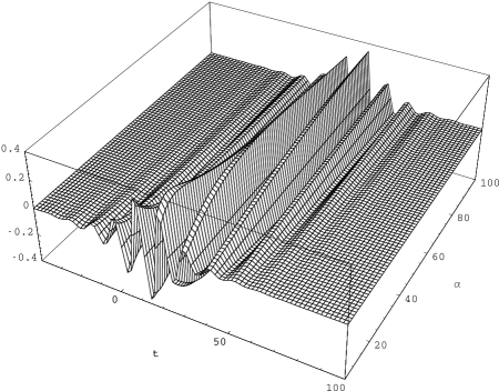
FIG. 1.: $\langle x\rangle$ as a function of time and the parameter $\alpha$, $5\leq\alpha\leq 100$, which controls the initial condition. The moment of SS moves towards the future (past) as $|\alpha|$ grows (decreases). For $|\alpha|=\infty$ ($\alpha=0$) SS is shifted to $+(-)\infty$ (no scattering).

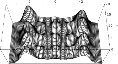
FIG. 2.: The Harzian. Probability density in position space as a function of time for $k=2.5$, $\alpha=5$, $0<t<20$. The asymmetry of the probability density is responsible for the oscillation of $\langle x\rangle$ seen at Fig. 1.

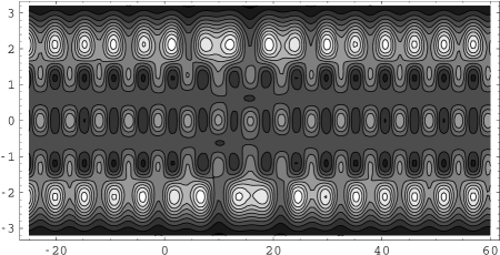
FIG. 3.: Contour plot of the Harzian from Fig. 2 for $-25<t<60$. The continuous transition between the two asymptotic states (with symmetric probability distributions) is clearly visible.

REFERENCES

• [1] F. Cooper, A. Khare, and U. Sukhatme, Phys. Rep. 251, 267 (1995), and references therein.
• [2] V. B. Matveev, M. A. Salle, Darboux Transfomations and Solitons (Springer, Berlin, 1991).
• [3] S. B. Leble and N. V. Ustinov, in Nonlinear Theory and its Applications (NOLTA ’93), p. 547 (Hawaii, 1993); A. A. Zaitsev and S. B. Leble, Rep. Math. Phys. 39, 177 (1997); S. B. Leble, Computers Math. Applic. 35, 73 (1998).
• [4] N. V. Ustinov, J. Math. Phys. 39, 976 (1998).
• [5] S. B. Leble and M. Czachor, Phys. Rev. E 58, 7091 (1998).
• [6] M. Kuna, M. Czachor, and S. B. Leble, Phys. Lett. A 255, 42 (1999).
• [7] M. Czachor, M. Kuna, S. B. Leble, and J. Naudts, in New Insights in Quantum Mechanics, H.-D. Doebner et al. eds. (World Scientific, Singapore, 1999); quant-ph/9904110.
• [8] S. P. Novikov, S. V. Manakov, L. P. Pitaevski, and V. E. Zakharov, Theory of Solitons, the Inverse Scattering Method (Consultants Bureau, New York, 1984).
• [9] M. Czachor and J. Naudts, Phys. Rev. E 59, 2497R (1999).
• [10] S. L. McCall and E. L. Hahn, Phys. Rev. Lett. 18, 908 (1967).
• [11] A. Rahman and J. H. Eberly, Phys. Rev. A 58, R805 (1998).
• [12] The mountain range shape from Fig. 2 sugested an association with the Harz Mountains, where Arnold Sommerfeld Institute is located and this work was done.
• [13] L. J. Mason and N. M. J. Woodhouse, Integrability, Self-Duality, and Twistor Theory (Oxford, 1996).
Refer to caption