Magnetic trapping of neutral particles: Classical and Quantum-mechanical study of a Ioffe-Pritchard type trap.

Abstract

Recently, we developed a method for calculating the lifetime of a particle inside a magnetic trap with respect to spin flips, as a first step in our efforts to understand the quantum-mechanics of magnetic traps. The 1D toy model that was used in this study was physically unrealistic because the magnetic field was not curl-free. Here, we study, both classically and quantum-mechanically, the problem of a neutral particle with spin $S$, mass $m$ and magnetic moment $\mu$, moving in 3D in an inhomogeneous magnetic field corresponding to traps of the Ioffe-Pritchard, ‘clover-leaf’ and ‘baseball’ type. Defining by $\omega_{p}$, $\omega_{z}$ and $\omega_{r}$ the precessional, the axial and the lateral vibrational frequencies, respectively, of the particle in the adiabatic potential $V_{eff}=\mu\left|\mathbf{B}\right|$, we find classically the region in the $\left(\omega_{r}/\omega_{p}\right)$-$\left(\omega_{z}/\omega_{p}\right)$ plane where the particle is trapped.

Quantum-mechanically, we study the problem of a spin-one particle in the same field. Treating $\omega_{r}/\omega_{p}$ and $\omega_{z}/\omega_{p}$ as small parameters for the perturbation from the adiabatic Hamiltonian, we derive a closed-form expression for the transition rate $1/T_{esc}$ of the particle from its trapped ground-state. In the extreme cases the expression for $1/T_{esc}$ reduces to

$$\dfrac{1}{T_{esc}}\simeq\left\{\begin{array}[c]{c}4\pi\omega_{r}\exp\left[-\dfrac{2\omega_{p}}{\omega_{r}}\right]\text{; for }\omega_{p}\gg\omega_{r}\gg\omega_{z}\\ 8\sqrt{2\pi}\sqrt{\omega_{p}\omega_{i}}\exp\left[-\dfrac{2\omega_{p}}{\omega_{i}}\right]\text{ ; for }\omega_{p}\gg\omega_{r}=\omega_{z}\equiv\omega_{i}\\ \sqrt{\dfrac{\pi}{2}}\omega_{r}\left(\dfrac{\omega_{z}}{\omega_{p}}\right)^{3/2}\exp\left[-\dfrac{2\omega_{p}}{\omega_{z}}\right]\text{; for }\omega_{p}\gg\omega_{z}\gg\omega_{r}\end{array}\right..$$

1 Introduction.

1.1 Magnetic traps for neutral particles.

Recently there has been rapid progress in techniques for trapping samples of neutral atoms at elevated densities and extremely low temperatures. The development of magnetic and optical traps for atoms has proceeded in parallel in recent years, in order to attain higher densities and lower temperatures [1, 2, 3, 4, 5]. We should note here that traps for neutral particles have been around much longer than their realizations for neutral atoms might suggest, and the seminal papers for neutral particles trapping as applied to neutrons and plasmas date from the sixties and seventies. Many of these papers are referenced by the authors of Refs.[1, 2, 3]. In this paper we concentrate on the study of magnetic traps. Such traps exploit the interaction of the magnetic moment of the atom with the inhomogeneous magnetic field to provide spatial confinement.

Microscopic particles are not the only candidates for magnetic traps. In fact, a vivid demonstration of trapping large scale objects is the hovering magnetic top [6, 7, 8, 9]. This ingenious magnetic device, which hovers in mid-air for about 2 minutes, has been studied in the past few years by several authors [10, 11, 12, 13, 14, 15].

1.2 Qualitative description.

The physical mechanism underlying the operation of magnetic traps is the adiabatic principle. The common way to describe their operation is in terms of classical mechanics: As the particle is released into the trap, its magnetic moment points antiparallel to the direction of the magnetic field. Inside the trap, the particle experiences translation oscillations with vibrational frequencies $\omega_{vib}$ which are small compared to its precession frequency $\omega_{prec}$. Under this condition the spin of the particle may be considered as experiencing a slowly rotating magnetic field. Thus, the spin precesses around the local direction of the magnetic field $\mathbf{B}$ (adiabatic approximation) and, on the average, its magnetic moment $\mathbf{\mu}$ points antiparallel to the local magnetic field lines. Hence, the magnetic energy, which is normally given by $-\mathbf{\mu}\cdot\mathbf{B}$, is now given (for small precession angle) by $\mu\left|\mathbf{B}\right|$. Thus, the overall effective potential seen by the particle is

$$V_{eff}\simeq\mu\left|\mathbf{B}\right|.$$ (1)

In the adiabatic approximation, the spin degree of freedom is rigidly coupled to the translational degrees of freedom, and is already incorporated in Eq.(1) such that the particle may be considered as having only translational degrees of freedom. When the strength of the magnetic field possesses a minimum, the effective potential becomes attractive near that minimum, and the whole apparatus acts as a trap.

As mentioned above, the adiabatic approximation holds whenever $\omega_{prec}\gg\omega_{vib}$. As $\omega_{prec}$ is inversely proportional to the spin, this inequality can be satisfied provided that the spin of the particle is sufficiently small. If, on the other hand, the spin of the particle is too large, it cannot respond fast enough to the changes of the direction of the magnetic field. In this limit $\omega_{prec}\ll\omega_{vib}$, the spin has to be considered as fixed in space and, according to Earnshaw’s theorem [16], becomes unstable against translations. Note also that $\omega_{prec}$ is proportional to the field $\left|\mathbf{B}\right|$. To prevent $\omega_{prec}$ of becoming too small, resulting in spin-flips (Majorana transitions), most magnetostatic traps include a bias field, so that the effective potential $V_{eff}$ possesses a nonvanishing minimum.

1.3 The purpose and structure of this paper.

The discussion of magnetic traps in the literature is, almost entirely, done in terms of classical mechanics. In microscopic systems, however, quantum effects become important, giving rise to a finite lifetime of the particle within the trap. This requires a quantum-mechanical treatment [17]. An even more interesting issue is the understanding of how the classical and the quantum descriptions of a given system are related. It is important to note here that there are two mechanisms by which the particle can escape from the trap: The first one is the usual tunneling of the particle from the trap, without a change of its spin state, to regions where the magnetic field decreases to zero. The time scale for this process can be evaluated by standard methods. The second way the particle can escape from the trap is by flipping its spin state (Majorana transitions). This process, which is different from the first one because there is no potential barrier, is the subject of this paper.

As a first step in our efforts to understand the quantum-mechanics of magnetic traps, we recently developed a method for calculating the lifetime of a particle inside a magnetic trap with respect to such a spin flip process [18]. The toy model that was used in this study consisted of a particle with spin, having only a single translational degree of freedom, in the presence of a 1D inhomogeneous magnetic field. We found that the trapped state of the particle decays with a lifetime given by $\sim 1/\left(\sqrt{K}\omega_{vib}\right)\exp\left(2/K\right)$ where $K=\omega_{vib}/\omega_{prec}$, and where the result is valid for $K\ll 1$. Though the field that was used in this model did trap the particle, it was not realistic in the sense that it was not curl-free. Our next step was to study the case of a particle with spin, having two translational degree of freedom, in the presence of a physically more realistic trapping field that, in contradistinction to the toy model, is curl-free  [19]. This model is reminiscent of a Ioffe-Pritchard trap [20, 2, 21], but without the axial translational degree of freedom. Here we found that the lifetime is given by $\sim 1/\omega_{vib}\exp\left(2/K\right)$ which is similar to the result found in the 1D case. In the present paper we describe an analysis of a Ioffe-Pritchard type trap which includes the axial translational degree of freedom. We neglect the effect of interactions between the particles in the trap, and we analyze the dynamics of a single particle inside the trap. Unlike in our previous papers, where we studied the case of a spin $1/2$ particle, we treat here the case of a spin $1$ particle, both as an example to show the validity of our approach for higher spins, and also because it is more relevant in view of the recent development in Bose-Einstein condensation experiments.

The structure of this paper is as follows: In Sec.(2) we start by defining the system we study, together with useful parameters that will be used throughout this paper. Next, we carry out a classical analysis of the problem in Sec.(3). Here, we find two stationary solutions for the particle inside the trap. One of them corresponds to a state whose spin is parallel to the direction of the magnetic field whereas the other one corresponds to a state whose spin is antiparallel to that direction. When considering the dynamical stability of these solutions, we find that only the antiparallel stationary solution is stable, as expected from the discussion in Sec.(1.2) above. In Sec.(4) we reconsider the problem from a quantum-mechanical point of view for a spin-one particle. Here, we find states that refer to antiparallel ($M=-1$, where $M$ is the magnetic quantum number) and orthogonal ($M=0$) orientations of the spin, the first of these being bounded while the second one is unbounded. We argue that the third possible situation, in which the spin is parallel ($M=+1$) to the direction of the field, has negligible coupling to the bound state, and therefore can be neglected. We show that the antiparallel and orthogonal states are coupled due to the inhomogeneity of the field, and we calculate the transition rate from the bound state to the unbounded state. Finally, in Sec.(5) we compare the results of the classical analysis with those of the quantum analysis and comment on their implications for practical magnetic traps.

2 Description of the problem.

We consider a particle of mass $m$, magnetic moment $\mu$ and intrinsic spin $S$ (aligned with $\mu$) moving in an inhomogeneous magnetic field $\mathbf{B}$ corresponding to traps of the Ioffe-Pritchard, ‘clover-leaf’ and ‘baseball’ type [2], and given by

$$\mathbf{B} =\left[B_{0}+\dfrac{1}{2}B^{\prime\prime}z^{2}-\dfrac{1}{4}B^{\prime\prime}\left(x^{2}+y^{2}\right)\right]\mathbf{\hat{z}}$$ (2)

$$+\left(B^{\prime}-\dfrac{1}{2}B^{\prime\prime}z\right)x\mathbf{\hat{x}+}\left(-B^{\prime}-\dfrac{1}{2}B^{\prime\prime}z\right)y\mathbf{\hat{y}}\text{.}$$

This field possesses a nonzero minimum of amplitude at the origin, which is the essential part of the trap. The Hamiltonian for this system is

$$H=\dfrac{\mathbf{P}^{2}}{2m}-\mathbf{\mu\cdot B}$$ (3)

where $\mathbf{P}$ is the momentum of the particle.

We define $\omega_{p}$ as the precessional frequency of the particle when it is at the origin $(x=0,y=0,z=0)$. Since at that point the magnetic field is $\mathbf{B=}B_{0}\mathbf{\hat{z}}$ we find that

$$\omega_{p}\equiv\dfrac{\mu B_{0}}{S}\text{.}$$ (4)

Next, we define $\omega_{z}$ and $\omega_{r}$ as the small-amplitude axial and lateral vibrational frequencies of the particle when it is placed with antiparallel spin into the adiabatic potential given by

$$V_{eff}=\mu\left|\mathbf{B}\right|\simeq\mu B_{0}\left(1+\dfrac{B_{0}B^{\prime\prime}}{2B_{0}^{2}}z^{2}+\left(\dfrac{(B^{\prime})^{2}-\frac{1}{2}B_{0}B^{\prime\prime}}{2B_{0}^{2}}\right)r^{2}\right)+\mathcal{O}\left(x^{4},x^{2}y^{2},y^{4}\right),$$

from which we get

$$\omega_{z} \equiv\sqrt{\dfrac{\mu B^{\prime\prime}}{m}}$$ (5)

$$\omega_{r} \equiv\sqrt{\dfrac{\mu\left[(B^{\prime})^{2}-\frac{1}{2}B_{0}B^{\prime\prime}\right]}{mB_{0}}}\text{.}$$

In what follows we assume that $(B^{\prime})^{2}-\frac{1}{2}B_{0}B^{\prime\prime}>0$ such that $\omega_{r}$ is real. We also define the ratios,

$$K_{z} \equiv\dfrac{\omega_{z}}{\omega_{p}}=\sqrt{\dfrac{B^{\prime\prime}S^{2}}{\mu mB_{0}^{2}}}$$ (6)

$$K_{r} \equiv\dfrac{\omega_{r}}{\omega_{p}}=\sqrt{\dfrac{\left[(B^{\prime})^{2}-\frac{1}{2}B_{0}B^{\prime\prime}\right]S^{2}}{\mu mB_{0}^{3}}}$$

These parameters will be our ‘measure of adiabaticity’. It is clear that as $K_{z}$ and $K_{r}$ become smaller and smaller, the adiabatic approximation becomes more and more accurate. Note that when the bias field $B_{0}$ vanishes, both $K_{z}$ and $K_{r}$ become infinite, and the adiabatic approximation fails. We will show below that, under this condition, the system becomes unstable against spin flips, which is in agreement with our discussion at the beginning. This shows that the introduction of the bias field $B_{0}$, is essential to the operation of the trap with regard to spin-flips.

3 Classical analysis.

3.1 The stationary solutions.

We denote by $\mathbf{\hat{n}}$ a unit vector in the direction of the spin (and the magnetic moment). Thus, the equations of motion for the center of mass of the particle are

$$m\dfrac{d^{2}x}{dt^{2}} =\mu\dfrac{\partial}{\partial x}\left(\mathbf{\hat{n}\cdot B}\right)$$ (7)

$$m\dfrac{d^{2}y}{dt^{2}} =\mu\dfrac{\partial}{\partial y}\left(\mathbf{\hat{n}\cdot B}\right)$$

$$m\dfrac{d^{2}z}{dt^{2}} =\mu\dfrac{\partial}{\partial z}\left(\mathbf{\hat{n}\cdot B}\right)$$

and the evolution of its spin is determined by

$$S\dfrac{d\mathbf{\hat{n}}}{dt}=\mu\mathbf{\hat{n}\times B}\text{.}$$ (8)

The two equilibrium solutions to Eqs.(7) and (8) are

$$\mathbf{\hat{n}}(t)=\mp\mathbf{\hat{z}}$$ (9)

with

$$x(t) =0$$

$$y(t) =0$$

$$z\left(t\right) =0$$

representing a motionless particle at the origin with its magnetic moment (and spin) pointing antiparallel ($\mathbf{\hat{n}}(t)=-\mathbf{\hat{z}}$) to the direction of the field at that point and a similar solution but with the magnetic moment pointing parallel to the direction of the field ($\mathbf{\hat{n}}(t)=+\mathbf{\hat{z}}$).

3.2 Stability of the solutions.

To check the stability of these solutions we now add first-order perturbations. We set

$$\mathbf{\hat{n}(}t\mathbf{)} =\mathbf{\mp\hat{z}+}\epsilon_{x}(t)\mathbf{\hat{x}+}\epsilon_{y}(t)\mathbf{\hat{y}}$$ (10)

$$x(t) =0+\delta x(t)$$

$$y(t) =0+\delta y(t)$$

$$z(t) =0+\delta z(t)$$

(note that, to first order, the perturbation $\delta\mathbf{\hat{n}}=\epsilon_{x}(t)\mathbf{\hat{x}+}\epsilon_{y}(t)\mathbf{\hat{y}}$ is orthogonal to the vector $\mathbf{\hat{n}}$ for the stationary solution $\mathbf{\hat{n}}_{0}=\mathbf{\mp\hat{z}}$, since $\mathbf{\hat{n}}$ is a unit vector), substitute these into Eqs.(7) and (8), and retain only first-order terms. We find that the resulting equations for $\delta x(t)$, $\delta y(t)$, $\delta z\left(t\right)$, $\epsilon_{x}(t)$ and $\epsilon_{y}(t)$ are

$$m\dfrac{d^{2}\delta x}{dt^{2}} =\pm\dfrac{1}{2}\mu B^{\prime\prime}\delta x+\mu B^{\prime}\epsilon_{x}$$ (11)

$$m\dfrac{d^{2}\delta y}{dt^{2}} =\pm\dfrac{1}{2}\mu B^{\prime\prime}\delta y-\mu B^{\prime}\epsilon_{y}$$

$$m\dfrac{d^{2}\delta z}{dt^{2}} =\mp\mu B^{\prime\prime}\delta z$$

$$S\dfrac{d\epsilon_{x}}{dt} =\mu B_{0}\epsilon_{y}\mp\mu B^{\prime}\delta y$$

$$S\dfrac{d\epsilon_{y}}{dt} =-\mu B_{0}\epsilon_{x}\mp\mu B^{\prime}\delta x.$$

The motion of the $z$-coordinate is decoupled from the others. If $B^{\prime\prime}>0$, it is stable only when the upper sign is taken, corresponding to a spin antiparallel to the direction of the field. It can be shown that when $B^{\prime\prime}<0$ then, even if the system is stable under axial vibrations (by choosing the lower sign), it cannot be stable as a whole. We therefore disregard the lower sign, and the equation for the $z$-coordinate for the rest of the derivation.

The normal modes of the reduced system transform as the irreducible representations of the symmetry group. The 4-dimensional linear space spanned by the deviations $(\delta x,\delta y,\epsilon_{x},\epsilon_{y})$ from the stationary state carries the irreducible representations $\Gamma_{+}$ with characters $e^{-i\gamma}$ and $\Gamma_{-}$ with characters $e^{+i\gamma}$, and may thus be decomposed into the two 2-dimensional invariant subspaces transforming as $\Gamma_{+}$ and $\Gamma_{-}$, respectively. These subspaces are spanned by the circular position coordinates and precessional spin coordinates

$$\Gamma_{+}:\; (\rho_{+}=\delta x+i\delta y,\epsilon_{-}=\epsilon_{x}-i\epsilon_{y});$$ (12)

$$\Gamma_{-}:\; (\rho_{-}=\delta x-i\delta y,\epsilon_{+}=\epsilon_{x}+i\epsilon_{y}).$$ (13)

Thus, the normal modes consist of a circular motion in the $(x,y)$-plane coupled to a precession of the spin vector in the opposite sense.

Indeed, after introducing the $(\rho_{\pm},\epsilon_{\mp})$-coordinates into Eqs.(11), this set of four equations decomposes into one pair of equations for $(\rho_{+},\epsilon_{-})$ and another pair for $(\rho_{-},\epsilon_{+})$. We now look for oscillatory (stable) solutions of these equations and set

$$\rho_{\pm}=\rho_{\pm,0}e^{-i\omega t},\quad\epsilon_{\pm}=\epsilon_{\pm,0}e^{-i\omega t}.$$ (14)

This yields the algebraic equations

$$\Gamma_{+}:\;\left(\begin{array}[c]{cc}\dfrac{1}{2}\mu B^{\prime\prime}+m\omega^{2}&\mu B^{\prime}\\ i\mu B^{\prime}&i\left(\omega S+\mu B_{0}\right)\end{array}\right)\cdot\left(\begin{array}[c]{l}\rho_{+,0}\\ \epsilon_{-,0}\end{array}\right)=\left(\begin{array}[c]{l}0\\ 0\end{array}\right),$$ (15)

$$\Gamma_{-}:\;\left(\begin{array}[c]{cc}\dfrac{1}{2}\mu B^{\prime\prime}+m\omega^{2}&\mu B^{\prime}\\ -i\mu B^{\prime}&i\left(\omega S-\mu B_{0}\right)\end{array}\right)\cdot\left(\begin{array}[c]{l}\rho_{-,0}\\ \epsilon_{+,0}\end{array}\right)=\left(\begin{array}[c]{l}0\\ 0\end{array}\right).$$ (16)

These equations have non-trivial solutions whenever the determinant of either of the two matrices vanishes. This yields the secular equations

$$\Gamma_{+} :\left(\frac{\omega}{\omega_{p}}\right)^{3}+\left(\frac{\omega}{\omega_{p}}\right)^{2}+\dfrac{1}{2}K_{z}^{2}\left(\frac{\omega}{\omega_{p}}\right)-K_{r}^{2}=0,$$ (17)

$$\Gamma_{-} :\;\left(\frac{\omega}{\omega_{p}}\right)^{3}-\left(\frac{\omega}{\omega_{p}}\right)^{2}+\dfrac{1}{2}K_{z}^{2}\left(\frac{\omega}{\omega_{p}}\right)+K_{r}^{2}=0,$$ (18)

which determine the eigenfrequencies $\omega$ of the various modes. Since the reduced system has three degrees of freedom, we expect to have three normal modes. Indeed, when $\omega$ is a solution of the first equation, then $-\omega$ is a solution of the second equation. We define the mode frequencies in Eq.(17) to be positive (or, in the case of complex $\omega$, to have positive real part); the negative $\omega$-values are needed to construct real solutions. Then, the $\Gamma_{+}$-modes describe vibrational motions turning counter-clockwise coupled to spin precessions turning clockwise, i.e., opposite to the natural spin precession, and the $\Gamma_{-}$-modes describe vibrational motions turning clockwise coupled to spin precessions turning counter-clockwise, i.e., in the same sense as the natural spin precession.

Stability requires that all three solutions of, say, Eq.(18) be real. We note that at the edge of the stability region (and when $K_{r}\neq 0$), two out of the three roots of Eq.(18) for $\omega$ become identical. In this case, the third order polynomial Eq.(18) takes the form $P\left(\omega\right)=\left(\omega-\omega_{1}\right)^{2}$ $\left(\omega-\omega_{2}\right)$, which satisfy $\left.dP/d\omega\right|_{\omega=\omega_{1}}=0$. The edge of the stability region is then found by simultaneously solving the equations $P\left(\omega\right)=0$ and $dP/d\omega=0$. The result is given in the form of the parametric curve in the $(K_{r}^{2},K_{z}^{2})$-plane

$$\left\{\begin{array}[c]{c}K_{r}^{2}\left(t\right)=2t^{3}-t^{2}\\ K_{z}^{2}\left(t\right)=4t-6t^{2}\end{array}\right\}\text{ ; with }\dfrac{1}{2}<t<\dfrac{2}{3}$$

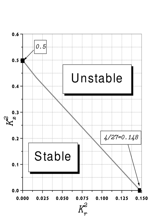
Figure 1: Stable region in the $(K_{r}^{2},K_{z}^{2})$-plane, as predicted by the classical analysis.

which is shown in Fig.(1). Note that by eliminating $t$ from the second equation and substituting it in the first gives $K_{r}^{2}$ explicitly in terms of $K_{z}^{2}$.

4 Quantum-mechanical analysis.

4.1 The Hamiltonian and its diagonalized form.

In this section we consider the problem of a neutral particle with spin one ($S=\hbar$) in a 3D inhomogeneous magnetic field from a quantum-mechanical point of view. Unlike the classical analysis, in which the derivation was valid for any value of the adiabaticity parameters $K_{r}$ and $K_{z}$, we concentrate here on the behavior of the system when $K_{r}$ and $K_{z}$ are small. Note also that, quantum-mechanically, the magnetic moment $\mu$ and the spin $S$ of a particle are related by

$$\mu=\gamma S,$$

where $\gamma$ is the gyromagnetic ratio of the particle. Setting $\mu=\gamma S$ and $S=\hbar$ in Eqs.(6) gives

$$K_{z} =\dfrac{\omega_{p}}{\omega_{z}}=\sqrt{\dfrac{B^{\prime\prime}\hbar}{\gamma mB_{0}^{2}}}$$

$$K_{r} =\dfrac{\omega_{p}}{\omega_{r}}=\sqrt{\dfrac{\left[(B^{\prime})^{2}-\frac{1}{2}B_{0}B^{\prime\prime}\right]\hbar}{\gamma mB_{0}^{3}}}.$$

Now, it is convenient to transform to cylindrical coordinates $(r,\phi,z)$ by setting $x=r\cos\phi$, $y=r\sin\phi$. We denote by $B$ the amplitude of $\mathbf{B}$, by $\theta$ its direction with respect to the $z$-axis and by $\varphi$ the angle between the projection of $\mathbf{B}$ onto the $\left(x,y\right)$-plane and the $x$-axis. Thus, Eq.(2) is rewritten as

$$\mathbf{B}=B\left[\sin\theta\cos\varphi\mathbf{\hat{x}+}\sin\theta\sin\varphi\mathbf{\hat{y}}+\cos\theta\mathbf{\hat{z}}\right].$$ (19)

The approximate expressions for $B$, $\theta$ and $\varphi$ near the origin are given by

$$B\left(r,\phi,z\right) \simeq B_{0}\left(1+\dfrac{B_{0}B^{\prime\prime}}{2B_{0}^{2}}z^{2}+\left(\dfrac{(B^{\prime})^{2}-\frac{1}{2}B_{0}B^{\prime\prime}}{2B_{0}^{2}}\right)r^{2}\right)\text{ }+\mathcal{O}\left(r^{4},z^{2}r^{2},z^{4}\right)\text{,}$$ (20)

$$\theta\left(r,\phi,z\right) =\arctan\left(\dfrac{\sqrt{B_{x}^{2}+B_{y}^{2}}}{B_{z}}\right)\simeq\dfrac{B^{\prime}r}{B_{0}}+\mathcal{O}\left(r^{2},rz,z^{2}\right)\text{,}$$

$$\varphi\left(r,\phi,z\right) =\arctan\left(\dfrac{B_{y}}{B_{x}}\right)\simeq\arctan\left(-\dfrac{y}{x}\left[1+\left(\frac{B^{\prime\prime}}{B^{\prime}}\right)z\right]\right)\simeq-\phi+\mathcal{O}\left(z\sin\left(2\phi\right)\right).$$

Thus approximately, $B$ and $\theta$ depend only on $r$, whereas $\varphi$ depends only linearly on $\phi$.

The time-independent Schrödinger equation for this system is

$$\left[-\frac{\hbar^{2}}{2m}\nabla^{2}-\mu B\left(\sin\theta\cos\varphi\hat{s}_{x}\mathbf{+}\sin\theta\sin\varphi\hat{s}_{y}+\cos\theta\hat{s}_{z}\right)\right]\Phi(r,\phi,z)=E\Phi(r,\phi,z)$$ (21)

where $\hat{s}_{x}$, $\hat{s}_{y}$ and $\hat{s}_{z}$ are the spin one matrices, given by

$$\begin{array}[c]{ccc}\hat{s}_{x}=\dfrac{1}{\sqrt{2}}\left(\begin{array}[c]{lll}0&1&0\\ 1&0&1\\ 0&1&0\end{array}\right)&\hat{s}_{y}=\dfrac{1}{\sqrt{2}}\left(\begin{array}[c]{lll}0&-i&0\\ i&0&-i\\ 0&i&0\end{array}\right)&\hat{s}_{z}=\left(\begin{array}[c]{lll}1&0&0\\ 0&0&0\\ 0&0&-1\end{array}\right),\end{array}$$

$E$ is the eigenenergy, and $\Phi$ is the three-components spinor

$$\Phi=\left(\begin{array}[c]{c}\Phi_{+}(r,\phi,z)\\ \Phi_{0}(r,\phi,z)\\ \Phi_{-}(r,\phi,z)\end{array}\right).$$ (22)

In matrix form Eq.(21) becomes

$$\left(H_{K}+H_{M}\right)\left(\begin{array}[c]{c}\Phi_{+}(r,\phi,z)\\ \Phi_{0}(r,\phi,z)\\ \Phi_{-}(r,\phi,z)\end{array}\right)=E\left(\begin{array}[c]{c}\Phi_{+}(r,\phi,z)\\ \Phi_{0}(r,\phi,z)\\ \Phi_{-}(r,\phi,z)\end{array}\right),$$ (23)

where $H_{K}$ and $H_{M}$, given by

$$H_{K} \equiv-\dfrac{\hbar^{2}}{2m}\nabla^{2}$$ (24)

$$H_{M} \equiv-\mu B\left(\begin{array}[c]{lll}\cos\theta&\dfrac{1}{\sqrt{2}}\sin\theta e^{-i\varphi}&0\\ \dfrac{1}{\sqrt{2}}\sin\theta e^{i\varphi}&0&\dfrac{1}{\sqrt{2}}\sin\theta e^{-i\varphi}\\ 0&\dfrac{1}{\sqrt{2}}\sin\theta e^{i\varphi}&-\cos\theta\end{array}\right),$$ (28)

are the kinetic part and the magnetic part of the Hamiltonian $H$, respectively.

In order to diagonalize the magnetic part of the Hamiltonian, we make a local passive transformation of coordinates on the wavefunction such that the spinor is expressed in a new coordinate system whose $\mathbf{\hat{z}}$ axis coincides with the direction of the magnetic field at the point $\left(r,\phi,z\right)$. We denote by $R\left(r,\phi,z\right)$ the required transformation and set $\Psi=R\Phi$. Thus, $\Psi$ represent the same direction of the spin as before the transformation but using the new coordinate system. The Hamiltonian in this newly defined system is given by $RHR^{-1}$. We represent the rotation matrix $R$ in terms of the three Euler angles: First, we perform a rotation through an angle $\varphi$ around the $\hat{z}$ axis. Second, we make a rotation through an angle $\theta$ around the new position of the $\hat{y}$ axis. At the end of this process the new $\hat{z}$ axis coincide with the direction of the magnetic field. Now the value of the last Euler angle, which is a rotation around the new $\hat{z}$ axis, has no effect on this axis. For simplicity we choose this angle to be $0$. Thus, the representation of the complete transformation for spin-one particle is given by [22]

$$R=\exp\left[i\theta\hat{s}_{y}\right]\exp\left[i\varphi\hat{s}_{z}\right],$$

while its inverse is given by

$$R^{-1}=\exp\left[-i\varphi\hat{s}_{z}\right]\exp\left[-i\theta\hat{s}_{y}\right].$$

It is easily verified that the transformation indeed diagonalizes the magnetic part of the Hamiltonian as

$$RH_{M}R^{-1}=-\mu B\hat{s}_{z}.$$

As for the kinetic part we show at the Appendix that

$$RH_{K}R^{-1}=-\dfrac{\hbar^{2}}{2m}\left[\begin{array}[c]{c}-i\nabla^{2}\varphi\left(\cos\theta\hat{s}_{z}-\sin\theta\hat{s}_{x}\right)-\left|\nabla\varphi\right|^{2}\left(\cos\theta\hat{s}_{z}-\sin\theta\hat{s}_{x}\right)^{2}\\ -2i\left(\cos\theta\hat{s}_{z}-\sin\theta\hat{s}_{x}\right)\nabla\varphi\cdot\left(-i\mathbf{\nabla}\theta\hat{s}_{y}+\mathbf{\nabla}\right)\\ -i\nabla^{2}\theta\hat{s}_{y}-\left|\mathbf{\nabla}\theta\right|^{2}\hat{s}_{y}^{2}-2i\hat{s}_{y}\mathbf{\nabla}\theta\cdot\nabla+\nabla^{2}\end{array}\right].$$ (29)

Since we are interested in the behavior near the origin, we substitute the approximate expressions Eqs.(20) into Eq.(29), replace $\cos\theta$ by $1$ and $\sin\theta$ by $0$ (since $\theta$ changes very slowly as compared to the extent over which $\mu B$ changes significantly), and neglect the terms that are proportional to $\nabla^{2}\theta$ and $\left|\mathbf{\nabla}\theta\right|^{2}$ (being of higher order with respect to $\mathbf{\nabla}\theta\cdot\nabla$ ). This gives

$$RH_{K}R^{-1}\simeq-\dfrac{\hbar^{2}}{2m}\left[\nabla^{2}-2i\hat{s}_{y}\dfrac{B^{\prime}}{B_{0}}\dfrac{\partial}{\partial r}+2i\dfrac{1}{r^{2}}\hat{s}_{z}\dfrac{\partial}{\partial\phi}-\dfrac{1}{r^{2}}\hat{s}_{z}^{2}\right]\text{.}$$

Thus, the Hamiltonian of the system in the rotated frame may be written approximately as

$$H\simeq H_{diag}+H_{int}\text{,}$$ (30)

where

$$H_{diag} =-\dfrac{\hbar^{2}}{2m}\left[\mathbf{\nabla}^{2}+\dfrac{2i}{r^{2}}\hat{s}_{z}\dfrac{\partial}{\partial\phi}-\dfrac{1}{r^{2}}\hat{s}_{z}^{2}\right]-\mu B\hat{s}_{z}$$ (31)

$$H_{int} =i\dfrac{\hbar^{2}B^{\prime}}{mB_{0}}\hat{s}_{y}\dfrac{\partial}{\partial r}.$$

The first part of the Hamiltonian $H_{diag}$ is diagonal with respect to the spin degrees of freedom. It contains the kinetic part $\sim\mathbf{\nabla}^{2}$, a term whose form is $-\mu B\hat{s}_{z}$ which is identified as the adiabatic effective potential, and the terms $\sim 1/r^{2},ir^{-2}\hat{s}_{z}\partial/\partial\phi$ which appear due to the rotation. The second part of the Hamiltonian $H_{int}$ contains only non-diagonal components. Generally, $H_{int}$ should contain terms which couple a spin state $M$ to the two nearest spin states $M\pm 1$ and to the two next-to-nearest spin states $M\pm 2$ (see the Appendix). In the limit where $K_{z}$ and $K_{r}$ are small, we see that the coupling of the state with spin projection value $M$ to the states $M\pm 2$ is negligible compared to its coupling to the $M\pm 1$ states. We proceed to find the eigenstates of $H_{diag}$.

4.2 Stationary states of $H_{diag}$.

Since $H_{diag}$ is diagonal, the three spin states of the wavefunction are decoupled. We seek a solution for the spin-down ($M=-1$) state

$$\Psi_{-}=\left(\begin{array}[c]{c}0\\ 0\\ \psi_{-}(r,\phi,z)\end{array}\right)\text{ ; }E=E_{-},$$ (32)

and for the $M=0$ state

$$\Psi_{0}=\left(\begin{array}[c]{c}0\\ \psi_{0}(r,\phi,z)\\ 0\end{array}\right)\text{ ; }E=E_{0}.$$ (33)

We do not consider the spin-up ($M=+1$) state, since its coupling to the trapped spin-down state is negligible, as explained above.

The equation for the non-vanishing component of the spin-down state reads

$$\left\{-\dfrac{\hbar^{2}}{2m}\left[\mathbf{\nabla}^{2}-\dfrac{2i}{r^{2}}\dfrac{\partial}{\partial\phi}-\dfrac{1}{r^{2}}\right]+\mu B\right\}\psi_{-}=E_{-}\psi_{-},$$ (34)

whereas the equation for the non-vanishing component of the spin-zero state is

$$-\dfrac{\hbar^{2}}{2m}\mathbf{\nabla}^{2}\psi_{0}=E_{0}\psi_{0}.$$ (35)

The solutions of these equations is outlined in the next two subsections.

4.2.1 Stationary spin-down ($M=-1$) states.

Eq.(34) represents a particle in a cylindrically symmetric attractive 3D potential. If the extent of the wave function is small enough we can expand $B$ in Eq.(20) to second order in $r$ and $z$ as given by Eq.(20), and apply the well-known solution of the harmonic oscillator [23] in 3D. Under this approximation, Eq.(34) becomes

$$\left\{\begin{array}[c]{c}-\dfrac{\hbar^{2}}{2m}\left(\dfrac{\partial^{2}}{\partial z^{2}}+\dfrac{\partial^{2}}{\partial r^{2}}+\dfrac{1}{r}\dfrac{\partial}{\partial r}-\dfrac{1}{r^{2}}\left(i\dfrac{\partial}{\partial\phi}+1\right)^{2}\right)\\ +\left[\dfrac{m\omega_{z}^{2}}{2}z^{2}+\dfrac{m\omega_{r}^{2}}{2}r^{2}\right]\end{array}\right\}\psi_{-}=\left(E_{-}-\mu B_{0}\right)\psi_{-}.$$ (36)

The $z$-coordinate decouples and we assume that it is in the ground-state. We thus seek a solution whose form is

$$\psi_{-}(r,z,\phi)=f(r)e^{i\nu\phi}\left(\dfrac{m\omega_{z}}{\pi\hbar}\right)^{1/4}\exp\left[-\dfrac{m\omega_{z}z^{2}}{2\hbar}\right],$$ (37)

with $\nu$ an integer. The equation satisfied by $f\left(r\right)$ is then

$$-\dfrac{\hbar^{2}}{2m}\left[\dfrac{d^{2}f}{dr^{2}}+\dfrac{1}{r}\dfrac{df}{dr}-\dfrac{f}{r^{2}}\left(\nu-1\right)^{2}\right]+\dfrac{m\omega_{r}^{2}r^{2}}{2}f=\left(E_{-}-\mu B_{0}-\dfrac{1}{2}\hbar\omega_{z}\right)f.$$ (38)

This is an eigenvalue problem for $f$. The smallest eigenvalue for this equation is obtained by setting

$$\nu=1,$$

for which the eigenfunction $f$ is

$$f\left(r\right)=De^{i\phi}\exp\left[-\dfrac{m\omega_{r}}{2\hbar}r^{2}\right].$$

Thus, under the harmonic-oscillator approximation, the normalized down-part of the spin-down state is given by

$$\psi_{-}=\sqrt{\dfrac{m\omega_{r}}{\pi\hbar}}\text{ }\left(\dfrac{m\omega_{z}}{\pi\hbar}\right)^{1/4}e^{i\phi}\exp\left[-\dfrac{m\omega_{r}}{2\hbar}r^{2}\right]\exp\left[-\dfrac{m\omega_{z}}{2\hbar}z^{2}\right].$$ (39)

Note that the extent of this wave function over which it changes appreciably is given by

$$\Delta z\sim\sqrt{K_{z}}\sqrt{\dfrac{B_{0}}{B^{\prime\prime}}}\text{ ; }\Delta r\sim\sqrt{K_{r}}\sqrt{\dfrac{B_{0}}{B^{\prime\prime}}}$$ (40)

whereas the extent over which $\mu B$ changes significantly (see Eq.(20)) is

$$\Delta r_{\mu B}\sim\sqrt{\dfrac{B_{0}}{B^{\prime\prime}}}.$$ (41)

Thus, the ratio between these two length scales is

$$\dfrac{\Delta z}{\Delta r_{\mu B}}\sim\sqrt{K_{z}}\text{ ; }\dfrac{\Delta r}{\Delta r_{\mu B}}\sim\sqrt{K_{r}}.$$ (42)

We therefore conclude that when $K_{z}$ and $K_{r}$ are small enough, the harmonic approximation is justified.

The wave function $\psi_{-}$, given by Eq.(39), then represents the lowest possible bound state for this system. This state corresponds to a trapped particle. The energy of this state is

$$E_{-}=\mu B_{0}+\dfrac{1}{2}\hbar\omega_{z}+\hbar\omega_{r}=\mu B_{0}\left(1+K_{z}+2K_{r}\right)\simeq\mu B_{0},$$ (43)

while its full spinor representation is

$$\Psi_{-}=\left(\begin{array}[c]{c}0\\ 0\\ \sqrt{\dfrac{m\omega_{r}}{\pi\hbar}}\text{ }\left(\dfrac{m\omega_{z}}{\pi\hbar}\right)^{1/4}e^{i\phi}\exp\left[-\dfrac{m\omega_{r}}{2\hbar}r^{2}\right]\exp\left[-\dfrac{m\omega_{z}}{2\hbar}z^{2}\right]\end{array}\right).$$ (44)

4.2.2 Stationary ($M=0$) states.

Eq.(35) describes a free particle. It corresponds to an unbounded state representing an untrapped particle. In this case there is a continuum of states, each with its own energy. As we are interested in non-radiative decay, we focus on finding a solution with an energy which is equal to the energy found for the trapped state, that is

$$E_{0}=E_{-}\simeq\mu B_{0}.$$ (45)

We seek a solution in the form

$$\psi_{0}(r,\phi)=g(r)\exp\left[ik_{z}z+i\beta\phi\right],$$

where $\beta$ is an integer. Substituting this, together with Eq.(45) into Eq.(35) gives

$$\left[\dfrac{d^{2}}{dr^{2}}+\dfrac{1}{r}\dfrac{d}{dr}+\left(k_{r}^{2}-\dfrac{\beta^{2}}{r^{2}}\right)\right]g=0,$$

where

$$k_{r}^{2}+k_{z}^{2}=\dfrac{2\mu mB_{0}}{\hbar^{2}}\text{.}$$

The non-singular solution for $g$ is

$$g\left(r\right)=J_{\beta}\left(k_{r}r\right),$$

where $J_{\beta}\left(x\right)$ is the Bessel function of the first kind of order $\beta$. For what follows, it is convenient to introduce an angle $\gamma$ such that

$$k_{r} =k_{0}\sin\gamma$$

$$k_{z} =k_{0}\cos\gamma.$$

$$k_{0} \equiv\sqrt{\dfrac{2\mu mB_{0}}{\hbar^{2}}}$$

with $0<\gamma<\pi$.

We note that $H_{int}$ does not operate on the $\phi$ coordinate. Hence, in order to have a non-vanishing matrix element between the zero-state and the down-state, they must have the same $\phi$-dependence. Thus, $\beta=\nu=1$, and as a result, the state with angle $\gamma$ is given by

$$\psi_{0}^{\gamma}(r,\phi,z)=C_{\gamma}J_{1}\left(k_{0}r\sin\gamma\right)\exp\left[i\left(\phi+k_{0}z\cos\gamma\right)\right]\text{.}$$ (46)

with

$$\Psi_{0}^{\gamma}=\left(\begin{array}[c]{c}0\\ C_{\gamma}J_{1}\left(k_{0}r\sin\gamma\right)\exp\left[i\left(\phi+k_{0}z\cos\gamma\right)\right]\\ 0\end{array}\right),\text{ }$$ (47)

where $C_{\gamma}$ is the normalization constant which is chosen to be real, and depends on $\gamma$. To evaluate $C_{\gamma}$ we temporarily introduce boundary conditions under which the wavefunction $\Psi_{0}^{\gamma}$ vanishes at $r=R$, and satisfies periodic boundary conditions along $z$ with period $Z$. Thus, normalization of $\Psi_{0}^{\gamma}$ gives

$$\int_{-Z/2}^{Z/2}dz\int_{0}^{2\pi}d\phi\int_{0}^{R}rdr\left|\Psi_{0}^{\gamma}\right|^{2}=C_{\gamma}^{2}Z2\pi\frac{1}{2}R^{2}[J_{2}(k_{0}R\sin\gamma)]^{2}=1,$$

such that

$$C_{\gamma}=\dfrac{1}{\sqrt{Z\pi}R\left|J_{2}(k_{0}R\sin\gamma)\right|},$$

where we have used [24]

$$\int_{0}^{R}[J_{1}(kr)]^{2}rdr=\frac{1}{2}R^{2}[J_{2}(kR)]^{2}.$$

In the asymptotic region $kR\gtrsim 1$, the function $J_{2}(kR)$ takes the values $\pm\sqrt{2/(\pi kR)}$ at the zeros of $J_{1}(kR)$. Thus,

$$C_{\gamma}=\dfrac{1}{\sqrt{Z\pi}R\left|J_{2}(k_{0}R\sin\gamma)\right|}\simeq\dfrac{\sqrt{k_{0}\sin\gamma}}{\sqrt{2ZR}}$$

and hence

$$C_{\gamma}^{2}\simeq\dfrac{k_{0}\sin\gamma}{2ZR}.$$ (48)

4.3 The transition rate.

We calculate the transition rate from the bound state given by Eq.(44) to the unbounded state Eq.(47), according to Fermi’s golden rule [25]. Thus, the infinitesimal decay time from the trapped state to the untrapped state defined by $\gamma$ is given by

$$d\left(\dfrac{1}{T_{esc}^{\gamma}}\right)=\dfrac{2\pi}{\hbar}\left|H_{i}^{\gamma}\right|^{2}\rho_{\gamma}(E_{0})d\gamma,$$ (49)

where $\rho_{\gamma}(E)d\gamma$ is the density $dN/dE$ of states $\psi_{0}^{\gamma}$ with an angle between $\gamma$ and $\gamma+d\gamma$ and energy between $E_{0}$ and $E_{0}+dE$, and $H_{i}^{\gamma}$ is the matrix element of $H_{int}$ between the bound state and the unbounded state defined by $\gamma$ and $E_{0}$. To find $\rho_{\gamma}(E_{0})$ we note that the final state is defined by the two quantized $k$-vectors $k_{r}=k_{0}\sin\gamma$ and $k_{z}=k_{0}\cos\gamma$. The possible $k_{z}$ values are equally-spaced with lattice constant $dk_{z}=2\pi/Z$. Since the Bessel function $J_{1}(k_{r}r)$ is very close to its asymptotic behavior at large arguments

$$J_{1}(k_{r}R)\simeq\sqrt{\frac{2}{\pi k_{r}R}}\,\cos\left(k_{r}R-\frac{3\pi}{4}\right),$$

the $k_{r}$ are also very much equally-spaced (even when $k_{r}$ is small, it is still a good approximation) with lattice constant $dk_{r}\simeq\pi/R$. Thus, in the $\left(k_{r},k_{z}\right)$-space, the allowed $k$ vectors form a regular lattice, and the number of states $dN$ in the volume element $k_{0}dk_{0}d\gamma$ is given by

$$dN=\dfrac{k_{0}d\gamma dk_{0}}{\left(\dfrac{\pi}{R}\right)\left(\dfrac{2\pi}{Z}\right)}.$$

With $dE=\hbar^{2}k_{0}dk_{0}/m$, this gives the density of states

$$\rho_{\gamma}(E)d\gamma=\dfrac{dN}{dE}\simeq\dfrac{mZR}{2\pi^{2}\hbar^{2}}d\gamma.$$

This, together with Eq.(48) yields

$$C_{\gamma}^{2}\rho_{\gamma}(E)\simeq\dfrac{mk_{0}\sin\gamma}{4\pi^{2}\hbar^{2}}.$$ (50)

Evaluation of $H_{i}^{\gamma}$ gives

$$H_{i}^{\gamma} =\int_{-\infty}^{\infty}dz{\displaystyle\int\limits_{0}^{\infty}}rdr{\displaystyle\int\limits_{0}^{2\pi}}d\phi\Psi_{0}^{\dagger\gamma}H_{int}\Psi_{-}$$

$$=2\pi\sqrt{\dfrac{m\omega_{r}}{\pi\hbar}}\text{ }\left(\dfrac{m\omega_{z}}{\pi\hbar}\right)^{1/4}\left[i\dfrac{\hbar^{2}B^{\prime}}{mB_{0}}\dfrac{\left(-i\right)}{\sqrt{2}}\right]\left(-\dfrac{m\omega_{r}}{\hbar}\right)C_{\gamma}$$

$$\times {\displaystyle\int\limits_{0}^{\infty}}drr^{2}J_{1}\left(k_{0}r\sin\gamma\right)\exp\left[-\dfrac{m\omega_{r}}{2\hbar}r^{2}\right]\int_{-\infty}^{\infty}dz\exp\left[-\dfrac{m\omega_{z}}{2\hbar}z^{2}-ik_{0}z\cos\gamma\right].$$

and hence

$$\left|H_{i}^{\gamma}\right|^{2} =4\pi^{2}\dfrac{m\omega_{r}}{\pi\hbar}\sqrt{\dfrac{m\omega_{z}}{\pi\hbar}}\left(\dfrac{\hbar^{2}B^{\prime}}{\sqrt{2}mB_{0}}\right)^{2}\left(\dfrac{m\omega_{r}}{\hbar}\right)^{2}C_{\gamma}^{2}\dfrac{2\pi\hbar}{m\omega_{z}}\left(\dfrac{k_{0}\hbar^{2}\sin\gamma}{m^{2}\omega_{r}^{2}}\right)^{2}$$ (51)

$$\times\exp\left[-\frac{\hbar k_{0}^{2}\cos^{2}\gamma}{m\omega_{z}}-\dfrac{k_{0}^{2}\hbar\sin^{2}\gamma}{m\omega_{r}}\right].$$

Substituting Eqs.(51) and (50) into Eq.(49) and integrating over $\gamma$ from $0$ to $\pi$ gives

$$\dfrac{1}{T_{esc}}=2\sqrt{2\pi}\frac{\left(2\omega_{r}^{2}+\omega_{z}^{2}\right)\sqrt{\omega_{p}}}{\omega_{r}\sqrt{\omega_{z}}}I\left(\dfrac{2\omega_{p}}{\omega_{r}},\dfrac{2\omega_{p}}{\omega_{z}}\right)$$ (52)

with

$$I\left(a,b\right)\equiv\int_{0}^{\pi}d\gamma\sin^{3}\gamma\exp\left[-a\sin^{2}\gamma-b\cos^{2}\gamma\right],$$ (53)

where we have substituted our previous definitions for $\omega_{p}$, $\omega_{r}$ and $\omega_{z}$. The integral $I\left(a,b\right)$ may be expressed in terms of the simpler integral

$$I_{0}\left(a,b\right) \equiv\int_{0}^{\pi}d\gamma\sin\gamma\exp\left[-a\sin^{2}\gamma-b\cos^{2}\gamma\right]$$ (54)

$$=2\exp\left(-a\right)\int_{0}^{1}\exp\left[\left(a-b\right)t^{2}\right]dt$$

by

$$I\left(a,b\right)=-\dfrac{\partial I_{0}\left(a,b\right)}{\partial a}.$$ (55)

In the isotropic case where $\omega_{r}=\omega_{z}\equiv\omega_{i}$, the integral in Eq.(52) can be evaluated analytically with the result that

$$\dfrac{1}{T_{esc}}=8\sqrt{2\pi}\sqrt{\omega_{p}\omega_{i}}\exp\left[-\frac{2\omega_{p}}{\omega_{i}}\right].$$

In the extreme cases $\omega_{r}\gg\omega_{z}$ and $\omega_{z}\gg\omega_{r}$ we obtain from the asymptotic behavior of the error function of real and imaginary argument [26]

$$I_{0}\left(a,b\right)\simeq\left\{\begin{array}[c]{cc}\sqrt{\dfrac{\pi}{b}}\exp\left(-a\right)&\text{; }b\gg a\\ \dfrac{1}{a}\exp\left(-b\right)&\text{; }b\ll a\end{array}\right.,$$ (56)

and hence

$$I\left(a,b\right)=-\dfrac{\partial I_{0}\left(a,b\right)}{\partial a}\simeq\left\{\begin{array}[c]{cc}\sqrt{\dfrac{\pi}{b}}\exp\left(-a\right)&\text{; }b\gg a\\ \dfrac{1}{a^{2}}\exp\left(-b\right)&\text{; }b\ll a\end{array}\right..$$ (57)

Substituting Eqs.(56) and (57) into Eq.(52) gives

$$\dfrac{1}{T_{esc}}\simeq\left\{\begin{array}[c]{c}4\pi\omega_{r}\exp\left[-\dfrac{2\omega_{p}}{\omega_{r}}\right]\text{; for }\omega_{p}\gg\omega_{r}\gg\omega_{z}\\ 8\sqrt{2\pi}\sqrt{\omega_{p}\omega_{i}}\exp\left[-\dfrac{2\omega_{p}}{\omega_{i}}\right]\text{ ; for }\omega_{p}\gg\omega_{r}=\omega_{z}\equiv\omega_{i}\\ \sqrt{\dfrac{\pi}{2}}\omega_{r}\left(\dfrac{\omega_{z}}{\omega_{p}}\right)^{3/2}\exp\left[-\dfrac{2\omega_{p}}{\omega_{z}}\right]\text{; for }\omega_{p}\gg\omega_{z}\gg\omega_{r}\end{array}\right.,$$ (58)

with the conclusion that the transition rate is dominated by the largest of the two frequencies $\omega_{z}$ and $\omega_{r}$.

5 Discussion.

The problem we have studied has three important time scales: The shortest time scale is $T_{prec}$, which is the time required for one precession of the spin around the axis of the local magnetic field. The intermediate time scale is given by $T_{r,z}=T_{prec}/K_{r,z}$, which are the times required to complete one cycle of the center of mass around the center of the trap in the lateral and axial directions, respectively. These two time scales appear both in the classical and the quantum-mechanical analysis. The longest time scale (provided that $K_{r}$ and $K_{z}$ are small) $T_{esc}$, which is not present in the classical problem, is the time it takes for the particle to escape from the trap.

Whereas the classical analysis yields an upper bound for $K_{z}$ and $K_{r}$ for trapping to occur, no such sharp bound exists in the quantum-mechanical analysis. Nevertheless it is interesting to compare the classical bound with the values of $K_{z}$ and $K_{r}$ for which the exponent in the expression for the quantum-mechanical lifetime becomes equal to $1$: According to Fig.(1), we find that $K_{z},_{\max}=1/\sqrt{2}=0.707$ when $K_{r}=0$, and $K_{r,\max}=\sqrt{4/27}=0.385$ when $K_{z}=0$. From Eq.(58) on the other hand, we conclude that $K_{z},_{cr}=0.5$ when $K_{r}=0$, and $K_{r,cr}=0.5$ when $K_{z}=0$. Thus, the quantum-mechanical condition for trapping to occur is roughly the same as the classical condition. These results however, should be taken with caution since our quantum-mechanical analysis is valid only for small values of $K_{r}$ and $K_{z}$.

Though our derivation was for the case of a spin-one particle, it is clear that it can be extended to particles with higher spin, and also to half-integer spin particles. In view of the results obtained by our recent study of spin half particles in 1D field [18] and 2D field [19], we believe that the expression for the lifetime in these cases is similar to the result which is obtained in the present paper.

As an example, we apply our results to the case of a spin $1$ atom that is trapped in a field with $B_{0}=100$ Oe and $B_{0}/B^{\prime}\sim\sqrt{B_{0}/B^{\prime\prime}}\sim 10$cm. These parameters correspond to typical traps used in Bose-Einstein condensation experiments [27, 28, 29, 30]. The results, being correct to within an order of magnitude, are outlined in Table 1. We note that in both cases the values of $K_{z}$ and $K_{r}$ are much smaller than $1$. Also, the calculated lifetime of the particle in the trap is extremely large, suggesting that the particle is tightly trapped in this field.

In this study we have been interested in the ground-state trapped state. In the case of a particle with spin $1/2$ or spin $1$, this is the only one trapped spin state. However, when particles with higher spin are considered there are more than one trapped states. A natural question in connection with these is what is the lifetime of these trapped states. Another interesting issue is the lifetime of an excited state in a given trapped spin state. Our preliminary results show that some of these excited states may have a short lifetime, being algebraically dependent on $\omega_{p}/\omega_{r}$ and $\omega_{p}/\omega_{z}$ rather than exponentially dependent. This question is still under study.

Appendix A Transformation of $\nabla^{2}$.

The transformation of $\nabla^{2}$ is given by

$$R\nabla^{2}R^{-1}=\exp\left[i\theta\hat{s}_{y}\right]Q\exp\left[-i\theta\hat{s}_{y}\right],$$ (59)

where

$$Q\equiv\exp\left[i\varphi\hat{s}_{z}\right]\nabla^{2}\exp\left[-i\varphi\hat{s}_{z}\right].$$ (60)

Evaluating $Q$ first gives

$$\nabla^{2}\left(\exp\left[-i\varphi\hat{s}_{z}\right]A\right) =\mathbf{\nabla}\cdot\mathbf{\nabla}\left(\exp\left[-i\varphi\hat{s}_{z}\right]A\right)$$

$$=\mathbf{\nabla}\cdot\left[\mathbf{\nabla}\left(\exp\left[-i\varphi\hat{s}_{z}\right]\right)A+\exp\left[-i\varphi\hat{s}_{z}\right]\mathbf{\nabla}A\right]$$

$$=\mathbf{\nabla}\cdot\left[-i\exp\left[-i\varphi\hat{s}_{z}\right]\mathbf{\nabla}\varphi\hat{s}_{z}A+\exp\left[-i\varphi\hat{s}_{z}\right]\mathbf{\nabla}A\right]$$

$$=\mathbf{\nabla}\cdot\left[-i\exp\left[-i\varphi\hat{s}_{z}\right]\mathbf{\nabla}\varphi\hat{s}_{z}A+\exp\left[-i\varphi\hat{s}_{z}\right]\mathbf{\nabla}A\right]$$

but

$$\mathbf{\nabla}\cdot\left[-i\exp\left[-i\varphi\hat{s}_{z}\right]\mathbf{\nabla}\varphi\hat{s}_{z}A\right]$$

$$=\mathbf{\nabla}\varphi\cdot\mathbf{\nabla}\left[-i\exp\left[-i\varphi\hat{s}_{z}\right]\hat{s}_{z}A\right]-i\exp\left[-i\varphi\hat{s}_{z}\right]\mathbf{\nabla}^{2}\varphi\hat{s}_{z}A$$

$$=\mathbf{\nabla}\varphi\cdot\left[-i\exp\left[-i\varphi\hat{s}_{z}\right]\hat{s}_{z}\mathbf{\nabla}A-\exp\left[-i\varphi\hat{s}_{z}\right]\mathbf{\nabla}\varphi\hat{s}_{z}^{2}A\right]-i\exp\left[-i\varphi\hat{s}_{z}\right]\mathbf{\nabla}^{2}\varphi\hat{s}_{z}A$$

and

$$\mathbf{\nabla}\cdot\left[\exp\left[-i\varphi\hat{s}_{z}\right]\mathbf{\nabla}A\right]$$

$$=-i\mathbf{\nabla}\varphi\exp\left[-i\varphi\hat{s}_{z}\right]\hat{s}_{z}\cdot\mathbf{\nabla}A+\exp\left[-i\varphi\hat{s}_{z}\right]\mathbf{\nabla}^{2}A$$

hence

$$\nabla^{2}\left(\exp\left[-i\varphi\hat{s}_{z}\right]A\right)$$

$$=\mathbf{\nabla}\varphi\cdot\left[-i\exp\left[-i\varphi\hat{s}_{z}\right]\hat{s}_{z}\mathbf{\nabla}A-\exp\left[-i\varphi\hat{s}_{z}\right]\mathbf{\nabla}\varphi\hat{s}_{z}^{2}A\right]-i\exp\left[-i\varphi\hat{s}_{z}\right]\mathbf{\nabla}^{2}\varphi\hat{s}_{z}A$$

$$-i\mathbf{\nabla}\varphi\exp\left[-i\varphi\hat{s}_{z}\right]\hat{s}_{z}\cdot\mathbf{\nabla}A+\exp\left[-i\varphi\hat{s}_{z}\right]\mathbf{\nabla}^{2}A$$

$$=-2i\mathbf{\nabla}\varphi\exp\left[-i\varphi\hat{s}_{z}\right]\hat{s}_{z}\cdot\mathbf{\nabla}A-\exp\left[-i\varphi\hat{s}_{z}\right]\left|\mathbf{\nabla}\varphi\right|^{2}\hat{s}_{z}^{2}A$$

$$-i\exp\left[-i\varphi\hat{s}_{z}\right]\mathbf{\nabla}^{2}\varphi\hat{s}_{z}A+\exp\left[-i\varphi\hat{s}_{z}\right]\mathbf{\nabla}^{2}A$$

thus

$$\exp\left[i\varphi\hat{s}_{z}\right]\nabla^{2}\left(\exp\left[-i\varphi\hat{s}_{z}\right]A\right)$$

$$=-2i\hat{s}_{z}\mathbf{\nabla}\varphi\cdot\mathbf{\nabla}A-\left|\mathbf{\nabla}\varphi\right|^{2}\hat{s}_{z}^{2}A-i\mathbf{\nabla}^{2}\varphi\hat{s}_{z}A+\mathbf{\nabla}^{2}A$$

or in an operatorial form

$$Q=\exp\left[i\varphi\hat{s}_{z}\right]\nabla^{2}\exp\left[-i\varphi\hat{s}_{z}\right]=-2i\hat{s}_{z}\mathbf{\nabla}\varphi\cdot\mathbf{\nabla}-\left|\mathbf{\nabla}\varphi\right|^{2}\hat{s}_{z}^{2}-i\mathbf{\nabla}^{2}\varphi\hat{s}_{z}+\mathbf{\nabla}^{2}.$$ (61)

Substituting in Eq.(59) each of the four terms in Eq.(61) we find

$$\exp\left[i\theta\hat{s}_{y}\right]\nabla^{2}\exp\left[-i\theta\hat{s}_{y}\right]=-i\nabla^{2}\theta\hat{s}_{y}-\left|\mathbf{\nabla}\theta\right|^{2}\hat{s}_{y}^{2}-2i\hat{s}_{y}\mathbf{\nabla}\theta\cdot\nabla+\nabla^{2}\text{,}$$ (62)

$$\exp\left[i\theta\hat{s}_{y}\right]\left(-i\mathbf{\nabla}^{2}\varphi\right)\hat{s}_{z}\exp\left[-i\theta\hat{s}_{y}\right]=-i\mathbf{\nabla}^{2}\varphi\left(\cos\theta\hat{s}_{z}-\sin\theta\hat{s}_{x}\right)\text{,}$$ (63)

$$\exp\left[i\theta\hat{s}_{y}\right]\hat{s}_{z}^{2}\exp\left[-i\theta\hat{s}_{y}\right] =\left(\cos\theta\hat{s}_{z}-\sin\theta\hat{s}_{x}\right)^{2}$$ (64)

$$=\cos^{2}\theta\hat{s}_{z}^{2}-\sin\theta\cos\theta\left(\hat{s}_{z}\hat{s}_{x}+\hat{s}_{x}\hat{s}_{z}\right)+\sin^{2}\theta\hat{s}_{x}^{2}\text{,}$$

$$\exp\left[i\theta\hat{s}_{y}\right]\hat{s}_{z}\mathbf{\nabla}\exp\left[-i\theta\hat{s}_{y}\right] =\exp\left[i\theta\hat{s}_{y}\right]\hat{s}_{z}\exp\left[-i\theta\hat{s}_{y}\right]\left(-i\mathbf{\nabla}\theta\hat{s}_{y}+\mathbf{\nabla}\right)$$ (65)

$$=\left(\cos\theta\hat{s}_{z}-\sin\theta\hat{s}_{x}\right)\left(-i\mathbf{\nabla}\theta\hat{s}_{y}+\mathbf{\nabla}\right)$$

$$=-i\cos\theta\mathbf{\nabla}\theta\hat{s}_{z}\hat{s}_{y}+i\sin\theta\mathbf{\nabla}\theta\hat{s}_{x}\hat{s}_{y}+\cos\theta\hat{s}_{z}\mathbf{\nabla}-\sin\theta\hat{s}_{x}\mathbf{\nabla,}$$

Substituting Eqs.(62) to (65) into Eq.(59) gives

$$R\nabla^{2}R^{-1}=\left[\begin{array}[c]{c}-i\nabla^{2}\varphi\left(\cos\theta\hat{s}_{z}-\sin\theta\hat{s}_{x}\right)-\left|\nabla\varphi\right|^{2}\left(\cos\theta\hat{s}_{z}-\sin\theta\hat{s}_{x}\right)^{2}\\ -2i\left(\cos\theta\hat{s}_{z}-\sin\theta\hat{s}_{x}\right)\nabla\varphi\cdot\left(-i\mathbf{\nabla}\theta\hat{s}_{y}+\mathbf{\nabla}\right)\\ -i\nabla^{2}\theta\hat{s}_{y}-\left|\mathbf{\nabla}\theta\right|^{2}\hat{s}_{y}^{2}-2i\hat{s}_{y}\mathbf{\nabla}\theta\cdot\nabla+\nabla^{2}\end{array}\right].$$

Note that the transformed $\nabla^{2}$ is composed of terms containing $\hat{s}_{i}^{n}$ with $n=0,1$ or $2$. This is a consequence of the fact that the original operator $\nabla^{2}$ is a second order differential operator. Thus, a spin state $\Psi_{M}$ for which $\hat{s}_{z}\Psi_{M}=M\Psi_{M}$ is coupled, in first order, only to the states $\Psi_{M\pm 1}$ and $\Psi_{M\pm 2}$.

Table 1: Typical time scales for a spin $1$ atom trapped with a field $B_{0}=100$ Oe and $B_{0}/B^{\prime}\sim\sqrt{B_{0}/B^{\prime\prime}}\sim 10$cm.

	Spin $1$ atom
$m$ gr	$\sim 10^{-22}$
$\mu$ emu	$\sim 10^{-20}$
$K_{z}$, $K_{r}$	$\sim 10^{-8}$
$\omega_{p}^{-1}$ sec	$\sim 10^{-9}$
$\omega_{r}^{-1}$, $\omega_{z}^{-1}$ sec	$\sim 10^{-1}$
$T_{esc}$ sec	$\sim 10^{\left(10^{8}\right)}$

References

- [1] A. L. Migdall, J. V. Prodan, W. D. Phillips, T. H. Bergeman and H. J. Metcalf, “First observation of magnetically trapped neutral atoms”, Phys. Rev. Lett., 54 (24), 2596-2599 (1985).
- [2] T. Bergeman, G. Erez and H. J. Metcalf, “Magnetostatic trapping fields for neutral atoms”, Phys. Rev. A., 35 (4), 1535-1546 (1987).
- [3] V. S. Bagnato, G. P. Lafyatis, A. G. Martin, E. L. Raab, R. N. Ahmad-Bitar and D. E. Pritchard, “Continous stopping and trapping of neutral atoms”, Phys. Rev. Lett., 58 (21), 2194-2197 (1987).
- [4] W. Petrich, M. H. Anderson, J. R. Ensher and E. A. Cornell, “Stable, tightly confining magnetic trap for evaporative cooling of neutral atoms”, Phys. Rev. Lett., 74 (17), 3352-3355 (1995).
- [5] M. O. Mewes, M. R. Andrews, N. J. Van-Druten, D. M. Kurn, D. S. Durfee, W. Ketterle, “Bose-Einstein condensation in a tightly confining DC magnetic trap”, Phys. Rev. Lett., 77(3), 416-419 (1996).
- [6] The Levitron is available from ‘Fascinations’, 18964 Des Moines Way South, Seattle, WA 98148.
- [7] The U-CAS is available from Masudaya International Inc., 6-4, Kuramae, 2-Chome, Taito-Ku, Tokyo, 111 Japan.
- [8] R. Harrigan, U.S. Patent Number: 4,382,245, Date of Patent: May 3, 1983.
- [9] Hones et al., U.S. Patent Number: 5,404,062, Date of Patent: Apr. 4, 1995.
- [10] R. Edge, “Levitation using only permanent magnets”, Phys. Teach. 33, 252-253 (1995) and “Corrections to the levitation paper”, ibid. 34, 329 (1996).
- [11] M. V. Berry, Proc. R. Soc. Lond. A 452, 1207-1220 (1996).
- [12] S. Gov and S. Shtrikman, Proc. of the 19 IEEE Conv. in Israel, 184-187 (1996).
- [13] M. D. Simon, L. O. Heflinger and S. L. Ridgway, Am. J. Phys. 65 (4), 286-292 (1997).
- [14] S. Gov, S. Shtrikman and H. Thomas, “On the dynamical stability of the hovering magnetic top”, Physica D 126, 214-224 (1999).
- [15] S. Gov, S. Shtrikman and H. Thomas, “On the spinning motion of the hovering magnetic top”, Physica D 126, 225-235 (1999).
- [16] S. Earnshaw, Trans. Cambridge Philos. Soc. 7, 97-112 (1842).
- [17] The quantized motion of atoms in a quadrupole magnetic trap has been studied numerically by T. H. Bergeman, P. McNicholl, J. Kycia, H. Metcalf and N. L. Balazs, “Quantized motion of atoms in a quadrupole magnetostatic trap”, J. Opt. Soc. Am. B, 6 (11), 2249 (1989). Here, we use an analytic method to find the lifetime of the particle in such a trap.
- [18] S. Gov, S. Shtrikman and H. Thomas, Los-Alamos E-Print Archive, http://xxx.lanl.gov/physics/9808007, Am. J. Phys. in press.
- [19] S. Gov, S. Shtrikman and H. Thomas, Submitted to Am. J. Phys.
- [20] D. E. Pritchard, Phys. Rev. Lett. 51, 1336 (1983).
- [21] J. D. Weinstein and K. G. Libbrecht, Phys. Rev. A., 52 (5), 4004-4008 (1995).
- [22] L. D. Landau and E. M. Lifshitz, Quantum Mechanics (Pergamon Press), 3 ed., pp. 213-214.
- [23] ‘Quantum Mechanics’ by E. Merzbacher, John Wiley & Sons., 2 Ed., Ch. 5, Sec. 3, 57-61.
- [24] This integral may be found in ‘Table of Integrals, Series, and Products’ by I. S. Gradshteyn and I. M. Ryzhik, Academic Press, 5 Ed., 6.521.1, pp. 697. Note that this integral make explicit use of the fact that .
- [25] ‘Quantum Mechanics’ by E. Merzbacher, John Wiley & Sons., 2 Ed., Ch. 18, Sec. 8, 475-481.
- [26] ‘Handbook of mathematical functions’ by M. Abramowitz and I. A. Stegun, Dover publications, 9 Ed., 7.1.23, pp. 298.
- [27] M. H. Anderson, J. R. Ensher, M. R. Matthews, C. E. Wieman and E. A. Cornell, “Observation of Bose-Einstein condensation in a dilute atomic vapor”, Science 269, 198 (1995).
- [28] K. B. Davis, M. O. Mewes, M. R. Andrews, N. J. van Druten, D. S. Durfee, D. M. Kurm and W. Ketterle, “Bose-Einstein condensation in a gas of Sodium atoms”, Phys. Rev. Lett. 75, 3969 (1995).
- [29] C. C. Bradley, C. A. Sackett, J. J. Tollett and R. G. Hulet, “Evidence of Bose-Einstein condensation in an atomic gas with attractive interactions”, Phys. Rev. Lett. 75, 1687 (1995); ibid 79, 1170 (1997).
- [30] E. A. Cornell and C. E. Wiemann, “The Bose-Einstein condensate”, Sci. Am. 278, 26-31 (1998).