Abstract. All Bell experiments carried out so far have had ten or more times fewer coincidence counts than singles counts and this, in effect, means a detection efficiency under 10%. Therefore, all these experiments relied only on coincidence counts and herewith on additional assumptions. Recently, however, Santos devised hidden variable models which do not obey the assumptions and thus made the experiments inconclusive. This, as well as recent improvements in detectors efficiencies, prompted an increasing interest in the loophole–free Bell experiments which do not rely on additional assumptions and which originally stem from the idea of the event–ready detectors (introduced by J.S. Bell) which would preselect Bell pairs ready for detection. Till recently it was assumed that such detectors would distort the pairs. Here we devise those that would not do so and propose an experiment which can realistically improve the detection efficiency and visibility up to over 80%. The set–up uses two nonlinear crystals of type–II both of which simultaneously downconvert a singlet–like pair. We combine one photon from the first singlet with one from the second singlet at a beam splitter and consider their coincidence detections. Detectors determine optimally narrow solid angles for the downconverted photons. However, for their two companions (from each singlet) we use five times wider solid angles or even drop pinholes altogether and resort to frequency filters. So, we are able to realistically collect close to 100% of them. The latter pairs—preselected by coincidence detection at the beam splitter—appear entangled in (non)maximal singlet–like states, i.e., detectors at the beam splitter act as event–ready detectors for such Bell pairs.

1 Introduction

Although many convincing EPR (Einstein–Podolsky–Rosen) experiments violating the local hidden variable models and various forms of Bell inequalities were performed in the past thirty years, an experiment involving no supplementary assumptions—usually called a loophole–free experiment—is still waiting to be carried out. Until recently loophole–free experiments were not considered because they require very high detection efficiency [4] and all experiments carried out till now have had an efficiency under 10% [10,15]. On the other hand, the most important supplementary assumption, the no enhancement assumption and the corresponding postselection method were considered to be very plausible. Then Santos devised [22–25] local hidden–variable models which violate not only the low detection loophole but also the no enhancement assumption as well as post–selection loophole, and these models, as well as considerable improvements in techniques, in particular, detector efficiencies, resulted in an interest into loophole–free experiments. In the past two years several sophisticated proposals appeared which rely on the recent improvement in the detection technology and meticulous elaborations of all experimental details. [6,11,12,14,18] The first three use maximal superpostions and require detection efficiency of at least 83% [7] and the other two use nonmaximal superpositions relying on recent results [5,19,20] which require only 67% detection efficiency for them. All proposals are very demanding and at the same time all but the last proposal invoke a postselection which is also a supplementary assumption. [25] In this paper we analyze several supplementary assumptions and propose a feasible method of doing a loophole–free Bell experiment which requires only 67% detection efficiency, can work with a realistic visibility, and uses a preselection method for preparing non–maximally entangled photon pairs. The preselection method is particularly attractive for its ability to employ solid angles of signal and idler photons (in a downconversion process in a nonlinear crystal) which differ up to five times from each other. This enables a tremendous increase in detection efficiency—from 10% to over 80%—as elaborated below.

2 Bell inequalities and their supplementary assumptions

As we mentioned in the introduction the recent revival of the Bell issue has been partly triggered by new types of local hidden variables devised by Santos [22,25] which made all experiments carried out so far inconclusive. However, from the very first Bell experiments it was clear that one day a conclusive loophole–free experiment must be carried out. [3,4] At the time, such experiments were far from being feasible and as a consequence all experiments so far relied on coincidental detections and on an assumption that a subset of a total set of events would give the same statistics as the set itself. In other words no real experiment so far dealt with proper probabilities, i.e., with ratios of detected events to copies of the physical system initially prepared. [12] Let us see this point in some more details, first, for the Clauser–Horne [3] form of the Bell inequality, and then for Hardy’s equality. [9]

We consider a composite system containing two subsytems in a (non)maximal superposition. When a property is being measured on subsystem $i$ by detector D_i, which has got an adjustable parameter $a_{i}$ corresponding to the property, the probability of an independent firing of one of the two detectors is $p(a_{i})=N(a_{i})/N$ ($i=1,2$) and of simultaneous triggering of both detectors is $p(a_{1},a_{2})=N(a_{1},a_{2})/N$, where $N(a_{i})$ is the number of counts at D_i, $N(a_{1},a_{2})$ is the number of coincident counts, and $N$ is the total number of the systems the source emits. Let a classical hidden state $\lambda$ determine the individual counts and the probabilities of individual subsystems triggering the detectors: $p(\lambda,a_{i})$ and $p(\lambda,a_{1},a_{2})$. These probabilities are connected with the above introduced long run probabilities by means of: $p(a_{i})=\int_{\Gamma}\rho(\lambda)p(\lambda,a_{i})d\lambda$ ($i=1,2$) and $p(a_{1},a_{2})=\int_{\Gamma}\rho(\lambda)p(\lambda,a_{1},a_{2})d\lambda$, where $\Gamma$ is the space of states $\lambda$ and $\rho(\lambda)$ is the normalized probability density over states $\lambda$. The locality condition—which assumes that the probability of one of the detectors being triggered does not depend on whether the other one has been triggered or not—can be formalized as $p(\lambda,a_{1},a_{2})=p(\lambda,a_{1})p(\lambda,a_{2})$. Clauser–Horne’s form of the Bell inequality reads:

$$-A_{1}\>A_{2}\leq p(\lambda,a_{1})p(\lambda,a_{2})-p(\lambda,a_{1}) \!\!\!\!\!\!p(\lambda,a_{2}^{\prime})+p(\lambda,a_{1}^{\prime})p(\lambda,a_{2}^{\prime})+p(\lambda,a_{1}^{\prime})p(\lambda,a_{2})$$ (1)

$$-\,A_{2}\,p(\lambda,a_{1}^{\prime})-A_{1}\,p(\lambda,a_{2})\leq 0\,,\!\!\!\!\!$$

where $0\leq p(\lambda,a_{i})\leq A_{i}$.

The experiments carried out so far invoked the no–enhancement assumption $A_{i}=p(\lambda,\infty)$ (where $\infty$ means that a filter for a property corresponding to parameters $a_{i}$ is switched off), wherewith Eq. (1) after multiplication by $\rho(\lambda)$ and integration over $\lambda$ yields

$$-1\leq{p(a_{1},a_{2})\over p(\infty,\infty)}-{p(a_{1},a_{2}^{\prime})\over p(\infty,\infty)}+{p(a_{1}^{\prime},a_{2}^{\prime})\over p(\infty,\infty)}+{p(a_{1}^{\prime},a_{2})\over p(\infty,\infty)}-{p(a_{1}^{\prime},\infty)\over p(\infty,\infty)}-{p(\infty,a_{2})\over p(\infty,\infty)}\leq 0$$ (2)

Thus—because of the low detection efficiency—all the experiments performed till now measured nothing but the above ratios. Then Santos devised [22,23,25] hidden variables based on $p(\lambda,a_{i})>p(\lambda,\infty)$ and left us only with the loophole–free option $A_{1}=A_{2}=1$ wherewith Eq. (1) yields

$$-1\leq p(a_{1},a_{2})-p(a_{1},a_{2}^{\prime})+p(a_{1}^{\prime},a_{2}^{\prime})+p(a_{1}^{\prime},a_{2})-p(a_{1}^{\prime})-p(a_{2})\leq 0\,.$$ (3)

The above cited loophole–free proposals used the right inequality which requires 83% detection efficiency for maximal superpositions and 67% detection efficiency for nonmaximal ones. The left inequality always requires 83% detection efficiency but it makes clear that if we want a loophole–free experiment we must always either register or preselect practically all the systems the source emits in order to obtain proper probabilities, i.e., ratios of detected events to the number of emitted systems. An excellent test which immediately shows whether a particular experiment can be loophole–free is to see whether we can obtain $p(a_{1})\approx p(a_{1},\pm)\approx p(a_{1},\infty)$, where ‘$\pm$’ means that a two–channel filter (corresponding to a property $a$ and property non–$a$), e.g., a birefringent prism, is used; ‘$\infty$’ means that the filter has been taken out altogether. Unfortunately all experiments carried out so far have $p(a_{1})>10\,p(a_{1},\infty)$. This applies to other approaches as well. E.g., Ardehali’s additional assumptions [1,2] are weaker than the no enhancement assumption but that does not help us in obtaining the proper probabilities. The latter is also true for the Hardy’s equality experiment recently carried out by Torgerson, Branning, Monken, and Mandel [27] although they misleadingly claim that their “method does not depend on the use of detectors with high or even known quantum efficiencies.” [26] Let us look at the experiment in some detail.

Torgerson, Branning, Monken, and Mandel argue, in effect, as follows. In a two–photon polarization coincidence experiment at an asymmetric beam splitter one can—assuming 100% efficiency—pick up the orientation angles of the polarizers so as to have $P(\theta_{1},\theta_{2}^{\prime})/P(\theta_{1})=1$ and $P(\theta_{1}^{\prime},\theta_{2})/P(\theta_{2})=1$, i.e., polarization $\theta_{1}$ must occur together with $\theta_{2}^{\prime}$ and $\theta_{2}$ with $\theta_{1}^{\prime}$. Classically, if $\theta_{1}$ and $\theta_{2}$ sometimes occur together, then $\theta_{2}^{\prime}$ and $\theta_{1}^{\prime}$ should also sometimes occur together. In a quantum measurement though, for a particular reflectivity of the beam splitter one can ideally obtain $P(\theta_{1},\theta_{2})>0$ together with $P(\theta_{1}^{\prime},\theta_{2}^{\prime})=0$ which is a contradiction for a classical reasoning. When detection efficiency is far bellow 100% one can assume that only coincidence data are relevant and substitute $P(\theta_{1},\theta_{2}^{\perp})+P(\theta_{1},\theta_{2})$ for $P(\theta_{1})$. If we define $P(\theta_{1},\theta_{2})=N(\theta_{1},\theta_{2})/[N(\theta_{1},\theta_{2}^{\prime})+N(\theta_{1},\theta_{2}^{\prime\perp})+N(\theta_{1}^{\prime\perp},\theta_{2}^{\prime})+N(\theta_{1}^{\perp},\theta_{2}^{\prime\perp})]$, where $N$’s are two–photon coincidence detections, for the considered experiment we arrive at 98% efficiency. But, in doing so, we disregard first, that $2R(1-R)$ percent (44% for the chosen $R$) of photons emerge from the same sides of the beam splitter, and secondly, that for the chosen source (LiIO₃ type–I downconverter) one has $P(\theta_{1})>20[P(\theta_{1},\theta_{2}^{\perp})+P(\theta_{1},\theta_{2})]$. [16] Thus, we end up not with $P(\theta_{1},\theta_{2}^{\prime})/P(\theta_{1})\approx 1$ but with $P(\theta_{1},\theta_{2}^{\prime})/P(\theta_{1})=0.02$. In other words, the experiment is not a candidate for the loophole–free type of Bell experiments although it is one of the most convincing coincidence counts experiments carried out so far.

3 Experiment

A schematic representation of the experiment is shown in Fig. 1. Two independent type–II crystals (BBO) act as two independent sources of two independent singlet pairs. Two photons from each pair interfere at an asymmetrical beam splitter, BS and whenever they emerge from its opposite sides, pass through polarizers P1’ and P2’, and fire the detectors D1’ and D2’, they open the gate (activate the Pockels cells) which preselects the other two photons into a nonmaximal singlet state. We achieve the high efficiency (over 80%) by choosing optimally narrow solid angles determined by the openings of D1’ and D2’ and five times wider solid angles determined by D1 and D2. [Type–II crystal, as a source of only one singlet pair [8,15], suffers from low efficiency (at most 10% [15]) due to necessarily symmetric detector solid angles.]

Figure 1: Lay–out of the proposed experiment. As the event–ready preselector serves a beam splitter with detectors D1’ and D2’ and their counters which open the gate (Pockells cells) for Bell pairs.

An ultrashort laser beam (a subpicosecond one) of frequency $\omega_{0}$ simultaneously (split by a beam splitter) pumps up two nonlinear crystals of type–II producing in each of them intersecting cones of mutually perpendicularly polarized signal and idler photons of frequencies $\omega_{0}/2$ as shown in Fig. 2. The idler and signal photon pairs coming out from the crystals do not have definite phases and therefore cannot exhibit second order interference. However they do appear entangled along the cone intersection lines because one cannot know which cone which photon comes from.

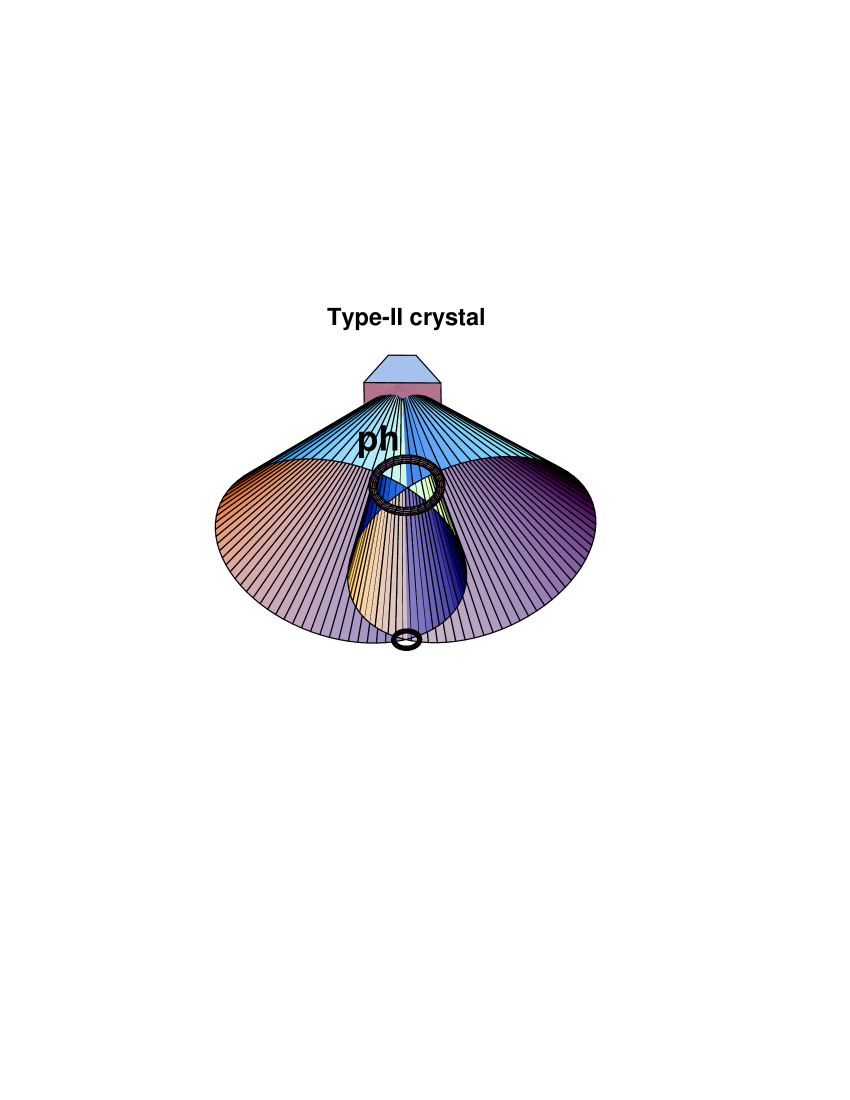
Figure 2: Photons from the cones are mutually perpendicularly polarized and therefore the photons from the intersections of the cones are in a singlet–like state. We chose pinhole ph five times bigger than the other one (determined by detectors D1’ and D2’) so that for each photon which passed through the latter pinhole, its companion photon will pass through ph.

By an appropriate preparation one can entangle them in a singlet–like state. [15] Their state is therefore

$$|\Psi\rangle={1\over\sqrt{2}}\bigl{(}|1_{x}\rangle_{1}|1_{y}\rangle_{1^{\prime}}\>-\>\,|1_{y}\rangle_{1}|1_{x}\rangle_{1^{\prime}}\bigr{)}\otimes{1\over\sqrt{2}}\bigl{(}|1_{x}\rangle_{2}|1_{y}\rangle_{2^{\prime}}\>-\>\,|1_{y}\rangle_{2}|1_{x}\rangle_{2^{\prime}}\bigr{)}\,.$$ (4)

The outgoing electric–field operators describing photons which pass through beam splitter BS and through polarizers P1’ and P2’ (oriented at angles $\theta_{1^{\prime}}$ and $\theta_{2^{\prime}}$, respectively) and are detected by detectors D1’ and D2’ will thus read (see Fig. 3)

$$\hat{E}_{1^{\prime}} = \left(\hat{a}_{1^{\prime}x}t_{x}\cos\theta_{1^{\prime}}+\hat{a}_{1^{\prime}y}t_{y}\sin\theta_{1^{\prime}}\right)e^{i{\mathbfit k}_{1^{\prime}}\cdot{\mathbfit r}_{1^{\prime}}-i\omega_{1^{\prime}}(t-t_{1^{\prime}}-\tau_{1^{\prime}})}$$ (5)

$$+\ i\left(\hat{a}_{2^{\prime}x}r_{x}\cos\theta_{1^{\prime}}+\hat{a}_{2^{\prime}y}r_{y}\sin\theta_{1^{\prime}}\right)e^{i\tilde{\mathbfit k}_{2^{\prime}}\cdot{\mathbfit r}_{1^{\prime}}-i\omega_{2^{\prime}}(t-t_{2^{\prime}}-\tau_{1^{\prime}})}\,,$$

where $t_{x}^{2}$, $t_{y}^{2}$ are transmittances, $r_{x}^{2}$, $r_{y}^{2}$ are reflectances, $t_{j}$ is time delay after which photon $j$ reaches BS, $\tau_{1^{\prime}}$ is time delay between BS and D1’, and $\omega_{j}$ is the frequency of photon $j$. The annihilation operators act as follows: ${\hat{a}}_{1x}|1_{x}\rangle_{1^{\prime}}=|0_{x}\rangle_{1^{\prime}}$,  ${\hat{a}}_{1x}|0_{x}\rangle_{1^{\prime}}=0$. $E_{2^{\prime}}$ is defined analogously. Operators describing photons which pass through polarizers P1 and P2 (oriented at angles $\theta_{1}$ and $\theta_{2}$, respectively), and through Pockels cells and are detected by detectors D1 and D2 will thus read

$$\hat{E}_{1}=(\hat{a}_{1x}\cos\theta_{1}+\hat{a}_{1y}\sin\theta_{1})e^{-i\omega_{1}t_{1}}\,.$$ (6)

$E_{2}$ is defined analogously.

Figure 3: Beam splitter BS detail from Fig. 1.

The probability of detecting all four photons by detectors D1, D2, D1’, and D2’ is thus

$$P(\theta_{1^{\prime}},\theta_{2^{\prime}},\theta_{1},\theta_{2}) = \eta^{2}\langle\Psi|\hat{E}_{2^{\prime}}^{\dagger}\hat{E}_{1^{\prime}}^{\dagger}\hat{E}_{2}^{\dagger}\hat{E}_{1}^{\dagger}\hat{E}_{1}^{\phantom{\dagger}}\hat{E}_{2}^{\phantom{\dagger}}\hat{E}_{1^{\prime}}^{\phantom{\dagger}}\hat{E}_{2^{\prime}}^{\phantom{\dagger}}|\Psi\rangle$$ (7)

$$= {\eta^{2}\over 4}(A^{2}+B^{2}-2AB\cos\phi)\,,$$

where $\eta$ is detection efficiency; $A=Q(t)_{11^{\prime}}Q(t)_{22^{\prime}}$ and $B=Q(r)_{12^{\prime}}Q(r)_{21^{\prime}}$; here $Q(q)_{ij}=q_{x}\sin\theta_{i}\cos\theta_{j}-q_{y}\cos\theta_{i}\sin\theta_{j}$; $\phi=(\tilde{\mbox{\boldmath$k$}}_{2}-\mbox{\boldmath$k$}_{1})\cdot\mbox{\boldmath$r$}_{1}+(\tilde{\mbox{\boldmath$k$}}_{1}-\mbox{\boldmath$k$}_{2})\cdot\mbox{\boldmath$r$}_{2}=2\pi(z_{2}-z_{1})/L$; here $L$ is the spacing of the interference fringes (see Fig. 3). $\phi$ can be changed by moving the detectors transversally to the incident beams. Data for this expression are collected by detectors D1’ and D2’ whose openings are not points but have a certain width $\Delta z$. Therefore, in order to obtain a realistic probability we integrate Eq. (7) over $z_{1}$ and $z_{2}$ over $\Delta z$ to obtain

$$P(\theta_{1^{\prime}},\theta_{2^{\prime}},\theta_{1},\theta_{2}) = {\eta^{2}\over 4}\int\limits_{z_{1}-{\Delta z\over 2}}\limits^{z_{1}+{\Delta z\over 2}}\int\limits_{z_{2}-{\Delta z\over 2}}\limits^{z_{2}+{\Delta z\over 2}}\Bigl{[}A^{2}+B^{2}-2AB\cos\bigl{[}{2\pi(z_{2}-z_{1})\over L}\bigr{]}\Bigr{]}dz_{1}dz_{2}$$ (8)

$$= {\eta^{2}\over 4}(A^{2}+B^{2}-v2AB\cos\phi)\,,$$

where $v=\bigl{[}\sin(\pi\Delta z/L)/(\pi\Delta z/L)\bigr{]}^{2}$ is the visibility of the coincidence counting. We assume the near normal incidence at BS so as to have $r_{x}^{2}=r_{y}^{2}=R$ and $t_{x}^{2}=t_{y}^{2}=T=1-R$. Next we assume a symmetric position of detectors D1’ and D2’ with respect to BS and the photons paths from the middle of the crystals so as to obtain $\phi=0$. [17,21] Representing photons by a Gaussian amplitude distribution of energies we have shown in Ref. [21] that the visibility is reduced when the condition $\omega_{1^{\prime}}=\omega_{2^{\prime}}$ is not perfectly matched and when the coincidence detection time is not much smaller than the coherence time. We meet the latter demand by using a subpicosecond laser pump beam and the former by reducing the size of the detector (D1’ and D2’) pinholes. By reducing the size of the detector pinholes we reduce the number of events detected by D1 and D2 but, on the other hand, this enables us to increase visibility of the Bell pairs at D1 and D2 by sizing pinholes $ph$ (see Fig. 2) so as to make solid angles five times wider than the pinholes of D1’ and D2’. (Cf. Joobeur, Saleh, and Teich. [13]) Alternatively, we can put $\omega_{0}/2$ filters ($\omega_{0}$ is the frequency of the pumping beam) in front of detectors D1 and D2 and drop the pinholes $ph$ altogether.

Let us now see in which way and when are all photons entangled. For $R=T=1/2$ and $v=1$ the probability Eq. (8) reads as

$$P(\theta_{1^{\prime}},\theta_{2^{\prime}},\theta_{1},\theta_{2})={1\over 4}(A-B)^{2}={1\over 16}\sin^{2}(\theta_{1^{\prime}}-\theta_{2^{\prime}})\sin^{2}(\theta_{1}-\theta_{2})\,.$$ (9)

and if we take away polarizers P1’ and P2’ the following maximal entanglement survives: $P(\infty^{\prime},\infty^{\prime},\theta_{1},\theta_{2})={1\over 8}\sin^{2}(\theta_{1}-\theta_{2})$. For an asymmetrical BS, however, if we take away polarizers P1’ and P2’, we obtain only partially entangled state

$$P(\infty^{\prime},\infty^{\prime},\theta_{1},\theta_{2})={1\over 4}[(T-R)^{2}+2TR\sin^{2}(\theta_{1}-\theta_{2})]\,.$$ (10)

Thus, in order to obtain (non)maximal entangled state for an asymmetrical beam splitter it is necessary to orient polarizers P1’ and P2’ so as to obtain a corresponding “entangled” probability given by Eq. (7). For example, for $\phi=0^{\circ}$, $\theta_{1^{\prime}}=90^{\circ}$, and $\theta_{2^{\prime}}=0^{\circ}$, Eq. (7) projects out the following (non)maximal singlet–like probability:

$$P(\theta_{1},\theta_{2}) = \eta^{2}s(\cos^{2}\theta_{1}\sin^{2}\theta_{2}-2v\rho\cos\theta_{1}\sin{\theta_{1}}\cos\theta_{2}\sin{\theta_{2}}+\rho^{2}\cos^{2}\theta_{2}\sin^{2}\theta_{1})$$ (11)

$$\equiv \eta^{2}p(\theta_{1},\theta_{2})$$

where $s=T^{2}/(R^{2}+T^{2})$, $\rho=R/T$, and where we multiplied Eq. (8) by 4 for other three possible coincidence detections [($\theta_{1^{\prime}}^{\phantom{\perp}}$,$\theta_{2^{\prime}}^{\perp}$), ($\theta_{1^{\prime}}^{\perp}$,$\theta_{2^{\prime}}^{\phantom{\perp}}$), and ($\theta_{1^{\prime}}^{\perp}$,$\theta_{2^{\prime}}^{\perp}$)] at BS and by $(R^{2}+T^{2})^{-1}$ for photons emerging from the same side of BS.

The singles–probability of detecting a photon by D1 is

$$P(\theta_{1})=\eta s(\cos^{2}\theta_{1}+\rho^{2}\sin^{2}\theta_{1})\equiv\eta p(\theta_{1})\,.$$ (12)

Analogously, the singles–probability of detecting a photon by D2 is

$$P(\theta_{2})=\eta s(\sin^{2}\theta_{2}+\rho^{2}\cos^{2}\theta_{2})\equiv\eta p(\theta_{2})\,.\hfill$$ (13)

Introducing the above obtained probabilities into the Clauser–Horne inequality (2) we obtain the following minimal efficiency for its violation.

$$\eta={p(\theta_{1}^{\prime})-p(\theta_{2})\over p(\theta_{1},\theta_{2})-p(\theta_{1},\theta_{2}^{\prime})+p(\theta_{1}^{\prime},\theta_{2}^{\prime})+p(\theta_{1}^{\prime},\theta_{2})}\,.\hfill$$ (14)

This efficiency is a function of visibility $v$ and by looking at Eqs. (11), (12), and (13) we see that for each particular $v$ a different set of angles should minimize it.

A computer optimization of angles—presented in Fig. 4—shows that the lower the reflectivity is, the lower is the minimal detection efficiency. Also, we see a rather unexpected property that a low visibility does not have a significant impact on the violation of the Bell inequality. For example, with 70% visibility and 0.2 reflectivity of the beam splitter we obtain a violation with a lower detection efficiency than with 100% visibility and 0.5 ($\rho=1$) reflectivity.

A similar calculation can be carried out for the Hardy equalities given at the and of Sec. 2. It can be shown that the lowest possible $R$, with only 5–10 standard deviations, should be taken and not the one which gives the greatest $P(\theta_{1},\theta_{2})>0$, again because the impact of a low visibility is the lowest when the beam splitter is the most asymmetrical. Thus our preselection scheme can be used for a loophole–free “Hardy experiment” as well.

Figure 4: Minimal detection efficiencies $\eta$ necessary for a violation of the Bell–Clauser–Horne inequality as functions of visibility $v$ and of $\rho=R/(1-R)$, where $R$ is the reflectivity of the beam splitter.

4 Conclusion

Our elaboration shows that the recently found four–photon entanglement [18,21] can be used for a realization of loophole–free Bell experiments. We propose a set–up which uses two simultaneous type–II downconversions into two singlet–like photon pairs. By combining two photons, one from each such singlet–like pair, at an asymmetrical beam splitter and detecting them in coincidence we preselect the other two completely independent photons into another singlet–like state—let us call them ‘Bell pair’. (See Figs. 1 and 3.) Our calculations show that no time or space windows are imposed on the Bell pairs by the preselection procedure and this means that we can collect the photons within an optimal solid angle. If we take their solid angles five times wider than the angles of preselector photons (determined by the openings of detectors D1’ and D2’—see Fig. 1), then we can collect all Bell pairs and at the same time keep a probability of the “third party” counts negligible.

For our set–up we can use the result presented in Fig. 4 which enables a conclusive violation of Bell’s inequalities with a detection efficiency lower than 80% even when the visibility is under 70% at the same time. If we, however, agree that it is physically plausible to take into account only those Bell pairs which are preselected by actually recorded detections at the beam splitter (firing of D1’ and D2’), then we can eliminate the low visibility impact altogether. In this case, we can set $v=1$ and for a different set of angles obtain a conclusive violation of Bell’s inequalities and Hardy’s equalities with still lower (under 70%) detection efficiency.

In the end, we stress that the whole device can also be used for delivering ready–made Bell pairs in quantum cryptography and quantum computation and communication.

Acknowledgments

I acknowledge supports of the Alexander von Humboldt Foundation, and the Ministry of Science of Croatia.

References

 [1] Ardehali, M., Phys. Rev. A 49, R3143 (1994).

 [2] Ardehali, M., Phys. Rev. A 49, R3143 (1994).

 [3] Clauser, J. F. and M. A. Horne, Phys. Rev. D 10, 526 (1974).

 [4] Clauser, J. F. and A. Shimony, Rep. Prog. Phys. 41, 1881 (1978).

 [5] Eberhard, P. H., Phys. Rev. A, 47, R747 (1993).

 [6] Fry, E. S., T. Walther, and S. Li, Phys. Rev. A 52, 4381 (1995).

 [7] Garg, A. and N. D. Mermin, Phys. Rev. D 35, 3831 (1987).

 [8] Garuccio, A., Ann. N. Y. Acad. Sci. 755 632 (1995).

 [9] Hardy, L., Phys. Rev. Lett. 71, 1665 (1993).

[10] Home, D. and F. Selleri, Riv. Nuovo Cim. 14, No. 9, (1991).

[11] Huelga, S. F., M. Ferrero, and E. Santos, Phys. Rev. A 51, 5008 (1995).

[12] Jones, R. T. and E. G. Adelberger, Phys. Rev. Lett. 72, 267 (1994).

[13] Joobeur, A., B. E. A. Saleh, and M. C. Teich Phys. Rev. A 50, 3349 (1994).

[14] Kwiat, P. G., P. H. Eberhard, A. M. Steinberg, and R. Y. Chiao, Phys. Rev. A, 49, 3209 (1994).

[15] Kwiat, P. G. , K. Mattle, H. Weinfurter, and A. Zeilinger, Phys. Rev. Lett.  75, 4337 (1995).

[16] Ou, Z. Y. and L. Mandel, Phys. Rev. Lett. 61, 50 (1988);

[17] Pavičić, M., Phys. Rev. A 50, 3486 (1994).

[18] Pavičić, M., J. Opt. Soc. Am. B, 12, 821 (1995).

[19] Pavičić, M., Phys. Lett. A 209, 255 (1995).

[20] Pavičić, M. in Fourth International Conference on Squeezed States and Uncertainty Relations, (NASA CP 3322, Washington, 1996), pp. 325.

[21] Pavičić, M. and J. Summhammer, Phys. Rev. Lett. 73, 3191 (1994).

[22] Santos, E., Phys. Rev. Lett. 66, 1388 (1991).

[23] Santos, E., Phys. Rev. Lett. 68, 2702 (1992).

[24] Santos, E., Phys. Rev. A 46, 3646 (1992).

[25] Santos, E., Phys. Lett. A 212, 10 (1996).

[26] Torgerson, J., D. Branning, and L. Mandel, App. Phys. 60, 267 (1995).

[27] Torgerson, J., D. Branning, C.H. Monken, and L. Mandel, Phys. Lett. A 204, 323 (1995).