Approximate real time visualization of a Rabi transition by means of continuous fuzzy measurement

Abstract

Continuous weak or fuzzy measurement of the Rabi oscillation of a two level atom subjected to a $\pi-$pulse of a resonant light field is simulated numerically. We thereby address the question whether it is possible to measure characteristic features of the motion of the state of a single quantum system in real time. We compare two schemes of continuous measurement: continuous measurement with constant fuzziness and with fuzziness changing in the course of the measurement. Because the sensitivity of the Rabi atom to the influence of the measurement depends on the state of the atom, it is possible to optimize the continuous fuzzy measurement by varying its fuzziness.

1 Introduction

We consider a single two-level atom with energy eigenstates $|E_{1}\rangle$ and $|E_{2}\rangle$ under the influence of a time dependent potential $V(t)$. Assuming $V(t)$ is not known and the evolution of the atom in the potential can be observed only once, which scheme of measurement conveys the most information about the otherwise undisturbed motion of the state $|\psi(t)\rangle$ of the atom in the potential? We will restrict to a reduced information and ask how to optimally record with minimal disturbance the evolution in time of the squared modulus of one of the components of the state of the atom, say $|c_{2}(t)|^{2}$, where $|\psi(t)\rangle=c_{1}(t)|E_{1}\rangle+c_{2}(t)|E_{2}\rangle$ is the normalized state vector. What types of measurement are to our disposition?
In order to detect the evolution of $|c_{2}(t)|^{2}$ by means of projection measurements of energy, the system has to be prepared new before each measurement in the same initial state with the same potential $V(t)$. If a sequence of consecutive projection measurements is applied because the system cannot be prepared new, the dynamics of the atom are in general strongly altered [1]. In the continuum limit of an infinite sequence of projection measurements the evolution can even be halted (Quantum Zeno effect) [2]. Therefore the usual projection measurements are not an appropriate choice to detect characteristic features of the evolution of the atomic state in real-time (i.e. without resetting the system).

In fact for this purpose two requirements have to be fulfilled simultaneously: the influence of the measurement on the dynamics of the system must not be too strong and the measurement readout has to be accurate enough to indicate the evolution of the state. The difficulty lies in the unavoidable competition of these properties: the better the dynamics are conserved (i.e. the smaller the influence of the measurement), the less reliable is the readout and vice versa.

We will show below that an approach to a real-time visualization can profitably be based on unsharp measurements which for example can be described in the POVM formalism [3]. Unsharp measurements are there associated with observables that can not be represented as projection valued measures but only as positive operator valued measures. These measurements have the advantage that their influence is less strong than the influence of projection measurements, but at the same time they have a lower resolution. In order to obtain information about $|c_{2}(t)|^{2}$ in real-time, if only one realization of the evolution is available, a whole sequence of unsharp measurements is required. For calculational convenience we consider such sequences in the limit of continuous measurements.

A continuous measurement of energy lasts over a certain time period ($0\leq t\leq T$) and produces a readout denoted by $[E]=\{(t,E(t))|0\leq t\leq T\}$ which assigns to each time $t$ during this period a measured value $E(t)$. It serves to detect the evolution of a quantum mechanical system. Continuous measurements have been investigated in several contexts [4]. Since we use unsharp measurements the readout possesses in general a low accuracy and shows quantum fluctuations. Therefore these measurements are called continuous fuzzy measurements. We will base our considerations below on a phenomenological model, which also makes plausible that a correlation between $E(t)$ and $|c_{2}(t)|^{2}$ is to be expected. For a realization scheme see [5].

With continuous fuzzy measurements we have found a possible candidate for the measurement scheme with the desired properties. But note, that according to the nature of quantum mechanics, there is no scheme that precisely records the evolution of $|c_{2}(t)|^{2}$ in real-time without influencing it as well. All we can do is to find a mechanism, that allows a “best bet” on the behaviour of $|c_{2}(t)|^{2}$, if only one “run” is available.

The relation between the modification of the motion of the state and the reliability of a readout has been investigated in [5, 6, 7]. There it was shown for measurements with constant fuzziness, that a visualization can be achieved up to a certain degree if the value of fuzziness is properly chosen. In the present work we want to extend the investigation to the case where the parameter which determines the fuzziness of the measurement is varied as function of time or is made dependent on the readout $E(t)$ of the measurement. Our intention is to show that in this way it is possible to improve the efficiency of the visualization achieved with constant fuzziness.

A restrictive remark has to be made. We will not try to answer the question posed initially in full generality. Instead of the unknown driving potential $V(t)$ we will consider the special case of the atom being subject to a $\pi-$ pulse of a resonant light field. Being initially in the ground state $|E_{1}\rangle$, the atom — in the absence of any measurement — carries out a transition to the upper state $|E_{2}\rangle$ (Rabi transition). This is the undisturbed motion to be visualized by means of our measurement scheme. The evaluation of continuous fuzzy measurements is done by Monte Carlo simulations. From the results obtained here we get insights for the more general case of an unknown $V(t)$.

The paper is organized as follows: Section 2 contains a brief description of the phenomenological model used to describe continuous fuzzy measurements. In section 3 we define quantities that represent the modification of the dynamics due to the influence of the measurement on one hand and the reliability of the readouts on the other. These quantities are then evaluated for measurements with constant fuzziness. In section 4 we investigate continuous measurements with time dependent fuzziness. In section 5 continuous measurements with fuzziness depending on the readout are studied. Both are compared with the measurements with constant fuzziness. The scheme of measurement introduced in section 5 can also be used in the general case of unknown dynamics. We conclude with a summary in section 6.

2 Continuous fuzzy measurements

We consider a two level atom submitted to a $\pi$-pulse of intensive, resonant laser light. The respective Hamiltonian reads

$$H=E_{1}|E_{1}\rangle\langle E_{1}|+E_{2}|E_{2}\rangle\langle E_{2}|+v_{0}\left(\exp\{-i\omega(t\}|E_{2}\rangle\langle E_{1}|+h.c.\right)\,,$$ (1)

with $\omega=(E_{2}-E_{1})/\hbar$ and $v_{0}=\langle E_{2}|{\mathbf{d}}{\mathbf{E}}|E_{1}\rangle$, where ${\mathbf{d}}$ is the dipole moment of the atom and ${\mathbf{E}}$ is the amplitude of the electric field strength. The pulse lasts from $t=T_{1}$ untill $t=T_{2}$. If no further influence is present, an atom in the ground state at $t=T_{1}$ performs a Rabi transition to the upper state $|E_{2}\rangle$ in the course of the $\pi$-pulse ($T_{2}-T_{1}=\hbar\pi/v_{0}$). Before and after the pulse the dynamics of the atom is governed by its free Hamiltonian

$$H_{0}=E_{1}|E_{1}\rangle\langle E_{1}|+E_{2}|E_{2}\rangle\langle E_{2}|\,.$$ (2)

A continuous fuzzy measurement of energy (observable $H_{0}$) during the time interval $[0,T]$ containing $[T_{1},T_{2}]$ produces a readout $[E]$.

Since we want to discuss a measurement applied to a single atom we employ in the following a selective description of the measurement. Given the initial state of the atom and given a particular readout $[E]$, a theory describing continuous fuzzy measurements has to answer the following two questions: i) how has the state evolved during the measurement and ii) what is the probability density $p[E]$ to measure the readout $[E]$. The answers can be given in a phenomenological theory of continuous measurements. For a survey of this theory see [8]. As already mentioned in the introduction, these measurements find their realization by means of sequences of unsharp measurements [5].

Given a certain readout $[E]$, the effective Schrödinger equation

$$i\hbar\frac{\partial}{\partial t}|\psi^{[E]}_{t}\rangle=H_{[E]}|\psi^{[E]}_{t}\rangle$$ (3)

with complex Hamiltonian $H_{[E]}$

$$H_{[E]}\ =H-i\kappa\hbar\,\big{(}H_{0}-E(t)\big{)}^{2}$$ (4)

determines the unnormalized solution $|\psi^{[E]}_{t}\rangle$, thus giving the answer to question i). From this the probability density in question ii) can be evaluated by

$$p\left[E\right]=\langle\psi_{T}^{[E]}|\psi_{T}^{[E]}\rangle\,\$$ (5)

The second term in the Hamiltonian (4) leads to damping of the amplitude of $|\psi_{t}^{[E]}\rangle$. The amount of damping for fixed $\kappa$ depends on how close the readout $[E]$ is to the curve of the expectation value $\langle H_{0}\rangle$, for details see [6]. Large damping implies because of (5), that the readout is improbable. In (4) $\kappa$ represents the strength of the measurement. If $\kappa$ is small, such that $H$ dominates $H_{[E]}$, the measurement perturbs the evolution only a little. If $\kappa$ is great, the evolution is overwhelmed by the influence of the measurement.

The influence of the fuzzy measurement on the atom competes with the influence of the external field driving the atom to the upper level. The strength of the latter is characterized by half the Rabi period $T_{R}/2$ - the time a Rabi transition takes without measurement. In order to compare both influences, we introduce a characteristic time for the continuous measurement [6]. The effective resolution time

$$T_{\mathrm{e}ff}:=\frac{4\pi}{\kappa\Delta E^{2}}\,,$$ (6)

may serve as a measure of fuzziness of a continuous measurement. In what follows we refer to this quantity simply as fuzziness $T_{\mathrm{e}ff}$.

3 Efficiency of visualization

As already pointed out in the introduction, the visualization of a single Rabi transition by a continuous measurement becomes efficient if two properties are fulfilled : weak influence (later on specified as softness) of the measurement and reliability of the measurement readouts. In this section we first introduce quantities to specify these properties and then apply them to characterize measurements with constant fuzziness.

3.1 Softness and Reliability

For a visualization the measurement should be likely to only modify and not prevent the Rabi transition. In order to fix what can be regarded as a modified or approximate Rabi transition, we use the following, somewhat minimal condition:

$$|c_{2}(T)|^{2}>0.5$$ (7)

for the component

$$c_{2}(T)=\frac{|\langle E_{2}|\psi_{T}^{[E]}\rangle|^{2}}{\sqrt{\langle\psi_{T}^{[E]}|\psi_{T}^{[E]}\rangle}}\geq 0.5\,.$$ (8)

The probability that the state will perform such an approximate Rabi transition is given by

$$s:=\int_{\cal U}p[E]d[E]\;\;\;\mbox{with}\;{\cal U}=\{[E]\mid|c_{2}(T)|^{2}\geq 0.5\}\;.$$ (9)

We refer to $s$ as softness of the continuous measurement.

What can we read off from a readout [E] and how reliable is it? In order to answer these questions we turn to the realization given in [5] of the phenomenological scheme we are using. There it has been shown: if many single weak measurements of energy are performed on the same normalized states $|\psi(t_{0})\rangle$, then the statistical mean value $\tilde{E}(t_{0})$ of all individual measurement results $E$ obeys the relation

$$\frac{\tilde{E}(t_{0})-E_{1}}{\Delta E}=\frac{\bar{E}(t_{0})-E_{1}}{\Delta E}=|c_{2}(t_{0})|^{2}$$ (10)

with $\bar{E}(t_{0})=\langle\psi(t_{0})|H_{0}|\psi(t_{0})\rangle$. This has led to the idea to take $(E(t)-E_{1})/\Delta E$ of a complete single readout $[E]$ obtained under the influence of the driving potential as an estimate of $|c_{2}(t)|^{2}$. How reliable is this?

Turning again to the total curves we introduce a mean deviation $d$ according to

$$d^{2}=\int p[E]d[E]\frac{1}{T}\int dt\left[\frac{E(t)-E_{1}}{\Delta E}-|c_{2}(t)|^{2}\right]^{2}\;.$$ (11)

We call $r=1/d$ the reliability of a continuous measurement. It indicates how reliable it is, that $(E(t)-E_{1})/\Delta E$ of a single readout agrees with $|c_{2}(t)|^{2}$.

3.2 Constant fuzziness

We apply the concepts introduced in section 3.1 to the special case of measurements with fuzziness $T_{\mathrm{e}ff}$ kept constant during the measurement (comp. [5, 6, 7]). The numerically obtained results are displayed in Fig. 1 and Fig. 3.

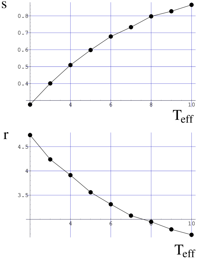
Figure 1: Upper part: softness $s$ of the influence of a continuous measurement for different values of constant fuzziness $T_{\mathrm{e}ff}$ (in units of $T_{R}/3$). Lower part: The correspondent reliability $r$ of a readout regarding the question whether it represents the evolution of $|c_{2}(t)|^{2}$

Fig. 1 shows, how with growing fuzziness $T_{\mathrm{e}ff}$ softness $s$ increases and reliability $r$ decreases. For low fuzziness we see the Zeno regime of strong measurement. The state motion differs largely from the Rabi transition, but is well visualized. In the Rabi regime of high fuzziness the Rabi transition of the state is preserved but cannot be visualized by the readout. The relation between reliability and softness for measurements with constant fuzziness can be seen from Fig 3 (small circles). The pairs $(r,s)$ for different values of fuzziness lie almost on a straight line.

Returning to our initial question we study a continuous measurement in the intermediate regime. For $T_{\mathrm{e}ff}=5$ an approximate transition takes place in $60$ percent of the cases ($s=0.6$) and the mean deviation amounts to $d=0.28$ in units of $\Delta E$. For a single measurement it is therefore to be expected that the readout $[E]$ reflects approximately the evolution of $|c_{2}|^{2}$.

We now address the question whether an improvement of $r$ and $s$ can be achieved if fuzziness varies in the course of the measurement.

4 Time dependent fuzziness

In order to improve the efficiency of the continuous fuzzy measurement one may for example think of choosing a low fuzziness $T_{\mathrm{e}ff}$. This increases the reliability $r$ but decreases softness $s$. If fuzziness $T_{\mathrm{e}ff}$ is kept low over the whole measurement not much is gained because the original Rabi transition is strongly modified. But there are specific time intervals at which even a strong influence of an energy measurement (small softness) is likely to modify a Rabi transition only to a small amount. This is at the beginning ($t=T_{1}$) and at the end ($t=T_{2}$) of the $\pi$-pulse when the state of the undisturbed Rabi transition is close to an energy eigenstate. Even a projection measurement is not likely to modify the state very much in this case. Just the opposite situation can be found in the middle of a $\pi$-pulse. Both observations lead to the idea to vary fuzziness in time in order to take advantage of the varying sensitivity of the system. In order to do so, one has to know the time development of the state $|\psi(t)\rangle$ beforehand, accordingly $V(t)$ must be known . We discuss as above the real-time visualization of a Rabi transition.

We assume a time dependent fuzziness $T_{\mathrm{e}ff}(t)$ of Gaussian shape (comp. Fig. 2) with width $\delta T$. The maximum $T_{\mathrm{e}ff}^{\mathrm{(}m)}$ is located at the middle of the pulse at $t=(T_{1}+T_{2})/2$. An offset value $T_{\mathrm{e}ff}^{(0)}\neq 0$ is obtained at $t=0$ and $t=T$. In order to see the influence of a varying width $\delta T$, the maximum $T_{\mathrm{e}ff}^{\mathrm{(}m)}$ and the minimum $T_{\mathrm{e}ff}^{(0)}$ are kept fixed and the Gaussian is rescaled appropriately. This leads to

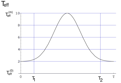
Figure 2: Time dependent fuzziness $T_{\mathrm{e}ff}$ (in units of $T_{R}/3$) with width $\delta T=0.2$.

$$T_{\mathrm{e}ff}(t)=a\lambda(t)+b$$ (12)

with

$$\lambda(t):=\exp\left(\frac{(t-T/2)^{2}}{2(\delta T)^{2}}\right)\;$$ (13)

and

$$a:=\frac{T_{\mathrm{e}ff}^{(m)}-T_{\mathrm{e}ff}^{(0)}}{1-\lambda(T)}\;,\;\;b=:T_{\mathrm{e}ff}^{(m)}-a\,.$$ (14)

We computed the reliability $r$ and softness $s$ of measurements with fuzziness $T_{\mathrm{e}ff}(t)$ for different width $\delta T$. The results can be seen in Fig. 3 where pairs of $(r,s)$ are plotted for time dependent fuzziness (small squares) and constant fuzziness (small circles). We consider a measurement characterized by $(r^{(1)},s^{(1)})$ to be “better than” a measurement with $(r^{(2)},s^{(2)})$ if both — the reliability and the softness of the first measurement — are greater: $s^{(1)}>s^{(2)}$ and $r^{(1)}>r^{(2)}$. In fact not all measurements are comparable in terms of this definition but the ones which are better than a particular one lie in the diagram on the right and higher. The ones worse than the particular one lie to the left and lower. The best measurement of the diagram would lie in its upper right corner.

Fig. 3 shows that the results of measurements with constant fuzziness can clearly be improved by using measurements with time dependent fuzziness. For example the measurement with time dependent fuzziness and width $\delta T=0.2$ is better than measurements with constant fuzziness with $4.3\leq T_{\mathrm{e}ff}\leq 6$. The former measurement leads to $s=69\%$ and $d=0.26\Delta E$.

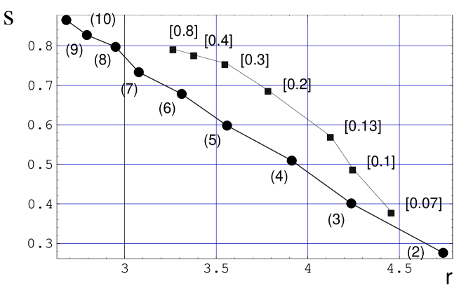
Figure 3: Comparison between constant fuzziness ( small circles , the number in round brackets is to value of $T_{\mathrm{e}ff}$) and time dependent fuzziness (small squares, number in straight brackets is the width $\delta T$ in units of $T_{\rm R}/2$, $T_{\mathrm{e}ff}^{\mathrm{(}m)}=10,T_{\mathrm{e}ff}^{(0)}=2$). $s$ is the softness of a measurement and $r$ its reliability.

Another way to display the results of the numerical calculations are density plots of the readouts $[E]$ and the curve of the squared component $|c_{2}(t)|^{2}$. The density plot of the readouts $[E]$ is obtained by dividing the E-t-plane into squares of equal area and calculating the probability that a smoothed curve [E] (c.f. Appendix) crosses a particular square.

$$P_{S}:=\int_{S}P[E]d[E]\;,\mbox{with}\;\;S=\{[E]|(t,E(t))\in\mbox{square}\}\;.$$ (15)

The degree of grayness of the square is then chosen according to $P_{S}$. The $|c_{2}(t)|^{2}$-density plot is created analogously, apart from the fact that the curves $|c_{2}(t)|^{2}$ do not have to be smoothed, since they do not posses rapid oscillations.

In Fig. 4 density plots for constant fuzziness and for time dependent fuzziness are displayed. The latter shows an improved correlation between readout $[E]$ and squared component $|c_{2}(t)|^{2}$. In particular we can read off from the energy plots that the area with the second smallest degree of grayness (corresponding to $0.3\leq P_{S}\leq 0.4$) is more narrow for time dependent fuzziness than for constant fuzziness. While in case of constant fuzziness there are still two branches of readouts (going up and staying down), for time dependent fuzziness there is only one strong branch representing curves that show an approximate transition. The plots of the squared component $|c_{2}(t)|^{2}$ indicate a greater softness for measurements with time dependent fuzziness. Both kinds of measurements show two branches, for time dependent fuzziness the ends of both branches are more narrow than for constant fuzziness.

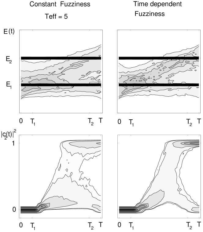
Figure 4: Visibility of the atomic transition: on the left with constant fuzziness ($T_{\mathrm{e}ff}=5$), on the right with time dependent fuzziness $T_{\mathrm{e}ff}(t)$ ($\delta T=0.2$). The upper diagrams show density plots of measured energy curves (measured energy versus time). The lower density plots display the corresponding curves of the squared component $|c_{2}(t)|^{2}$ over time $t$. Comparing constant with time dependent fuzziness, there is a progress in terms of visibility of the transitions.

5 Energy dependent fuzziness

In the general case the driving potential $V(t)$ and therefore the dynamics of the system without measurement are unknown. It will thus not be possible to design beforehand an adjusted time dependent fuzziness $T_{\mathrm{e}ff}(t)$. Nevertheless one can also in this case take advantage of varying fuzziness. Applying the same reasoning as for time dependent fuzziness, we have to use a large fuzziness (small perturbation by the measurement) when the system is not close to an energy eigenstate, i.e. for $|c_{2}(t)|^{2}\approx 1/2$. The value of the readout $E(t)$ is correlated to $|c_{2}(t)|^{2}$ and $\langle H_{0}\rangle_{t}$. This means that energy dependent fuzziness $T_{\mathrm{e}ff}(E)$ should have its maximum near $(E_{2}-E_{1})/2$ and should be low for $E_{1}$ and $E_{2}$.

We test this idea once more for the case of a driving potential which leads to a Rabi transition if no further influence is present. For $T_{\mathrm{e}ff}(E)$ we assume a Gaussian $T_{\mathrm{e}ff}(E)=a\lambda(E)+b$ with width $\delta E$ and

$$\lambda(E) := \exp\left(\frac{(E-(E_{2}+E_{1})/2)^{2}}{2(\delta E)^{2}}\right)\;,$$ (16)

$$a = \frac{T_{\mathrm{e}ff}^{(m)}-T_{\mathrm{e}ff}^{(0)}}{1-\lambda(E_{\mathrm{m}ax})}\;,\;\;b=T_{\mathrm{e}ff}^{(m)}-a\,.$$

We choose again as maximum $T_{\mathrm{e}ff}^{\mathrm{(}m)}=10$ and as minimum $T_{\mathrm{e}ff}^{(0)}=2$, comp. Fig. 5.

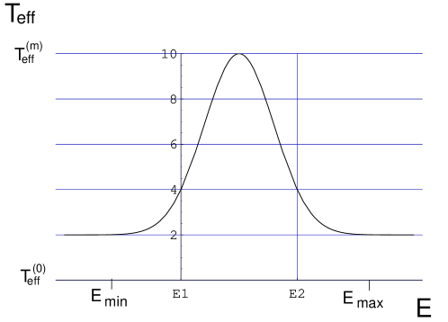
Figure 5: Energy dependent fuzziness $T_{\mathrm{e}ff}$ (in units of $T_{R}/3$) with width $\delta E=0.3$

.

The results in terms of reliability and softness for different values of $\delta E$ (small squares) are plotted in Fig. 6. They can be compared with the values of $r$ and $s$ from constant fuzziness. As in the case of time dependent fuzziness, there is no improvement of measurements with high or low constant fuzziness. But in the intermediate regime, which is the important one for visualization, the results for energy dependent fuzziness are better than for constant fuzziness. It is satisfying that in this regime not only with time dependent but also with energy dependent fuzziness the results from constant fuzziness can be improved. Time dependent fuzziness leads in the intermediate regime to slightly higher values of reliability and softness than energy dependent measurements.

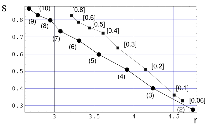
Figure 6: Comparison between constant fuzziness (small circles, the number in round brackets is the value of $T_{\mathrm{e}ff}$) and energy dependent fuzziness (small squares, the number in straight brackets is the width $\delta E$ in units of $\Delta E$, $T_{\mathrm{e}ff}^{\mathrm{(}m)}=10,T_{\mathrm{e}ff}^{(0)}=2$). $s$ is the softness of the measurement and $r$ its reliability.

6 Conclusion

The normalized state $|\psi(t)\rangle=c_{1}(t)|E_{1}\rangle+c_{2}(t)|E_{2}\rangle$ of a $2$-level atom performs Rabi oscillations under the influence of an external driving field. It is assumed that there is only one realization of this process. We ask the questions if it is possible to obtain a visualization of $|c_{2}(t)|^{2}$ in real-time using an appropriate measurement scheme. It is shown that this is possible up to a certain degree, if a continuous fuzzy measurement of energy is performed leading to a readout $[E]$. In order to quantify the efficiency of visualization for a given fuzziness we have introduced for a measurement the complementary concepts of softness (small disturbing influence) and reliability (the curve of $|c_{2}(t)|^{2}$ agrees essentially with the readout $[E]$). It is discussed in detail how both demands can be improved at the same time, if fuzziness is chosen to be appropriately time dependent or energy dependent.

7 Acknowledgment

This work has been supported in part by the Deutsche Forschungsgemeinschaft and the Optik Zentrum Konstanz.

Appendix: Numerical simulations

Numerical simulations

Since the effective Schrödinger equation (3) does not posses a closed form solution for general readout $[E]$, we simulated continuous fuzzy measurements numerically. The simulation can be divided into the following steps.

1. Generate a random curve $[E]$.

2. Insert $[E]$ into equation (3) and solve them with initial condition $|\psi_{0}\rangle=|E_{1}\rangle$.

3. Compute $p[E]$.

4. Repeat steps 1.-3. $n$ times and process data.

Description of the steps
Step 1.: Energy readouts are generated out of the class of functions

$$E(t)=g(t)+\sum_{k=1}^{m}\,a_{k}\sin\left(\frac{k\pi t}{T}\right)\,,$$ (17)

where $g(t)$ is a straight line. The initial and final value of the readout $E(0)=g(0)$ and $E(T)=g(T)$ are chosen by random out of the interval $I_{E}:=[E_{1}-\Delta E/2,E_{2}+\Delta E/2]$. In addition the Fourier coefficients $a_{k}$ are randomly taken out of $I_{a}:=[-0.35\Delta E,0.35\Delta E]$. In the simulations we used $m=10$, our results are stabile if higher Fourier terms are taken into account ($m>10$).
Step 2.: The effective Schrödinger equation is solved using computer algebra. The whole simulation was implemented in Mathematica [Wolfram Research]. In the computation of $|\psi_{t}^{[E]}\rangle$ we approximated $v(t)$ which describes the processes of turning on and turning off the laser by a product of two smoothed step functions.

Step 4.: Mean values of quantities $f$ that characterize a continuous measurement with a certain fuzziness are calculated from the data of the $n$ repetitions. They serve as approximation of the expectation value of f:

$$\bar{f}=\int f[E]p[E]d[E]\approx\frac{1}{N}\sum_{i=1}^{n}\;p[E_{i}]f[E_{i}]\quad\mbox{with}\,\,N=\sum_{i=1}^{n}\;p[E_{i}]\,.$$ (18)

We chose $n=10^{4}$ in order to obtain a relative error of $\delta\bar{f}/\bar{f}\approx 1\%$. $n$ has to be increased for larger intervals $I_{E},I_{a}$.
Density plots of the curves $|c_{2}(t)|^{2}$ and smoothed $[E]$ are made. $[E]$ is smoothed in order to extract information about the dynamics on the scale of the order of the Rabi period $T_{R}$. The smoothing is done by multiplying the Fourier coefficients $a_{k}$ with $exp\{-(k/3)^{2}\}$. Thereby fast oscillations are damped. A real measuring apparatus may not be able to display fast oscillations because of its inherent inertia.

References

- [1] M.J.Gagen and G.J.Milburn, Phys. Rev. A47, 1467, 1993.
- [2] B.Misra and E.C.G.Sudarshan, J. Math. Phys. 18, 756 (1977); C.B.Chiu, E.C.G. Sudarshan and B.Misra, Phys. Rev. D 16, 520 (1977); A.Peres, Amer. J. Phys. 48, 931 (1980); F.Ya.Khalili, Vestnik Mosk. Universiteta, ser. 3, no.5, p.13 (1988); W.M.Itano, D.J.Heinzen, J.J.Bollinger and D.J.Wineland, Phys. Rev. A 41, 2295 (1990); A.Beige and G.C.Hegerfeldt, Phys. Rev. A 53, 53 (1996).
- [3] S. Ali and G. Emch, J. Math. Phys. 15, 176 (1974); P. Bush, M. Grabowski, P. J. Lahti Operational Quantum Physics, Springer Verlag Heidelberg, 1995.
- [4] H.D.Zeh, Found. Phys. 1, 69 (1970); 3, 109 (1973); E. B. Davies, Quantum Theory of Open Systems, Academic Press: London, New York, San Francisco, 1976; M. D. Srinivas, J.Math. Phys. 18, 2138 (1977); A. Peres, Continuous monitoring of quantum systems, in Information Complexity and Control in Quantum Physics, ed. by A. Blaquiere, S. Diner, and G. Lochak, Springer, Wien, 1987, pp. 235; D. F. Walls and G. J. Milburn, Phys. Rev. A 31, 2403 (1985); E. Joos, and H. D. Zeh, Z.Phys. B 59, 223 (1985); L. Diosi, Phys. Lett. A 129, 419 (1988); H.Carmichael, An Open Systems Approach to Quantum Optics, Springer, Berlin and Heidelberg, 1993; A. Konetchnyi, M. B. Mensky and V. Namiot, Phys. Lett. A 177, 283 (1993); P.Goetsch and R .Graham, Phys. Rev. A 50, 5242 (1994); T.Steimle and G.Alber, Phys. Rev. A 53, 1982 (1996); M. B. Mensky, Phys. Rev. D 20, 384 (1979); Sov. Phys.-JETP 50, 667 (1979); M. B. Mensky, Continuous Quantum Measurements and Path Integrals, IOP Publishing: Bristol and Philadelphia, 1993; F.Ya.Khalili, Vestnik Moskovskogo Universiteta, ser. 3, v.29, no.5, p.13 (1988), in Russian; M. Brune, S. Haroche, V.Lefevre, J. M. Raimond, and N. Zagury, Phys. Rev. Lett. 65, 976 ((1990); Phys. Rev. A 45, 3260 (1992); V.B.Braginsky and F.Ya.Khalili, Quantum Measurement, ed. Kip S.Thorne, Cambridge University Press, Cambridge, 1992; N.Gisin, P.L.Knight, I.C.Percival and R.C.Thompson, J. Modern Optics 40, 1663 (1993); K.Jacobs and P.L.Knight, Phys. Rev. A 57, 2301 (1998); A. Peres, Quantum Theory: Concepts and Methods, Kluwer Academic Publishers, Dordrecht, Boston & London, 1993; R. Onofrio, C. Presilla, and U. Tambini, Phys. Lett. A 183, 135 (1993); U. Tambini, C. Presilla, R. Onofrio, Phys. Rev. A 51, 967 (1995).
- [5] J.Audretsch, M.Mensky “Realization scheme for continuous fuzzy measurement of energy and the monitoring of a quantum transition” Preprint: quant-ph/9808062
- [6] J.Audretsch and M.B.Mensky, Phys. Rev. A 56, 44 (1997).
- [7] J.Audretsch, M.Mensky and V.Namiot, Phys. Lett. A237, 1 (1997).
- [8] M. B. Mensky, Physics-Uspekhi, 41, 923, (1998).