Coherent two-field spectroscopy of degenerate two-level systems.

Abstract

Spectroscopic features revealing the coherent interaction of a degenerate two-level atomic system with two optical fields are examined. A model for the numerical calculation of the response of a degenerate two-level system to the action of an arbitrarily intense resonant pump field and a weak probe in the presence of a magnetic field is presented. The model is valid for arbitrary values of the total angular momentum of the lower and upper levels and for any choice of the polarizations of the optical waves. Closed and open degenerate two-level systems are considered. Predictions for probe absorption and dispersion, field generation by four-wave-mixing, population modulation and Zeeman optical pumping are derived. On all these observables, sub-natural-width coherence resonances are predicted and their spectroscopic features are discussed. Experimental spectra for probe absorption and excited state population modulation in the D₂ line of Rb vapor are presented in good agreement with the calculations.

I Introduction.

When an atomic transition is driven by quasi-resonant light, after a transient evolution, the quantum state describing the atomic system becomes correlated in time with the exciting light field. This correlation is in turn responsible for the coherent interaction between the atomic system and the light. Of special interest is the case when the atomic system interacts with two optical fields. In this case, in addition to the induced atomic coherence at the frequencies of the two fields, the non-linearity of the medium is responsible for atomic coherence at frequencies that result from the linear combinations of the frequencies of the two incident optical fields. These additional frequency components in the atomic dynamics manifest themselves in the spectral dependence of different observables such as absorption or new field generation.

The response of a pure two-level system, driven by a monochromatic pump wave and tested by a weak probe with variable frequency offset with respect to the pump, is well known [1, 2, 3]. In the case of a relatively weak pump field (Rabi frequency no larger than the transition natural width) the coherent interaction of the two-level system with the two fields is responsible for narrow features in probe absorption (occurring when the two-level transition is open) whose width is determined by the ground-state relaxation rate [4, 5]. Although theoretical predictions based in the simple two-level model have proven to be powerful for the interpretation of a large number of experimental results, pure two-level systems are seldom found in real experiments. In most cases, the atomic levels are degenerate and the vectorial nature of the electromagnetic field plays an essential role.

Well before the advent of the laser, it was realized that resonant light can modify the state of a degenerate atomic level through optical pumping among Zeeman sublevels[6]. Experiments using optical and/or radiofrequency excitation demonstrated the occurrence of orientation, alignment and Zeeman coherence. The invention of the laser opened the way to the study of the coherent response of degenerate system in the optical domain. Essential theoretical contributions in this subject are due to Berman and co-workers[7, 8, 9]. In their work, the crucial role of optical pumping in degenerate two-level system is underlined and it is demonstrated that sub-natural-width spectroscopic resonances are associated to the non conservation of population, orientation or alignment. The connection between these narrow spectroscopic features and sub-Doppler cooling was established in [8] and the pump-probe spectroscopy of degenerate two-levels systems including the effect of the atomic recoil was considered in [9]. Bo Gao[10, 11] has developed a method allowing the calculation of the weak probe absorption by a closed degenerate two-level system driven by a linearly polarized pump wave and no magnetic field. The resonance fluorescence spectrum of a driven degenerate two-level systems was qualitatively discussed with the help of the dressed atom model[12] and explicitly derived[13]. Also, let us mention that several authors have been concerned with the steady-state preparation of a degenerate two level system due to the excitation by a unique field of arbitrary elliptic polarization[14, 15, 10, 16, 17, 18].

In this paper we are concerned with the spectroscopic features of the coherent response of driven degenerate two level systems. Our attention is placed on the sub-natural-width resonances associated to the coherent nature of the interaction of an atomic system with a drive and a probe field. As discussed below, such resonances are present in a large variety of physical observables such as probe absorption, dispersion, fluorescence, four-wave-mixing (FWM) etc. The aim of this paper is to discuss the essential spectroscopic features of the coherence resonances present on these observables and discuss the dependence of these features in parameters such as external magnetic field, optical fields polarizations, light intensity and atomic level characteristics.

Additional motivation for the study of degenerate two-level systems arise from the connection of this problem with that of the study of multilevel configurations where interesting coherent effects have attracted considerable attention in recent years. Among them is the phenomenon of coherent population trapping (CPT)[19] and the related effect of electromagnetic induced transparency (EIT)[20] observed in three-level systems (mainly $\Lambda$ systems). These effects have found interesting application for subrecoil laser cooling[21], magnetometry[22], refractive index enhancement[23], enhancement of non-linear susceptibility[24], steep dispersion[25] and ultra-low group velocity propagation[26]. Degenerate two-level systems provide us with the possibility to analyze some of the level schemes studied so far within a unique theoretical frame. Under the appropriate choice of the pump and probe polarizations and the angular momenta of the involved levels, the degenerate two level system in the presence of two-fields reduces, as a particular case, into several of the multi-level configurations previously studied ($\Lambda,V,N$ configurations, etc.). One can thus expect that degenerate two level systems will be suitable for the observation of coherent effects including those previously predicted and observed in three level configurations. In addition, new effects such as Electromagnetically Induced Absorption (EIA)[27, 28] appear in the degenerate two level system that are not present in three-level configurations.

The first part of the paper is devoted to the presentation of a theoretical model allowing the calculation of the complete response to first order in the probe field of an atomic system composed of two degenerate levels of given total angular momentum driven by a pump wave. The model is based in a semiclassical treatment of the atom+fields dynamics based in optical Bloch equations[7, 8, 9, 10, 11]. It is intended to be suitable for the numerical calculation of the response of the atomic medium in a wide variety of cases: Arbitrary values of the total angular momentum of the ground and excited levels can be considered. Arbitrary and independent elliptical polarizations are allowed for the pump and probe waves. The presence of an external magnetic field is included. Both open and closed two-level systems can be treated.

The model results in the derivation of the equation 34 below satisfied by the operator $\sigma$ defined in order to contain all density matrix terms corresponding to the response of the atomic system (under the presence of the arbitrarily intense pump wave) to first order in the probe wave. Different spectroscopic observables such as probe absorption and dispersion, new field generation, population modulation, magnetic orientation, are subsequently derived from the operator $\sigma$ as discussed below. The spectral features present on these observables are then discussed with special attention on the subnatural-width resonances due to the coherent interaction between the atomic system and the fields. The predictions are illustrated with experimentally observations of probe absorption and fluorescence modulation carried on the D₂ lines of Rb vapor.

The paper is organized as follows. The second section is devoted to the presentation of the theoretical model and to the derivation of the expressions for different observables. The spectroscopic features of each of these observables as a function of the optical and magnetic field parameters are specifically discussed. The third section is devoted to experimental observations concerning probe absorption and population modulation spectra. Finally, some conclusions are presented.

II Theory.

A Model.

The model was developed having in mind transitions within the D lines of alkaline atoms. However, it is not restricted to this case. It can be applied to any dipole allowed atomic transition from a long-living lower level to an upper level rapidly damped by spontaneous emission. We consider two degenerate levels: a ground level $g$ of total angular momentum $F_{g}$ and energy $\hbar\omega_{g}$ and an excited state $e$ of angular momentum $F_{e}$ and energy $\hbar\omega_{e}$. The total radiative relaxation coefficient of level $e$ is $\Gamma$. We assume that the atoms in the excited state can radiatively decay into the ground state $g\$at a the rate $b\Gamma$, where $b$ is a branching ratio coefficient that depends on the specific atomic transition $\left(0\leq b\leq 1\right)$. $b=1$ for a closed (cycling) transition. In the case of open transitions $(b<1)$, excited atoms can decay back into level $g$ or into one or several levels external to the two-level system where they remain (see Fig. 1).

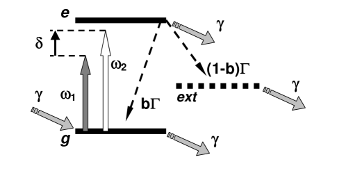
FIG. 1.: Level scheme considered for the model. The ground level $g$ and the excited level $e$ are degenerate with total angular momentum $F_{g}$ and $F_{e}$ respectively. Vertical arrows: excitation fields. Black dashed arrows: radiative decay. Oblique gray arrows: arrival and departure from the interaction zone.

Let consider a homogeneous ensemble of atoms at rest. However, in order to simulate the effect of a finite interaction time of the atoms with the light, we assume that the atoms escape the interaction region at a rate $\gamma$ , $(\gamma\ll\Gamma)$. This escape is compensated, at steady-state, by the arrival of fresh atoms in the ground state.

The atoms are submitted to the action of a magnetic field $B$ and two classical optical fields:

$$\vec{E}_{j}(t)=E_{j}\hat{e}_{j}e^{i\omega_{j}t}+E_{j}^{*}\hat{e}_{j}^{*}e^{-i\omega_{j}t},\ (j=1,2)$$ (1)

$\widehat{e}_{j}$ are complex polarization vectors. The Hamiltonian of the system can be written as:

$$H(t)=H_{0}+V_{1}\left(t\right)+V_{2}\left(t\right)$$ (2)

with:

$$H_{0} = H_{A}+H_{B}$$ (3)

$$H_{A} = \hbar\left(P_{e}\omega_{e}+P_{g}\omega_{g}\right)$$ (4)

$$H_{B} = (\beta_{g}P_{g}+\beta_{e}P_{e})F_{z}B$$ (5)

$$V_{j} = E_{j}\hat{e}_{j}\cdot\vec{D}_{ge}e^{i\omega_{j}t}+E_{j}^{*}\hat{e}_{j}^{*}\cdot\vec{D}_{eg}e^{-i\omega_{j}t}$$ (6)

here $P_{g}$ and $P_{e}$ are the projectors on the ground and excited manifolds respectively. $\beta_{g}$ and $\beta_{e}$ are the gyromagnetic factors of levels $g$ and $e$ respectively. $F_{z}$ is the component of the total angular momentum operator $\vec{F}$ along the magnetic field direction. $\vec{D}_{ge}=\vec{D}_{eg}^{\dagger}=P_{g}\vec{D}P_{e}$ is the lowering part of the atomic dipole operator (we assume that $P_{g}\vec{D}P_{g}=P_{e}\vec{D}P_{e}=0$). In Eq. 6 the usual rotating wave approximation is used.

The temporal evolution of the atomic density matrix $\rho$ is governed by the master equation [29]:

$$\frac{\partial\rho}{\partial t} = -\frac{i}{\hbar}\left[H,\rho\right]-\frac{\Gamma}{2}\left\{P_{e,}\rho\right\}$$ (8)

$$+b\Gamma\sum_{q=-1,0,1}Q_{ge}^{q}\rho Q_{eg}^{q}-\gamma\left(\rho-\rho_{0}\right)$$

where $Q_{ge}^{q}=Q_{eg}^{q\dagger}\ \left(q=-1,0.1\right)$ are the standard components of the dimensionless operator:

$$\vec{Q}_{ge}=\sqrt{2F_{e}+1}\frac{\vec{D}_{ge}}{\left\langle g\|\vec{D}\|e\right\rangle}$$ (9)

$F_{e(g)}$ is the total angular momentum of the excited(ground) state and $\left\langle g\|\vec{D}\|e\right\rangle$ is the reduced matrix element of the electric dipole operator.

The first term on the right hand side Eq. 8 represents the free atomic evolution in the presence of the two optical fields and the magnetic field. The remaining terms correspond to atomic relaxation. The second term on the right hand side accounts for the radiative relaxation of the excited state. The third term describes the feeding of the ground level by atoms decaying from the excited state. The last term phenomenologically accounts for the finite interaction time and ensures the relaxation of the system, in the absence of optical fields, to the thermal equilibrium state assumed to be described by the density matrix $\rho_{0}=P_{g}/(2F_{g}+1)$ corresponding to an isotropic distribution of the atomic population in the ground-state. Since there is no specific ground-state relaxation mechanism and $\gamma\ll\Gamma$, the rate $\gamma$ effectively plays the role of a ground-state relaxation coefficient.

In order to find the response of the system to the two fields we first consider the effect of field $E_{1}$ (hereafter designated as pump field) to all orders. Next, we calculate the effect of field $E_{2}$ (probe field) to first order. This procedure is analogous to the employed in the classical deduction of Mollow[3].

To obtain the response of the atomic system to the pump it is convenient to introduce the slowly varying matrix $\sigma_{0}$ given by:

$$\sigma^{0} = \sigma_{gg}^{0}+\sigma_{ee}^{0}+\sigma_{ge}^{0}+\sigma_{eg}^{0}$$ (10)

$$\sigma_{gg}^{0} = P_{g}\rho P_{g}$$ (11)

$$\sigma_{ee}^{0} = P_{e}\rho P_{e}$$ (12)

$$\sigma_{ge}^{0} = P_{g}\rho P_{e}e^{-i\omega_{1}t}$$ (13)

$$\sigma_{eg}^{0} = P_{e}\rho P_{g}e^{i\omega_{1}t}$$ (14)

after substitution into Eq. 8 (with $V_{2}=0$) one has for the steady state value of $\sigma^{0}$ the equation:

$$-\gamma\rho_{0} = -\frac{i}{\hbar}\left[H_{0}+\bar{V}_{1}-\hbar\omega_{1}P_{e},\sigma^{0}\right]-\frac{\Gamma}{2}\left\{P_{e},\sigma^{0}\right\}$$ (16)

$$+b\Gamma\sum_{q=-1,0,1}Q_{ge}^{q}\sigma^{0}Q_{eg}^{q}-\gamma\sigma^{0}$$

with:

$$\bar{V}_{1}=E_{1}\hat{e}_{1}\cdot\vec{D}_{ge}+E_{1}^{*}\hat{e}_{1}^{*}\cdot\vec{D}_{eg}$$ (17)

Eq. 16 represents a system of coupled linear equations involving the coefficients of the density matrix $\sigma^{0}$. We have numerically solved this system by employing a Liouville space formalism[30, 31] in which the state of the system is represented by a vector ${\bf x}$ whose elements are the coefficients of the density matrix $\sigma^{0}$. In the Liouville space Eq. 16 can be put into the form ${\cal L}{\bf x}={\bf x}_{{\bf 0}}$ (${\cal L}$ is a linear operator and ${\bf x}_{{\bf 0}}$ a constant vector) and readily inverted.

The relaxation term describing the return of the unperturbed system to equilibrium (fourth term in the right hand side of Eq. 16), as well as the possible escape to external levels when $b<1$, do not conserve the total population. In consequence, the solution of Eq. 16 must be normalized by the total number of atoms $N=n_{g}+n_{e}+n_{ext}$ where $n_{g}$, $n_{e}$ and $n_{ext}$ are the populations of the ground level, excited level and external level(s) respectively. Since at steady state the population of the external level(s) obeys the balance equation: $\Gamma(1-b)n_{e}=\gamma n_{ext}$ we have:

$$N=n_{g}+n_{e}[1+(1-b)\Gamma/\gamma]$$ (18)

where $n_{g}$ and $n_{e}$ are the ground and excited-state populations obtained from the numerical solution of 16 respectively. After normalization the solution of Eq. 16, $\sigma^{0}$ fully accounts for the preparation of the system by the pump. This includes effects such as optical saturation and induced coherence between ground and excited states, orientation and alignment due to Zeeman optical pumping and depopulation.

To analyze the effect to first order of the probe field on the atom + pump system, we seek a solution of Eq. 8 under the form[3]:

$$\rho_{gg}(t) = P_{g}\rho\left(t\right)P_{g}=\sigma_{gg}^{0}+\sigma_{gg}^{+}e^{i\delta t}+\sigma_{gg}^{-}e^{-i\delta t}$$ (19)

$$\rho_{ee}(t) = P_{e}\rho\left(t\right)P_{e}=\sigma_{ee}^{0}+\sigma_{ee}^{+}e^{i\delta t}+\sigma_{ee}^{-}e^{-i\delta t}$$ (20)

$$\rho_{ge}(t) = P_{g}\rho\left(t\right)P_{e}=e^{i\omega_{1}t}\left(\sigma_{ge}^{0}+\sigma_{ge}^{+}e^{i\delta t}+\sigma_{ge}^{-}e^{-i\delta t}\right)$$ (21)

$$\rho_{eg}(t) = P_{e}\rho\left(t\right)P_{g}=e^{-i\omega_{1}t}\left(\sigma_{eg}^{0}+\sigma_{eg}^{+}e^{i\delta t}+\sigma_{eg}^{-}e^{-i\delta t}\right)$$ (22)

with $\delta=\omega_{2}-\omega_{1}$. After substitution into Eq.8 and keeping only terms to first order in $E_{2}$ one has the following system of linear equations coupling $\sigma_{ge}^{+}$, $\sigma_{eg}^{+}$, $\sigma_{gg}^{+}$ and $\sigma_{ee}^{+}$:

$$iE_{2}\widehat{(e}_{2}.\vec{D}_{ge})\sigma_{eg}^{0} = -i\left[H_{g},\sigma_{gg}^{+}\right]-i\hbar\delta\sigma_{gg}^{+}+b\hbar\Gamma\sum_{q=-1,0,1}Q_{ge}^{q}\sigma_{ee}^{+}Q_{eg}^{q}$$ (24)

$$-\hbar\gamma\sigma_{gg}^{+}-i\left(E_{1}\hat{e}_{1}\cdot\vec{D}_{ge}\sigma_{eg}^{+}-\sigma_{ge}^{+}E_{1}^{*}\hat{e}_{1}^{*}\cdot\vec{D}_{eg}\right)$$

$$-iE_{2}\sigma_{eg}^{0}\widehat{(e}_{2}.\vec{D}_{ge}) = -i\left[H_{e},\sigma_{ee}^{+}\right]-i\hbar\delta\sigma_{ee}^{+}-\hbar\left(\Gamma+\gamma\right)\sigma_{ee}^{+}$$ (26)

$$-i\left(E_{1}^{*}\hat{e}_{1}^{*}\cdot\vec{D}_{eg}\sigma_{ge}^{+}-\sigma_{eg}^{+}E_{1}\hat{e}_{1}\cdot\vec{D}_{ge}\right)$$

$$i\left(E_{2}\widehat{e}_{2}.\vec{D}_{ge}\sigma_{ee}^{0}-\sigma_{gg}^{0}E_{2}\widehat{e}_{2}.\vec{D}_{ge}\right) = -i\left(H_{g}\sigma_{ge}^{+}-\sigma_{ge}^{+}H_{e}\right)-i\hbar\left(\delta+\omega_{1}\right)\sigma_{ge}^{+}-\hbar\left(\frac{\Gamma}{2}+\gamma\right)\sigma_{ge}^{+}$$ (28)

$$-i\left(E_{1}\hat{e}_{1}\cdot\vec{D}_{ge}\sigma_{ee}^{+}-\sigma_{gg}^{+}E_{1}\hat{e}_{1}\cdot\vec{D}_{ge}\right)$$

$$0 = -i\left(H_{e}\sigma_{eg}^{+}-\sigma_{eg}^{+}H_{g}\right)-i\hbar\left(\delta-\omega_{1}\right)\sigma_{eg}^{+}-\hbar\left(\frac{\Gamma}{2}+\gamma\right)\sigma_{eg}^{+}$$ (30)

$$-i\left(E_{1}^{*}\hat{e}_{1}^{*}\cdot\vec{D}_{eg}\sigma_{gg}^{+}-\sigma_{ee}^{+}E_{1}^{*}\hat{e}_{1}^{*}\cdot\vec{D}_{eg}\right)$$

It is convenient at this point to introduce the non-Hermitian matrix $\sigma$ defined as:

$$\sigma=\left(\begin{array}[]{ll}\sigma_{gg}^{+}&\sigma_{ge}^{+}\\ \sigma_{eg}^{+}&\sigma_{ee}^{+}\end{array}\right)$$ (31)

After inspection it can be seen that Eqs.26 can be then rewritten in the operatorial form:

$$i\left[\frac{\Omega_{2}}{2},\sigma_{0}\right] = -\frac{i}{\hbar}\left[H_{0}+\bar{V}_{1}-\hbar\omega_{1}P_{e},\sigma\right]$$ (34)

$$-i\delta\sigma-\frac{\Gamma}{2}\left\{P_{e},\sigma\right\}-\gamma\sigma$$

$$+b\Gamma\sum_{q=-1,0,1}Q_{ge}^{q}\sigma Q_{eg}^{q}$$

where we have introduced the probe Rabi frequency $\Omega_{2}=(2\vec{E}_{2}\cdot\vec{D}_{ge})/\hbar.$

Eq. 34 is numerically solved by the same Liouville-space procedure used to solve Eq. 16. The resulting value of the operator $\sigma$ simultaneously provides the values of the four matrices $\sigma_{ge}^{+}$, $\sigma_{eg}^{+}$, $\sigma_{gg}^{+}$ and $\sigma_{ee}^{+}$ each of which contains useful information on the atomic response as will be now discussed.

The information concerning the optical atomic polarization oscillating at the probe frequency is contained in matrix $\sigma_{ge}^{+}$ (see Eqs. 21). The complex macroscopic atomic polarization at the frequency of the probe is given by:

$$\vec{P}\left(\omega_{2}\right)=\varepsilon_{0}\chi\vec{E}_{2}=nTr\left(\sigma_{ge}^{+}\vec{D}_{eg}\right)$$ (35)

where $\varepsilon_{0}$ is the vacuum dielectric constant, $\chi=\chi^{\prime}+i\chi^{\prime\prime}$ is the complex susceptibility tensor and $n$ is the atom density. From the complex polarization we get the probe absorption coefficient as:

$$\alpha\left(\omega_{2}\right)=k_{2}(\widehat{e}_{2}\cdot\chi^{\prime\prime}\widehat{e}_{2})=\frac{nk_{2}}{E_{2}}\widehat{e}_{2}\cdot Imag\left[Tr\left(\sigma_{ge}^{+}\vec{D}_{eg}\right)\right]$$ (36)

$k_{2}$ is the modulus of the probe wave-vector.

Similarly, the dielectric tensor $\varepsilon=\varepsilon_{0}(1+\chi^{\prime})$ describing the dispersion of the probe by the atomic medium obeys:

$$\widehat{e}\cdot\varepsilon\ \widehat{e}_{2}=\varepsilon_{0}\left\{1+\frac{n}{E_{2}}\widehat{e}\cdot Real\left[Tr\left(\sigma_{ge}^{+}\vec{D}_{eg}\right)\right]\right\}$$ (37)

where $\widehat{e}$ is an arbitrary unit vector.

The matrix $\sigma_{eg}^{+}$ contains information about the off-diagonal elements of the density matrix evolving at the frequency $2\omega_{1}-\omega_{2}$. The corresponding atomic polarization is responsible for the generation of a new optical field at this frequency by four wave-mixing (FWM) [32].

The intensity of the field generated by FWM satisfies:

$$I_{FWM}(2\omega_{1}-\omega_{2})\varpropto n^{2}\left|Tr\left(\sigma_{eg}^{+}\vec{D}_{ge}\right)\right|^{2}$$ (38)

The matrices $\sigma_{gg}^{+}$ and $\sigma_{ee}^{+}$ contain information concerning the pulsation of the ground and excited state populations at the difference frequency $\delta$ between the pump and the probe fields. Opposite fluctuation of the total population occurs in the ground and the excited state. The effect of the modulation of the population of the excited state can be directly observed as an oscillating component (at frequency $\delta$) of the fluorescence emitted by the atoms. The pulsation of the total fluorescence power emitted per atom is:

$$\Delta W(t)=2b\Gamma\hbar\omega_{0}\left[Tr\left(\sigma_{ee}^{+}\right)e^{i\delta t}+cc\right]$$ (39)

Finally, the matrices $\sigma_{gg}^{+}$ and $\sigma_{ee}^{+}$ also provide information about population redistribution and coherence among Zeeman sublevels (orientation and/or alignment) in the ground or excited state due to the simultaneous interaction with the pump and probe fields. This result in additional observables evolving at frequency $\delta$ . As an example, the oscillating magnetic dipole induced in the ground state by the coherent interaction with the pump and probe fields is given by:

$$\vec{M}_{g}(t)=n\beta_{g}\left[Tr\left(\sigma_{gg}^{+}\vec{F}\right)e^{i\delta t}+cc\right]$$ (40)

In the following sections we present and discuss the spectroscopic features of the atomic response. Particular attention is given to the absorption and population pulsation spectra for which experimental results are presented.

B Probe absorption spectra.

1 Spectra with zero magnetic field.

We initially consider the results obtained for motionless atoms in the absence of a magnetic field. Some examples of level configurations and the corresponding probe absorption spectra for particular choices of the polarizations of the pump and probe fields are shown in Figs. 2 and 3. In general, the spectra are composed of a Lorentzian peak, whose width is given by the excited state relaxation rate and in most cases, a narrow resonance (hereafter named coherence resonance) arising when the frequency offset $\delta\$between pump and probe satisfies the condition for two-photon Raman resonances between Zeeman sublevels. In the particular case of Figs. 2 and 3 a unique coherence resonance at $\delta=0$ occurs since $B=0$. Let us first discuss the case of closed (cycling) transitions. Depending on the choice of the total angular momentum of the ground and excited states the coherence resonance corresponds to a reduction in the absorption (EIT) or an enhancement of the absorption (EIA)[27, 28]. No coherence resonance appears for some configurations. As discussed in Ref. [28] EIA occurs provided that three conditions are satisfied: $i)$ The transition is closed, $ii)\ F_{g}>0$ and $iii)$ $F_{g}<F_{e}$. This is the case of Fig. 2 (a). On the other hand, EIT occurs if $F_{g}\geq F_{e}$ and $F_{g}>0$ [Fig. 2 (b)][33]. Finally, no coherence resonance occurs if $F_{g}=0$ [Fig. 2(c)].

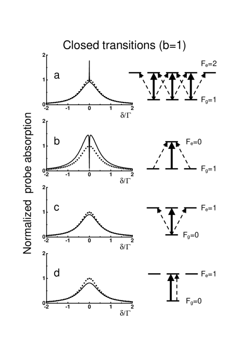
FIG. 2.: Probe absorption spectra as a function of the frequency offset $\delta$ (solid lines) with $B=0$ and $\Omega_{1}/\Gamma\equiv 2E_{1}\left\langle g\left\|D\right\|e\right\rangle/\left(\hbar\Gamma\right)=0.4,\ \gamma/\Gamma=0.001$ for different closed ($b=1$) atomic transitions. The spectra are normalized to the maximum of the linear absorption (represented in dotted lines). The pump and probe polarizations are linear and orthogonal in $a$, $b$, $c$ and parallel in $d$. The corresponding angular momenta and magnetic sublevels scheme is shown in each case. Solid (dashed) arrows represent the pump (probe) field.

When the transition is open $\left(b<1\right)$, the previous results are modified. In addition to an overall reduction of the absorption as a consequence of population loss to the external levels significant changes concern the coherence resonance. When $F_{g}<F_{e}$ and $Fg>0$ for sufficiently large values of the escape rate $(1-b)\Gamma$ compared to $\gamma$ a narrow transparency dip appears at the place of the absorption enhancement observed for cycling transitions[5] [Fig. 3 (a)]. A similar absorption dip is present in the case of the $F_{g}=0\rightarrow F_{e}=1$ transition with equal pump and probe polarizations [Fig. 3 (d)]. A situation that corresponds to the pure two-level system. The origin of the narrow dip is the same in the two cases. It can be attributed to the resonant scattering of the probe field by the modulation in the atomic populations induced by the two fields[1, 32]. As in the case of closed transitions, no narrow resonance occurs for the $F_{g}=0\rightarrow F_{e}=1$ transition when the polarizations are orthogonal ($V$ system) [Fig. 3 (c)]. Finally when $F_{g}\geq F_{e}$ [Fig. 3 (b)] a large EIT resonance is observed. As in the case of cycling transitions, the transparency dip is essentially associated to the falling of the system into a dark state in the ground level rather than to an increased escape to external levels[18].

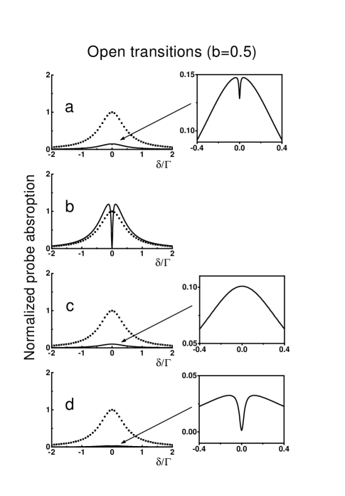
FIG. 3.: Probe absorption spectra as a function of the frequency offset $\delta$ (solid lines) with $B=0$ and $\Omega_{1}/\Gamma\equiv 2E_{1}\left\langle g\left\|D\right\|e\right\rangle/\left(\hbar\Gamma\right)=0.4,\ \gamma/\Gamma=0.001$ for different open ($b=0.5$) atomic transitions. The spectra are normalized to the maximum of the linear absorption (represented in dotted lines). The fields polarizations are the same as in the corresponding case of Fig. 2. The insets represent enlarged views around the center of the spectra.

In the present context, both EIT and EIA appear in the same theoretical framework as the result of the coherent interaction of the degenerate atomic system with the two fields. This result clearly stresses the role of the atomic dynamics at the common origin of the two phenomena. It is nevertheless interesting to point out that from a different point of view, EIT has been usually associated to the existence of a stationary dark-state (a quantum superposition of ground state sublevels not coupled to the excited state) in which the atomic population is trapped [19]. This arises the question of whether a corresponding “bright-state” can be identified to correspond to EIA.

The identification of the steady state of the system, in the case of EIA, as well as for EIT, is greatly simplified in the present context (degenerate levels, $B=0$) since at resonance ($\delta=0$) the pump and probe fields reduce to a single field. Consequently, the stationary state of the system is simply the result of the optical pumping of the degenerate two level-system by the unique field. When the conditions for EIT are satisfied ($F_{g}\geq F_{e}$) this results in the falling of the system into the uncoupled sub-space of the ground level. When EIA occurs ($F_{g}<F_{e}$), all the ground level manifold is affected by the light. In this case, the steady state of the system is shared by the ground and the excited level. Unlike in the case of EIT, the steady state corresponding to an EIA resonance is obviously not stable (in the absence of the fields) since it is affected by spontaneous emission.

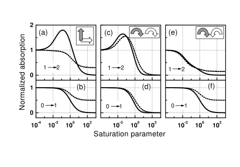
FIG. 4.: Absorption at $\delta=0$, $B=0,\ \gamma/\Gamma=0.001$ for different closed atomic transitions and different pump and probe polarizations as a function of the saturation parameter $S$ $\equiv 2[2E_{1}\left\langle g\left\|D\right\|e\right\rangle/\left(\hbar\Gamma\right)]^{2}$ (solid lines). The absorption is normalized to the maximum linear absorption. The dashed lines represent the incoherent optical pumping contribution (see text). The corresponding $F_{g}\rightarrow F_{e}=F_{g}+1$ transition is indicated in each case. The pump and probe polarizations are linear and orthogonal ($a,b$), circular and equal ($c,d$) and circular and opposite ($e,f$).

We address now the question of the amplitude of the coherence resonance in the probe absorption. We restrict ourselves to closed transitions of the type $F_{g}\rightarrow F_{e}=F_{g}+1$ where EIA occurs. The coherence resonance amplitude depends on the angular momenta of the levels considered, the optical polarizations, the pump intensity and the rate $\gamma$. Some examples of the intensity dependence of the absorption at $\delta=0$ for different $F_{g}$ ($F_{e}=F_{g}+1$) and the optical polarizations are shown in Fig. 4. The absorption is normalized to the probe absorption in the absence of the pump and it is presented as a function of the saturation parameter $S\equiv 2[2E_{1}\left\langle e\left\|D\right\|g\right\rangle/(\hbar\Gamma)]^{2}$ which is proportional to pump intensity. Also shown in Fig. 4 is the contribution to the probe absorption which is only due to the incoherent optical pumping by the pump field. This contribution, obtained taking $\bar{V}_{1}=0$ in Eq. 34, includes the effect of Zeeman optical pumping and optical saturation produced by the pump field but ignores coherent two-photon processes involving both fields. The maximum resonant enhancement of the absorption occurs for linear and perpendicular pump and probe polarizations. Notice that in this case, the incoherent optical pumping contribution remains below the linear absorption for all intensities. When the polarization of the two fields are the same, (Fig. 4c,d) the coherent enhancement of the absorption is smaller and there is a significant contribution to the absorption enhancement from incoherent optical pumping. No absorption enhancement occurs for circular and opposite pump and probe polarizations Fig. 4(e,f). Notice that Figs. 4(d) and 4(f) correspond to the pure two-level and V schemes respectively.

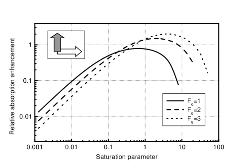
FIG. 5.: Relative absorption enhancement $\eta=(\alpha-\alpha_{L})/\alpha_{L}\$at $\delta=0$, $B=0,\ \gamma/\Gamma=0.001$ for different $F_{g}\rightarrow F_{e}=F_{g}+1$ closed atomic transitions as a function of the saturation parameter $S$ ($\alpha_{L}$ is the maximum linear absorption). The pump and probe polarizations are linear and orthogonal.

As is also the case for EIT[34], in the weak pump limit the amplitude of the EIA resonance is linear in the pump intensity as shown in Fig. 5 for linear and perpendicular pump and probe polarizations [35]. Notice that for a weak pump field the higher absorption enhancement factor is obtained for $F_{g}=1$ and decreases for increasing $F_{g}$. However, the maximum value of the enhancement increases with $F_{g}$ for the values considered in Fig. 5. The maximum absorption enhancement is obtained for a saturation parameter close to unity. At higher intensities the absorption at zero frequency offset decreases as a consequence of the dynamic Stark effect[3].

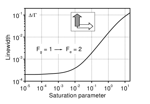
FIG. 6.: Linewidth $\Delta$ (half width at half maximum) of the coherence absorption resonance at $\delta=0$, $B=0,\ \gamma/\Gamma=10^{-4}$ for the closed $F_{g}=1\rightarrow F_{e}=2$ transition as a function of the saturated parameter $S$. The pump and probe polarizations are linear and orthogonal.

The linewidth $\Delta$ of the EIA and EIT resonances (FWHM) is determined, at low pump field intensities, by the finite interaction time. It is given by $\Delta=2\gamma$. At larger pump intensities power broadening occurs with $\Delta$ increasing linearly with the pump intensity (see Fig. 6)[27]. This behavior is analogous to the observed for EIT resonances in $\Lambda$ configurations [19].

The sharp variations in the absorption corresponding to EIT or EIA resonances are accompanied by modifications of the refractive index. Fig. 7 shows the calculated refractive index variation for the probe field for two different closed transitions with linear and orthogonal pump and probe polarizations. Very steep normal and anomalous dispersion takes place for EIT and EIA respectively[36] corresponding to small absolute values of the group velocity which may be negative in the case of EIA[37].

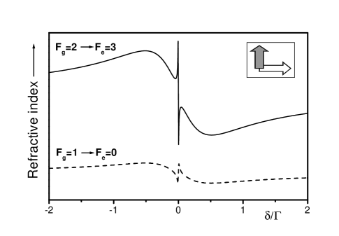
FIG. 7.: Refractive index spectra for the probe field as a function of the frequency offset $\delta$ for two closed atomic transitions. $B=0$, $\Omega_{1}/\Gamma=0.4,\ \gamma/\Gamma=0.001$. The pump and probe polarizations are linear and orthogonal. The vertical positions of the traces are arbitrary. The vertical scale is the same for both curves.

2 Spectra in the presence of a magnetic field.

The presence of a magnetic field removes the degeneracy of the atomic level. As a consequence, the narrow resonances corresponding to EIT or EIA split into several components. The position of each component is given by a resonance condition for a Raman transition between two ground-state Zeeman sublevels involving one pump photon and one probe photon. The selection rules determining the number of resonances are the same for EIT or EIA. However the spectra obtained under the same polarizations and intensities of the pump and probe fields, present some qualitative and quantitative differences in addition to the sign inversion. Fig. 8 present the comparison of the EIT and EIA spectra calculated for the closed transitions $F_{g}=3\rightarrow F_{e}=4$ and $F_{g}=2\rightarrow F_{e}=1$. It is interesting to point out that whenever it is allowed by the Raman selection rules, the line corresponding to transitions from Zeeman sublevels to themselves is present in the spectra. This is the case of Fig. 8a. The corresponding peak occurs at zero pump-probe frequency offset independently of the value of the magnetic field. Also for some combinations of the pump and probe polarizations (for instance $\sigma^{+}$ and $\sigma^{-}$ respectively) there is a unique resonance whose position depends on the value of the magnetic field (Fig. 8c).

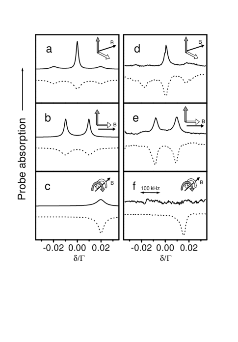
FIG. 8.: a-c: Calculated probe absorption spectra under the presence of a magnetic field ($\beta_{g}B/\Gamma=0.01,\ \Omega_{1}/\Gamma=0.3,\ \gamma/\Gamma=0.001$) for the transitions $F_{g}=3\rightarrow F_{e}=4$ (solid) and $F_{g}=2\rightarrow F_{e}=1$ (dashed). The vertical positions of the traces are arbitrary. The vertical scale is the same for all curves. d-f: Measured probe absorption spectra with the laser tuned to the transitions $5S_{1/2}(F_{g}=3)$ $\rightarrow 5P_{3/2}$(solid) and $5S_{1/2}(F_{g}=2)\rightarrow 5P_{3/2}$ (dashed) of ⁸⁵Rb under the presence of a magnetic field ($\beta_{g}B/2\pi\approx 50\ kHz,\ \Gamma/2\pi=5.9\ MHz$). The vertical positions of the traces are arbitrary. The vertical scale is the same for all curves.

C Four-wave-mixing spectra.

The importance of level degeneracy on FWM generation was long ago appreciated. It plays an essential role in connection with the study of collision-induced resonances[39, 7, 8]. Recently, FWM in a degenerate two-level system was used for the construction of a phase conjugate resonator[40]. We analyze now the predictions of our model concerning the generation of a new field by FWM according to Eq. 38.

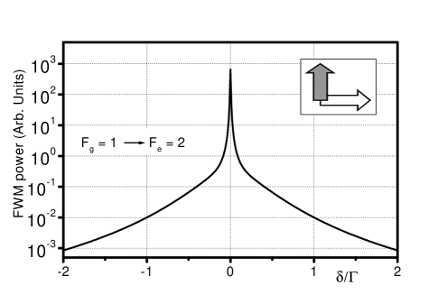
FIG. 9.: Power of FWM emission as a function of the frequency offset $\delta$ for the closed $F_{g}=1\rightarrow F_{e}=2$ transition ($B=0,\ \gamma/\Gamma=0.001)$. The pump and probe polarizations are linear and orthogonal.

When the conditions for coherence resonances are satisfied a large increase in the intensity of the field generated at frequency $2\omega_{1}-\omega_{2}$ occurs. The generated FWM power as a function of $\delta$ is presented in Fig. 9 in the case of orthogonal and linear pump and probe polarizations and no magnetic field (notice the vertical logarithmic scale). As seen the coherence resonance peak of FWM can be several orders of magnitude larger than the non-resonant background of width $\sim\Gamma$. The high contrast is a consequence of the triple resonant interaction of the three fields involved in the nonlinear mixing process [32].

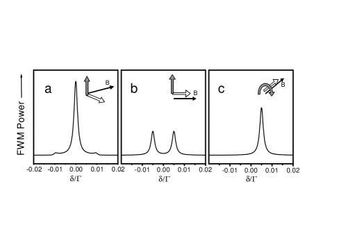
FIG. 10.: Power of FWM emission as a function of the frequency offset $\delta$ for the closed $F_{g}=1\rightarrow F_{e}=2$ transition under the presence of a magnetic field ($\beta_{g}B/\Gamma=0.005,\ \gamma/\Gamma=0.001$). The pump and probe polarizations are: $a)$ linear, orthogonal and transverse respect to $\vec{B}$. $b)$ linear, orthogonal and probe along $\vec{B}$. $c)$ pump circular transverse, probe linear along $\vec{B}$.

Under the presence of a magnetic field the FWM spectra splits into several peaks. Fig. 10 shows some examples of calculated spectra obtained for different pump and probe polarizations. The selection rules governing resonant FWM result from two simultaneous requirements on the pump and probe polarizations: $a)$ A three-photon transition from the ground to the excited level involving the absorption of two pump photons and the emission of one probe photon should be permitted. $b)$ An electric dipole transition should be allowed between the initial (ground) and the final (excited) sublevels connected by the three-photon processes. These rules are different from the rules corresponding to probe absorption. For instance, no coherence resonance in FWM occurs if the pump and probe polarizations are circular and opposite. However, absorption resonances are generally observable in this case.

To our knowledge, the results presented here constitutes the first detailed calculation of coherence resonances spectra in FWM involving Zeeman sublevels in degenerate two-level system.

D Population modulation spectra.

The modulation of the excited state population results in modulation of the emitted fluorescence according to Eq.39. This modulation has a similar origin than that discussed in the context of CPT in a driven $\Lambda$ system [41]. As mentioned in [41] the modulation in the fluorescence is intimately connected to FWM. In the context of the present paper, this connection is the natural consequence of the coupling between $\sigma_{ge}^{+}$, $\sigma_{eg}^{+}$, $\sigma_{gg}^{+}$ and $\sigma_{ee}^{+}$ described by Eq.34.

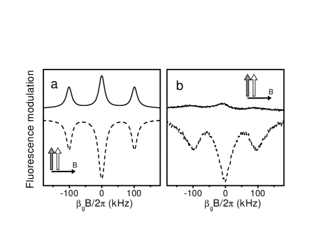
FIG. 11.: Fluorescence modulation at the frequency of the pump to probe offset $\delta/2\pi=200\ kHz$ as a function of magnetic field. $a)$ Calculated signal for the closed transitions $F_{g}=3\rightarrow F_{e}=4$ (solid) and $F_{g}=2\rightarrow F_{e}=1$ (dashed) with $\Omega_{1}/\Gamma=0.3,\ \gamma/\Gamma=0.001,\ \Gamma/2\pi=5.9\ MHz$). $b)$ Measured signal with the laser tuned to the transitions $5S_{1/2}(F_{g}=3)$ $\rightarrow 5P_{3/2}$(solid) and $5S_{1/2}(F_{g}=2)\rightarrow 5P_{3/2}$ (dashed) of ⁸⁵Rb. The pump and probe polarizations are linear, parallel and transverse with respect to $\vec{B}$. The vertical positions of the traces are arbitrary.

Population modulation is due to the coupling of the optical coherence induced by one of the fields between two Zeeman sublevels in the ground and the excited state with the second field. In consequence, it occurs when the two fields couple the same pair of excited and ground Zeeman sublevels. If the polarizations of the two fields are the same and correspond to a proper polarization with respect to the magnetic field orientation ($\sigma^{+}$, $\sigma^{-}$ or $\pi$), the modulated fluorescence present no resonance narrower than $\Gamma$ as a function of the pump to probe frequency offset. However, interesting interference effects, resulting in coherence resonances (linewidth determined by $\gamma$), occur for other pump and probe polarizations. Fig. 11(a,b) shows the calculated modulated component of the total fluorescence for two different transitions as a function of the magnetic field for fixed pump-probe frequency offset and the same transverse linear polarization. Three coherence resonances are present in this case. The central one corresponds to zero magnetic field. The positions of the two lateral peaks correspond to the conditions for resonant Raman transitions between Zeeman sublevels. The signs of the resonances are opposite in the case of transitions corresponding to EIA (Fig.11a) or EIT (Fig.11b). Notice the larger relative variation of the pulsation amplitude in the case of EIT.

E Oscillating magnetic dipole spectra.

The simultaneous interaction of an atomic system with two fields can result in the driving of Zeeman coherence in the ground state. This coherence can in turn be responsible for electromagnetic emission [42]. To illustrate this phenomenon, in the case of degenerate two-level system, we analyze the predictions of our model concerning the induced ground-state magnetic dipole oscillating at frequency $\delta$ (Eq.40).

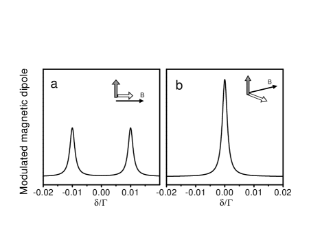
FIG. 12.: Calculated modulus of the ground state magnetic dipole modulated at frequency $\delta$ for $\beta_{g}B/\Gamma=0.01,\ \Omega_{1}/\Gamma=0.01,\ \gamma/\Gamma=0.001$. The pump and probe polarizations are: $a)$ pump linear transverse, probe linear along $\vec{B}$. $b)$ pump and probe linear orthogonal and transverse respect to $\vec{B}$.

The selection rules governing the oscillating magnetic dipole spectra differ from those of the previously analyzed processes. Some examples of the predicted oscillating magnetic dipole as a function of the magnetic field for fixed pump to probe frequency offset are shown in Fig.12. Coherence resonances in the oscillating dipole modulus take place when the two fields couple adjacent ground state Zeeman sublevels. This is the case of Fig.12$a$ corresponding to $\pi$ polarized pump and a transverse and linearly polarized probe. The coherence resonance illustrated in Fig.12$b$ corresponding to transverse, orthogonal linearly polarized pump and probe is somehow different since its position ($B=0$) does not correspond to a two photon process between different Zeeman sublevels. The resonance can be understood, in this case, as the result of interference between two non resonant two-photon processes. In every case the resonance width are determined by the relaxation rate $\gamma$.

III Experiments.

A Setup.

The experiments were performed on the D₂ line of ⁸⁵Rb. The experimental setup is similar to the one previously presented[27, 28]. We remind here the principal features. The pump and probe fields were generated from the output of a unique extended cavity diode laser. This laser was locked, with the help of an external servo loop, to a saturated absorption line obtained from a reference Rb vapor cell. The frequency uncertainty of the locked laser is less than 1 MHz over several minutes. Most of the power of the laser beam was used as the pump field. The probe field was generated by frequency shifting a fraction of the laser beam with two consecutive acousto-optic modulators, one of them driven by a variable RF source. In this way two mutually coherent pump and probe waves were generated with tunable frequency offset $\delta$. The polarization of the two fields were independently controlled. Perfect overlap between the two fields was achieved by propagating them along a 50 cm single mode optical fiber that did not significantly modify the polarizations. The light was sent through a 2 cm long vapor cell. The power of the pump and probe at the atomic sample were $0.8\ mW$ and $50\ \mu W$ respectively. The atomic cell was placed within Helmholtz coils for magnetic field control. For the probe absorption measurements, the pump beam was blocked by a polarizer, (extinction ratio larger than 200) while the probe intensity was detected with a photodiode. To enhance sensitivity and signal to noise ratio, a two-frequency lock-in detection technique was used [43]. For this, the pump and probe fields were chopped at the frequencies $f_{1}$ and $f_{2}$ (around 1 kHz) respectively and the photodiode output current was analyzed at frequency $f_{1}+f_{2}$ by a lock-in amplifier. By this means only the non-linear component of the probe transmission, dependent on the pump and probe intensities, was detected.

For the measurement of the excited state population modulation, the atomic fluorescence was collected with a large area photodiode (1cm diameter) situated close to the vapor cell. The photodiode current was sent to an RF frequency analyzer operating in the zero span mode, that is measuring the RF input amplitude at a fixed frequency set equal to the probe to pump frequency offset $\delta$. A fixed value of $\delta=200\ kHz$ was used while the longitudinal magnetic field at the cell was scanned over a few hundred milligauss around the zero magnetic field. During these measurements the cell was surrounded by a $\mu-$metal shield reducing the ambient magnetic field to less than $10\ mG$. The scanning of the longitudinal magnetic field was accomplished with coils placed inside the magnetic shield.

B Results.

1 Probe absorption.

Fig. 8(d-f) shows several examples of probe absorption spectra obtained for different orientations of the magnetic field and the optical fields polarizations. In each figure division, two spectra obtained from the excitation of the lower and the upper ground-state hyperfine levels of ⁸⁵Rb under the same optical fields intensities and polarizations are presented. When the lower ground-state hyperfine level is addressed EIT resonances are observed while in the case of the upper ground-state hyperfine level EIA occurs. The agreement between the predictions of the model and the observations is quite satisfactory. This agreement may seem rather surprising since in the vapor cell, due to the velocity distribution, three different atomic transitions, one closed and two open contribute to the signal in each case. On all open transitions as well as on the closed $F_{g}=2\rightarrow F_{e}=1$ transition EIT occurs. Only on the $F_{g}=3\rightarrow F_{e}=4$ transition EIA takes place [28]. However, due to optical pumping the absorption signal is essentially determined by the closed transitions resulting in the qualitative agreement with the theoretical prediction. Some differences are nevertheless observed: The relative strength of the EIA and EIT transitions are not the same than in the calculation and the small EIA resonance predicted in Fig.8c is not visible in the experiment (Fig.8f). We have verified that a closer agreement between the experimental observation and theory can be achieved by taking into account the excited state hyperfine structure and the atomic velocity distribution according to the procedure described in [28].

2 Modulated fluorescence.

The measured signal corresponding to the fluorescence modulated at frequency $\delta=200kHz$ is presented in Fig.11(c,d). The traces are composed of a constant background over which narrow resonances are visible. The modulated fluorescence is of the order of 10^-3 times the total fluorescence. The contrast of the coherence resonances with respect to the constant background is larger in the case of the lower ground state hyperfine level ($\sim 20\%$) compared to that of the upper ground state hyperfine level ($\sim 5\%$). The width of the peaks are determined by magnetic field inhomogeneities.

The main features in the observed curves are in good qualitative agreement with the predictions based on the theoretical model valid for atoms at rest. This indicates that, as in the case of absorption, the spectra are dominated by the corresponding cycling transition and that the influence of the Doppler effect on the coherence resonances positions is not essential. More elaborate calculations including velocity integration and summation over excited state hyperfine levels provide closer agreement with the observations [44]. The results reported here constitute, to our knowledge, the first demonstration of the observation of coherence resonances through the analysis of fluorescence modulation.

C Conclusions.

The response of a degenerate two-level atomic system to the simultaneous presence of a pump and a probe field has been examined with the help of a theoretical model allowing the numerical calculation of the atomic response in a large variety of situations. Based on this model, the manifestations of the coherent nature of the atom-field interaction on different observables were analyzed and the corresponding spectra calculated. Most of these observables present narrow coherence resonances whose width is essentially determined by the ground-state relaxation. The dependence of the coherence resonances spectra on the atomic transition, the optical fields polarizations and magnetic field was investigated. Two experimental observations are compared with the predictions of the model: the probe absorption spectra in the presence of a magnetic field and the modulated fluorescence dependence on magnetic field.

The results reported in this paper illustrate the richness of the coherent response of degenerate two level systems. Further study of coherence resonances in degenerate two-level systems should broaden our present understanding of coherent processes. In addition, it may provide the base for interesting applications such as magnetic field measurement[22] or refractive index manipulation[37].

D Acknowledgments.

The author wish to thank D. Bloch and M. Ducloy for stimulating discussions. This work was supported by CONICYT, CSIC and PEDECIBA (Uruguayan agencies) and ECOS (France).

REFERENCES

- [1] E.V.Baklanov and V.P.Chebotaev, Zh.Eksp.Teor.Fiz. 61, 922 (1971) [Sov. Phys. JETP 34, 490 (1972)].
- [2] S. Haroche, F. Hartmann, Phys. Rev. A. 6, 1280 (1972).
- [3] B.R. Mollow, Phys. Rev. A 3, 2217 (1972).
- [4] V.S. Lethokhov and V.P. Chebotayev, Nonlinear Laser Spectroscopy, Springer Series in Optical Sciences Vol. 4, Springer-Verlag, Berlin (1977).
- [5] A. Wilson-Gordon and H. Friedmann, Optics Lett. 14, 390 (1989).
- [6] W. Happer, Reviews of Modern Physics, 44, 169 (1972) and references therein.
- [7] P.R. Berman, D.G. Steel, G. Khitrova and J. Liu, Phys. Rev. A 38, 252 (1988).
- [8] P.R. Berman, Phys. Rev. A 43, 1470 (1991).
- [9] J.Guo and P.R. Berman, Phys. Rev. A 47, 4128 (1993).
- [10] Bo Gao, Phys. Rev. A 48, 2443 (1993).
- [11] Bo Gao, Phys. Rev. A 49, 3391 (1994).
- [12] C. Cohen-Tannoudji and S. Reynaud, J. Physique 38, L-173 (1977).
- [13] Bo Gao, Phys. Rev. A 50, 4139 (1994).
- [14] J.R. Morris and B.W. Shore, Phys. Rev. A 27, 906 (1983).
- [15] S.I. Kanorsky, A. Weis, J. Wurster and T.W. Hänsch, Phys. Rev. A 47, 1220 (1993).
- [16] V. Milner, B.M. Chernobrod and Y. Prior, Europhys. Lett. 34, 557 (1996).
- [17] A.V. Taichenachev, A.M. Tumaikin and V.I. Yudin. SPIE Vol. 3485, 202 (1998).
- [18] V. Milner and Y. Prior, Phys. Rev. Lett. 80, 940 (1998).
- [19] E.Arimondo, Coherent population trapping, Progress in Optics XXXV, 257 (1996) and references therein.
- [20] see S. E. Harris, Physics Today, 50(7) 36 (1997) and references therein.
- [21] J. Lawall et al, Phys. Rev. Lett. 75, 4194 (1995).
- [22] M.O. Scully and M. Fleischhauer, Phys. Rev. Lett. 69, 1360 (1992). H. Lee, M. Fleischhauer and M. Scully, Phys. Rev. A 58, 2587 (1998) and references therein.
- [23] M.O. Scully, Phys, Rev. Lett. 67, 1855 (1991). A.S. Zibrov et al, Phys. Rev. Lett. 76, 3935 (1996).
- [24] S.E. Harris, J.E. Field and A. Imamoglu, Phys. Rev. Lett. 64, 1107 (1990).
- [25] S.E. Harris, J.E. Field and A. Kasapi, Phys. Rev. A 46, R29 (1992).
- [26] L.V. Hau, S.E. Harris, Z. Dutton, and C.H. Behroozi, Nature 397, 594 (1999). M.M. Kash, V.A.Sautenkov, A.S. Zibrov, L. Hollberg, G.H. Welch, M.D. Lukin, Yu. Rostovtsev, E.S. Fry, and M. Scully, Phys. Rev. Lett. 82, 5229 (1999).
- [27] A.M. Akulshin, S. Barreiro and A. Lezama, Phys. Rev. A 57, 2996 (1998).
- [28] A. Lezama, S. Barreiro and A.M. Akulshin, Phys. Rev. A. to be published (1999).
- [29] C. Cohen-Tannoudji in Frontiers of Laser Spectroscopy, Vol. 1. Ed. R. Balian, S. Haroche and S. Liberman. North Holland, Amsterdam (1977).
- [30] C. Feuillade and P.R. Berman, Phys, Rev. A 29, 1236 (1984) and references therein.
- [31] N. Cyr, PhD. Thesis, Laval University, (1990).
- [32] Y.R. Shen, The principles of nonlinear optics, J. Wiley & Sons, New York (1984).
- [33] V.S. Smirnov, A.M. Tumakin and V.I. Yudin, Zh. Eksp. Teor. Fiz. 96, 1613 (1989) [Sov. Phys. JETP 89, 913 (1989)].
- [34] See for instance M.O. Scully and M.S. Zubairy, Quantum Electronics, Cambridge University Press, Cambridge (1997).
- [35] A.V. Taichenachev, A.M.Tumaikin, and V.I. Yudin, Lett. JETP 69, (1999) [Pis’ma ZhETF 69, 776 (1999)].
- [36] O. Shmiddt, R. Wynands, Z. Hussein and D. Meschede, Phys. Rev. A 53, R27 (1996).
- [37] A. Akulshin, S. Barreiro and A. Lezama, Submitted to Phys. Rev. Lett. (1999).
- [38] M.P. Gorza, B. Decomps, M. Ducloy, Optics Commun. 8, 323 (1973).
- [39] L.J. Rothberg and N. Bloembergen, Phys. Rev. A 30, 820 (1984). L.J. Rothberg and N. Bloembergen, Phys. Rev. A 30, 2327 (1984).
- [40] O.S. Hsiung, Xiao-Wei Xia, T.T. Grove, M.S. Shahriar and P.R. Hemmer, Optics Commun. 154, 79 (1998).
- [41] B.A. Grishanin, V.N. Zadkov and D. Meschede, Phys. Rev. A 58, 4235 (1998).
- [42] J. Vanier, A. Godone and F. Levi, Phys. Rev. A 58, 2345 (1998). A. Godone, F. Levi and J. Vanier, Phys. Rev. A 59, R12 (1999).
- [43] W. Demtröder, Laser spectroscopy, Springer-Verlag, Berlin (1996).
- [44] S.V. Barreiro, unpublished.