Quantum Error Detection II: Bounds

Abstract

In Part I of this paper we formulated the problem of error detection with quantum codes on the completely depolarized channel and gave an expression for the probability of undetected error via the weight enumerators of the code. In this part we show that there exist quantum codes whose probability of undetected error falls exponentially with the length of the code and derive bounds on this exponent. The lower (existence) bound is proved for stabilizer codes by the counting argument for classical self-orthogonal quaternary codes. Upper bounds are proved by linear programming. First we formulate two linear programming problems that are convenient for the analysis of specific short codes. Next we give a relaxed formulation of the problem in terms of optimization on the cone of polynomials in the Krawtchouk basis. We present two general solutions of the problem. Together they give an upper bound on the exponent of undetected error. The upper and lower asymptotic bounds coincide for a certain interval of code rates close to 1.

Index Terms — Probability of undetected error, self-orthogonal codes, polynomial method.

1 Introduction

In part I of this paper we defined the undetected error event for transmission with quantum codes over a completely depolarized channel and explained a way to compute its probability via the weight enumerators of the code. This part is independent of part I once we agree on the definitions of a quantum code, the channel and error correction, and the weight enumerators. The main results of part I can be summarized as follows. Let $Q$ be an $((n,K))$ quantum code, i.e., a linear $K$-dimensional subspace of ${\cal H}_{n}:=({\mathbb{C}}^{2})^{\otimes n}.$ Let

$$B(x,y) = \sum_{i=0}^{n}B_{i}x^{n-i}y^{i}$$

$$B^{\bot}(x,y) = \sum_{i=0}^{n}B_{i}^{\bot}x^{n-i}y^{i}$$

be the (Shor-Laflamme) weight polynomials of $Q,$ where the weight distributions $B_{i},\,0\leq i\leq n,$ and $B^{\bot}_{i},0\leq i\leq n,$ are given by (I.9) and (I.10), respectively. Then the probability of undetected error equals

$$P_{ue}(Q,p)=\sum_{i=1}^{n}(B^{\bot}_{i}-B_{i})\Big{(}{p\over 3}\Big{)}^{i}(1-p)^{i},$$ (1)

where $p$ is the probability for a factor $\tau_{i}$ in the error operator $E=\tau_{1}\otimes\dots\otimes\tau_{n}$ to be nonidentical (this probability does not depend on $i$). In some situations this formula should contain an additional constant factor (see Theorem I.6) which throughout this part will be omitted.

The goal of this part of the paper is to derive bounds on $P_{ue}(Q,p)$ for the best possible code $Q$ with given parameters. More specifically, in Part I we defined the quantity

$$P_{ue}(n,K,p)=\min\limits_{Q\in{\cal H}_{n}\atop\mathop{dim}\nolimits(Q)=K}P_{ue}(Q,p).$$

We will derive upper and lower bounds on $P_{ue}(n,K,p)$. Just as in the classical case, this probability falls exponentially with $n$; therefore, let us also introduce the exponent of undetected error

$$E(n,R_{Q},p)=-{1\over n}\log_{2}P_{ue}(\lceil 2^{R_{Q}n}\rceil,n,p),$$

where $R_{Q}={\log_{2}K\over n}$ is the code rate. Speaking of asymptotics, we are interested in upper bounds

$$\overline{E}(R_{Q},p)=\limsup_{n\to\infty}E(n,R_{Q},p)$$

and lower bounds

$$\underline{E}(R_{Q},p)=\liminf_{n\to\infty}E(n,R_{Q},p)$$

(this corresponds to lower and upper bounds on the probability $P_{ue}(n,K,p),$ respectively). Let $E(R_{Q},p)$ be the common limit of these functions, provided that it exists.

Throughout the paper

$$T_{q}(x,y) =x\log_{q}(q-1)-x\log_{q}y-(1-x)\log_{q}(1-y)$$

$$H_{q}(x) =T_{q}(x,x).$$

In the classical case, error detection has been extensively studied. The probability of undetected error in the classical case is defined in (I.1); its exponent $E^{(cl)}(R,p)$ is defined similarly to the above. Best known lower bounds on $E^{(cl)}(R,p)$ (upper bounds on the probability) were derived in [9] building upon the Varshamov-Gilbert-type existence arguments. We consider the binary case only. Let $R_{vg}(x):=1-H_{2}(x)$ be the Varshamov-Gilbert function and $\delta_{vg}(x)$ its inverse. Also let $\bar{R}(x)$ be the function giving the best known upper bound on codes [12] and $\bar{\delta}(x)$ its inverse. It is easy to prove that there exist binary linear codes with $A_{i}\leq n{n\choose i}2^{k-n},$ where $A_{i}$ is the number of vectors of weight $i$ in the code. Substituting this in (I.1), we obtain the lower bound of [9]:

$$E^{(cl)}(R,p)\geq\begin{cases}T_{2}(\delta_{vg}(R),p)&0\leq R\leq 1-H(p)\\ 1-R&1-H_{2}(p)\leq R\leq 1.\end{cases}$$

Upper bounds require more involved arguments [3], [11]. The results have the form

$$E^{(cl)}(R,p)\leq\begin{cases}1-R-H_{2}(\bar{\delta}(R),p)+T_{2}(\bar{\delta}(R),p)&0\leq R\leq\bar{R}(p)\\ 1-R&\bar{R}(p)\leq R\leq 1.\end{cases}$$

In this paper we derive analogous results for the quantum case. In Section 2 we prove the existence of quantum stabilizer codes with bounded above weight enumerators; a substitution in (1) yields lower bounds on $E(R,p).$ In this part we rely upon the results of [13] on quaternary self-orthogonal codes. Then we move on to lower bounds on $P_{ue}(n,K,p)$. In this part we employ the linear programming technique. In Section 3 we formulate a linear programming (LP) problem with the objective function $P_{ue}(n,K,p)$. Though in examples this problem gives good lower bounds (which can be found by solving it on a computer), analytically it is difficult to deal with. Therefore, in the second part of this section we propose a relaxation of the problem which enables us to derive general bounds. This part of the paper is based on an application of the LP approach in the quantum case [4] in conjunction with the methods of [3], [11]. The results include two upper bounds on $E(R,p)$. These bounds show that for the rate $R_{Q}$ in a certain neighborhood of 1, dependent on p, the exponent $E(R,p)$ is known exactly. For lower rates, the bounds are in general location, i.e., there exists a segment in which each of them is better than the other. This part of the paper is technically the most involved. We chose to formulate the results for arbitrary $q$ (instead of concentrating on $q=4$), the reasons being that once we look at $q>2,$ it does not make much of a difference whether it is $4$ or anything else, and that this is helpful in studying error detection of nonbinary classical codes on which we plan to report elsewhere. Moreover, the theory of quantum codes generalizes to larger $q$ [8], [14], though the presentation is somewhat less systematic and the results more scattered than for binary quantum codes.

Some further remarks on notation. Throughout the paper $F={\mathbb{F}}_{4}=\{0,1,\omega,\omega^{2}\}.$ The Krawtchouk polynomial is given by

$$K_{k}(q;x)=\sum_{\ell=0}^{n}(-1)^{\ell}{x\choose\ell}{n-x\choose k-\ell}(q-1)^{k-\ell}$$

(the implicit parameter $n$ – the length of the code – is usually clear from the context). Properties of $K_{k}(q;x)$ used throughout the paper are summarized in the appendix. As remarked above, by $R_{Q}$ we denote the rate of the quantum code. We also use two associated numbers $|C|=\sum_{i=0}^{n}B_{i}$ and $|C^{\bot}|=\sum_{i=0}^{n}B_{i}^{\bot};$ in the case of stabilizer codes they are equal to the size of the two underlying classical codes, $C$ and $C^{\bot}$ (see Part I). Likewise, let $R=(1/n)\log_{4}|C|,$ $R^{\bot}=(1/n)\log_{4}|C^{\bot}|.$ The rate $R_{Q}$ and these 2 quantities are connected by the following relations:

$$R_{Q}=2R^{\bot}-1=1-2R,\quad R+R^{\bot}=1,\quad 0\leq R\leq{1\over 2}\leq R^{\bot}\leq 1.$$ (2)

2 Upper (existence) bounds on $P_{ue}(n,K,p)$

In this section we show that there exist quantum codes for which probability of undetected error falls exponentially for all rates $0\leq R_{Q}<1,$ and bound this exponent below More specifically, we prove the following theorem.

Theorem 1

$$E(R_{Q},p)\geq\begin{cases}T_{4}\Big{(}H_{4}^{-1}\big{(}{1\over 2}(1-{R_{Q}})\big{)},p\Big{)}&0\leq R_{Q}\leq 2(1-H_{4}(p))-1;\\ {1\over 2}(1-{R_{Q}})&2(1-H_{4}(p))-1\leq R_{Q}\leq 1.\end{cases}$$

To prove this theorem, we restrict our attention to quantum stabilizer codes. In analogy with the classical case, we show that there exist sequences of codes $Q$ of growing length $n$ and size $K=2^{k_{Q}}$ with weight distribution

$$B_{i}^{\bot}\leq n^{2}{{n\choose i}3^{i}2^{k_{Q}-n}}.$$

(in fact, $n^{2}$ can be easily replaced by $n$).

Since the weight distributions $B_{i},B_{i}^{\bot}$ correspond to classical quaternary code, we prove this estimate by considering families of quaternary self-orthogonal codes. Let $C\subset F^{n}$. Throughout the section we denote by $C^{\bot}$ a linear code dual to $C$ with respect to the standard dot product $(\cdot,\cdot).$ Let

$${\cal S}_{n,k} =\{C\subset F\mid C\mbox{ even linear code},\mathop{dim}\nolimits C=k\}$$

$${\cal S}_{n,k}^{\bot} =\{C\subset F\mid C^{\bot}\in{\cal S}_{n,k}\},$$

where $k\leq n/2$ by (2).

Below we use the following three results from [13].

Lemma 2

Let $C\subset F^{n}$ be an even linear code. Then $C$ is self-orthogonal with respect to the inner product ${\bf a}\ast{\bf b}=\sum_{i=1}^{n}(a_{i}b_{i}^{2}+a_{i}^{2}b_{i})$.

Lemma 3

Let $C\subset F^{n}$ be an even linear code and $C^{\bot}$ be its dual. Then the number of even-weight code vectors in $C^{\bot}$ equals ${1\over 2}(4^{n-k}+(-2)^{n}).$

Lemma 4

Let $C\subset F^{n}$ be an even linear code and $C^{\bot}$ be its dual. If ${\bf a}\in C^{\bot}$ has even (odd) weight then the coset $C+{\bf a}$ is formed by vectors of even (odd) weight.

Existence of codes with bounded distance distribution will follow from the following lemma, based on Lemmas 2-4.

Lemma 5

Let ${\bf v}\in F^{n}$ be any even-weight vector. The number of codes from ${\cal S}$ containing ${\bf v}$ does not depend on ${\bf v}$.

Proof. Let us count the number of linear $[n,k]$ codes containing ${\bf v}.$ Let $C_{1}=\langle{\bf v}\rangle$ be the $[n,1]$ code and ${\bf w}$ an even-weight vector distinct from ${\bf v}$ such that $({\bf w},{\bf v})=0$. By Lemma 4 all the cosets $C_{1}+\alpha{\bf w},\alpha\in F,$ are even; so by adjoining ${\bf w}$ we obtain an even $[n,2]$ code $C_{2}$. By Lemma 3 this can be done in

$${1\over 4}\Big{[}{1\over 2}\Big{(}4^{n-1}+(-2)^{n}\Big{)}-1\Big{]}$$

ways independent of ${\bf v}$. Similarly $C_{2}$ can be extended to an even $[n,3]$ code in

$${1\over 16}\Big{[}{1\over 2}\Big{(}4^{n-2}+(-2)^{n}\Big{)}-1\Big{]}$$

ways. Continuing in this manner, we obtain all even $[n,k]$ codes that contain ${\bf v}$. It is obvious that their number does not depend on a particular choice of ${\bf v}$. $\Box$

Theorem 6

The family ${\cal S}_{n,k}$ of even $[n,k]$ codes contains a code $C$ with weight distribution $B_{i}(C)\leq n^{2}\tilde{B}_{i},\,1\leq i\leq n,$ where

$$\tilde{B}_{i}={4^{k}-1\over{1\over 2}\Big{(}4^{n-1}+(-2)^{n}\Big{)}-1}{n\choose i}3^{i}$$

is the average weight distribution of codes in ${\cal S}_{n,k}.$

Proof. Let $N=|{\cal S}_{n,k}|.$ By Lemma 5 every even vector ${\bf v}$ is contained in one and the same number, say $L$, of codes from ${\cal S}_{n,k}.$ So computing the total number of all vectors in codes from ${\cal S}_{n,k}$ in two ways, we get

$$N+\Big{(}{1\over 2}\Big{(}4^{n-1}+(-2)^{n}\Big{)}-1\Big{)}L=4^{k}N,$$

or

$$N=L{{1\over 2}\Big{(}4^{n-1}+(-2)^{n}\Big{)}-1\over 4^{k}-1}.$$

Let $B_{i}(C_{j})$ be the number of code vectors of weight $i$ in the $j$-th code from ${\cal S}_{n,k}$. Then we have

$$\sum_{j=1}^{N}B_{i}(j)={n\choose i}3^{i}L.$$

Hence the average over ${\cal S}_{n,k}$ number of codewords of weight $i$ is ${L\over N}{n\choose i}3^{i}=\tilde{B}_{i},$ as claimed. The number of codes $C\in{\cal S}_{n,k}$ such that $B_{i}(C)\geq n^{2}\tilde{B}_{i}$ for a given $i$ is not greater than

$${\sum_{j=1}^{N}B_{i}(C_{j})\over n^{2}\tilde{B}_{i}}={L\over n^{2}}{{1\over 2}\Big{(}4^{n-1}+(-2)^{n}\Big{)}-1\over 4^{k}-1}={1\over n^{2}}N.$$

Hence the number of codes $C$ such that $B_{i}(C)\leq n^{2}\tilde{B}_{i}$ for all $1\leq i\leq n$ is at least

$$N-{N\over n}=N\Big{(}1-{1\over n}\Big{)}.$$

$\Box$

Now let us use this result to prove that the family ${\cal S}^{\bot}_{n,k}$ also contains codes whose weight distribution is bounded above by a polynomial factor times the average weight distribution in ${\cal S}^{\bot}_{n,k}$. This will enable us to prove Theorem 1. In this part we rely on the MacWilliams identities. We will need the following lemma.

Lemma 7

Let $n$ be an even integer. Then

$$\sum_{i=0}^{n/2}{n\choose 2i}3^{2i}K_{t}(4;2i)=2^{n-1}{n\choose t}(-3)^{t}.$$

Proof. By (39), the sum $\sum_{i=0}^{n/2}{n\choose 2i}3^{2i}K_{r}(4;2i)K_{s}(4;2i)$ is the coefficient of $y^{r}z^{s}$ in

$$\sum_{i=0}^{n/2}{n\choose 2i}3^{2i} (1+3y)^{n-2i}(1-y)^{2i}(1+3z)^{n-2i}(1-z)^{2i}$$

$$={1\over 2}\Big{(}[(1+3y)(1+3z)+3(1-y)(1-z)]^{n}$$

$$\phantom{={1\over 2}}+[(1+3y)(1+3z)-3(1-y)(1-z)]^{n}\Big{)}$$

$$={1\over 2}\Big{(}[4+12yz]^{n}+2^{n}[-1+3(y+z)+3yz]^{n}\Big{)}.$$ (3)

It is clear that the first term in (3) contributes only to coefficients of $y^{r}z^{r}$. Consider the second term:

$$2^{n}[-1+3(y+z)+3yz]^{n}=2^{n}\sum_{i=0}^{n}{n\choose i}3^{n-i}y^{n-i}z^{n-i}(3(y+z)-1)^{i}$$ (4)

Since we are interested only in the coefficient $y^{0}z^{t}$, in the sum (4) we put $i=n$. This gives

$$2^{n}(3(y+z)-1)^{n} = 2^{n}\sum_{i=0}^{n}{n\choose i}(-3)^{i}\sum_{j=0}^{i}{i\choose j}y^{j}z^{i-j}$$

$$= 2^{n}\sum_{j=0}^{n}y^{j}\sum_{i=0}^{n}{n\choose i}{i\choose j}(-3)^{i}z^{i-j}$$

The coefficient of $y^{0}z^{t}$ in this sum equals $2^{n}{n\choose t}{(-3)^{t}}.$ $\Box$

Theorem 8

In ${\cal S}^{\bot}_{n,k}$ there exists a code $C$ with $B_{i}^{\bot}\leq n^{2}\tilde{B}_{i}^{\bot},\,1\leq i\leq n,$ where

$$\tilde{B}_{i}^{\bot}={1\over 4^{k}}{n\choose i}3^{i}\Big{(}1+{((-1)^{i}2^{n-1}-1)(4^{k}-1)\over{1\over 2}(4^{n-1}+(-2)^{n})-1}\Big{)}$$ (5)

is the average weight distribution of codes in ${\cal S}^{\bot}_{n,k}$.

Proof. As in Theorem 6, it suffices to compute the average. Using the MacWilliams identities and the fact that $|{\cal S}^{\bot}_{n,k}|=|{\cal S}_{n,k}|,$ we have, for a given $t,$

$$\sum_{j=1}^{N}B_{t}^{\bot}(C_{j}^{\perp}) = {1\over 4^{k}}\sum_{j=1}^{N}\sum_{i=0}^{n}B_{i}(j)K_{t}(4;i)$$

$$= {1\over 4^{k}}\sum_{i=0}^{n}\Big{(}\sum_{j=1}^{N}B_{i}(j)\Big{)}K_{t}(4;i)$$

$$= {1\over 4^{k}}\Big{(}NK_{t}(4;0)+L\sum_{i=0}^{n/2}{n\choose 2i}3^{2i}K_{t}(4;2i)-LK_{t}(4;0)\Big{)}.$$

From Lemma 7 it follows that for $t>0$

$$vv\sum_{j=1}^{N}B_{t}^{\bot}(C_{j}) = {1\over 4^{k}}\Big{(}N{n\choose t}3^{t}+L2^{n-1}(-3)^{t}{n\choose t}-L{n\choose t}3^{t}\Big{)}$$

$$= {1\over 4^{k}}N{n\choose t}3^{t}\Big{[}1+((-1)^{t}2^{n-1}-1){4^{k}-1\over{1\over 2}(4^{n-1}+(-2)^{n})-1}\Big{]}.$$

Hence

$$\tilde{B}_{t}^{\bot}={1\over N}\sum_{j=1}^{N}B_{t}^{\bot}(C_{j}).$$

The proof is completed as in Theorem 6. $\Box$

Now we are in a position to prove Theorem 1. Let $Q$ be a quantum code satisfying Theorems 6 and 8. Note that the second term in the expression (5) for $\tilde{B}_{i}^{\bot}$ vanishes as $n$ grows; so starting with some value of $n$ the weight distribution $B_{i}^{\bot}$ is bounded above as

$$B_{i}^{\bot}\leq 2n^{2}{n\choose i}3^{i}2^{k_{Q}-n}.$$ (6)

Let us compute $P_{ue}(Q,p)$ for large $n$ relying on this inequality. We have

$$P_{ue}(Q,p) =\sum_{i=0}^{n}(B_{i}^{\bot}-B_{i})\Big{(}{p\over 3}\Big{)}^{i}(1-p)^{n-i}$$

$$\leq\sum_{i=1}^{n}B_{i}^{\bot}\Big{(}{p\over 3}\Big{)}^{i}(1-p)^{n-i}$$

$$\leq n^{2}\sum_{i=1}^{n}2^{k_{Q}-n+1}{n\choose i}3^{i}\Big{(}{p\over 3}\Big{)}^{i}(1-p)^{n-i}$$ (7)

The exponent of the summation term equals

$$-n\Big{[}H_{4}\Big{(}{i\over n}\Big{)}-{i\over n}\log_{4}{p}-\Big{(}1-{i\over n}\Big{)}\log_{4}(1-p)+{1\over 2}(1-R_{Q})\Big{]},$$ (8)

where we have omitted the $o(1)$ terms. The expression in brackets attains its maximum for $(i/n)=p.$ Note also that the right-hand side in (6) behaves exponentially in $n$; the exponent approaches $0$ when the quotient $(i/n)\to\delta_{vg}(R^{\bot})$. Hence as long as $(i/n)\geq\delta_{vg}(R^{\bot}),$ the sum in (7) asymptotically is dominated by the term with $i=\lfloor np\rfloor$. Thus as long as $1-H_{4}(p)\leq R^{\bot}={1\over 2}(1+R_{Q}),$ we have

$$E(R_{Q},p)\leq{1\over 2}(1-R_{Q}),$$

i.e., the second part of the theorem. Otherwise, the maximum moves outside the summation range, so the largest term asymptotically is the first one in the sum, i.e., the one corresponding to $i=\lfloor n\delta_{vg}(R^{\bot})\rfloor$. This gives the first part of the theorem. $\Box$

Note that we have proved a stronger fact about quantum codes than the one actually in Theorem 1, namely, that there exist stabilizer codes both of whose weight distributions $B_{i}$ and $B_{i}^{\bot}$ are bounded above by the “binomial” term $n^{2}{n\choose i}3^{i}2^{k_{Q}-n}$.

3 A linear program for quantum undetected error

The approach leading to best known lower bounds on the probability of undetected error in the classical case has been the linear programming one [3], [11]. In this section we develop a similar technique for the quantum case. First we formulate two theorems that enable one to obtain good lower estimates on $P_{ue}(n,K,p)$ for finite $n$. Then we formulate a relaxed LP problem which is not as good for finite $n$ but lends itself to asymptotic analysis.

For the reasons outlined in the introduction we will study a general alphabet of size $r.$ An $r$-ary quantum code $Q$ is a $K$-dimensional linear subspace of ${\mathbb{C}}^{r^{n}}.$ Without going into details we say that one can associate with $Q$ two weight distributions, $B_{i}$ and $B_{i}^{\bot},\,0\leq i\leq n,$ connected by the $q$-ary MacWilliams identities, $q=r^{2}.$ Furthermore,

$$K={1\over q^{n}}\sum_{i=0}^{n}B_{i}^{\bot}.$$

As above, we use the notation

$$|C^{\bot}|=\sum_{i=0}^{n}B_{i}^{\bot},\quad|C|=\sum_{i+0}^{n}B_{i},$$

$$R=(1/n)\log_{q}|C|,\quad R^{\bot}=(1/n)\log_{q}|C^{\bot}|;$$

these numbers and the rate $R_{Q}$ are again related through (2). We have for the probability of undetected error

$$P_{ue}(Q,p)=\sum_{j=1}^{n}(B_{j}^{\bot}-B_{j})\Big{(}{p\over q-1}\Big{)}^{j}(1-p)^{n-j}.$$ (9)

Our first result is given by the following theorem.

Theorem 9

Let $Q$ be an $((n,r^{nR_{Q}}))$ quantum code. Let $q=r^{2},$ $R^{\bot}=(1+R_{Q})/2.$ Let $Z(x)=\sum_{i=0}^{n}z_{i}K_{i}(q;x)$ and $Y(x)=\sum_{i=0}^{n}y_{i}K_{i}(q,x)$ be polynomials such that

$$Z(j)- Y(j)+y_{0}+y_{j}q^{n{R^{\bot}}}$$

$$\leq q^{n{R^{\bot}}}\Big{(}{p\over q-1}\Big{)}^{j}(1-p)^{n-j}-\Big{(}{q-1-qp\over q-1}\Big{)}^{j},1\leq j\leq n,$$ (10)

$$z_{0},y_{0}\lesseqqgtr 0;\;z_{j}\geq 0,\;y_{j}\geq 0,1\leq j\leq n.$$

Then

$$P_{ue}(n,r^{nR_{Q}},p)\geq q^{-n{R^{\bot}}}\Big{(}z_{0}q^{n{R^{\bot}}}-Z(0)+Y(0)-y_{0}\Big{)}+(1-p)^{n}-q^{-nR^{\bot}}.$$

Proof. Using the MacWilliams identities we can rewrite (9) as follows:

$$P_{ue}(Q,p) = {1\over|C^{\bot}|}\sum_{j=1}^{n}B_{j}^{\bot}\Big{[}|C^{\bot}|v\Big{(}{p\over q-1}\Big{)}^{j}(1-p)^{n-j}$$

$$-\sum_{t=1}^{n}K_{t}(j)\Big{(}{p\over q-1}\Big{)}^{t}(1-p)^{n-t}\Big{]}-{1\over|C^{\bot}|}\sum_{j=1}^{n}{n\choose j}p^{j}(1-p)^{n-j}.$$

The middle term here is calculated using the generating function (39):

$$\sum_{t=0}^{n}K_{t}(j)\Big{(}{p\over q-1}\Big{)}^{t}(1-p)^{n-t}=\Big{(}{q-1-qp\over q-1}\Big{)}^{j}.$$

Hence

$$P_{ue}(Q,p) = {1\over|C^{\bot}|}\sum_{j=1}^{n}B_{j}^{\bot}\Big{[}|C^{\bot}|\Big{(}{p\over q-1}\Big{)}^{j}(1-p)^{n-j}-\Big{(}{q-1-qp\over q-1}\Big{)}^{j}+(1-p)^{n}\Big{]}$$ (11)

$$-{1\over|C^{\bot}|}\sum_{j=1}^{n}{n\choose j}p^{j}(1-p)^{n-j}$$

$$= {1\over|C^{\bot}|}\sum_{j=1}^{n}B_{j}^{\bot}\Big{[}|C^{\bot}|\Big{(}{p\over q-1}\Big{)}^{j}(1-p)^{n-j}-\Big{(}{q-1-qp\over q-1}\Big{)}^{j}\Big{]}$$

$$+(1-p)^{n}-{1\over|C^{\bot}|}.$$

Thus, $P_{ue}(Q,p)$ is a linear form of the coefficients $B_{i}^{\bot}$ which we have to minimize. We can formulate the following LP problem:

$$\min\Big{\{}\sum_{j=1}^{n}B_{j}^{\bot}\Big{[}|C^{\bot}|\Big{(}{p\over q-1}\Big{)}^{j}(1-p)^{n-j}-\Big{(}{q-1-qp\over q-1}\Big{)}^{j}\Big{]}\Big{\}}$$ (12)

subject to the restrictions

$$B_{j}^{\bot} \geq 0,\quad 1\leq j\leq n$$

$$\sum_{j=1}^{n}B_{j}^{\bot} = |C^{\bot}|-1$$

$$\sum_{j=1}^{n}B_{j}^{\bot}K_{i}(q;j) \geq -{n\choose i}(q-1)^{i},\quad 1\leq i\leq n$$

$$B_{j}^{\bot}|C^{\bot}|-\sum_{i=1}^{n}B_{i}^{\bot}K_{j}(q;i) \geq {n\choose j}(q-1)^{j},\quad 1\leq j\leq n.$$

The last inequality follows from Theorem I.2(i).

Now the theorem follows by the LP duality. Indeed, the dual program has $2n+1$ variables $(z_{0},z_{1},\ldots,z_{n})$ and $(y_{1},y_{2},\ldots,y_{n})$ of which $z_{0}$ can take on any value and all the other variables are nonnegative. The dual objective function has the form

$$\max\Big{\{}z_{0}(|C^{\bot}|-1)-\sum_{i=1}^{n}(z_{i}-y_{i}){n\choose i}(q-1)^{i}\Big{\}}$$

subject to restrictions

$$z_{0}+ \sum_{i=1}^{n}(z_{i}-y_{i})K_{i}(q;j)+y_{j}|C^{\bot}|$$

$$\leq|C^{\bot}|\Big{(}{p\over q-1}\Big{)}^{j}(1-p)^{n-j}-\Big{(}{q-1-qp\over q-1}\Big{)}^{j}\quad 1\leq j\leq n.$$

Any feasible solution of the this problem gives a lower estimate of $P_{ue}(n,K,p)$. Let us introduce the polynomials $Y(x)=\sum_{i=0}^{n}y_{i}K_{i}(q;x)$ and $Z(x)=\sum_{i=0}z_{i}K_{i}(q;x).$ Since $K_{0}(q;x)\equiv 1,$ this implies our claim. $\Box$

Sometimes it is convenient to rewrite the linear problem via the enumerator $B_{j}$ instead of $B_{j}^{\bot}$. The proof of the following theorem is similar to the above.

Theorem 10

Suppose $Q,n,r,R_{Q},q,Z(x),Y(x)$ have the same meaning as in Theorem 9. Let $R=(1-R_{Q})/2.$ Suppose that

$$Z(j)+ Y(j)-y_{0}-y_{j}q^{nR}$$

$$\leq\Big{(}{q-1-pq\over q-1}\Big{)}^{j}-q^{nR}\Big{(}{p\over q-1}\Big{)}^{j}(1-p)^{n-j},\quad 1\leq j\leq n,$$ (13)

$$z_{0},y_{0}\lesseqqgtr 0,\;z_{j}\geq 0,\;y_{j}\geq 0,\quad 1\leq j\leq n.$$

Then

$$P_{ue}(R_{q},p)\geq q^{-nR}\Big{(}z_{0}q^{nR}-Z(0)-Y(0)+y_{0}\Big{)}-(1-p)^{n}+q^{-nR}.$$

Though the LP problems of Theorems 9 and 10 enable one to find bounds for short codes with the use of computer, they are not easy to analyze in general. The reason for this is that the sign of the quantities on the right-hand side of (10) or (13) alternates. This significantly complicates checking feasibility of a putative solution. For this reason below we take on a different approach which, though it does not yield optimal solutions for the LP problem, gives rise to good asymptotic upper bounds on $E(R,p).$

Theorem 11

Let $Q$ be an $r$-ary quantum code with weight enumerators $B_{i}$ and $B_{i}^{\bot}.$ Let $h(i),1\leq i\leq n,$ be a real-valued function and

$$Z(x)=\sum_{i=0}^{n}z_{i}K_{i}(q;x),\quad(q=r^{2})$$

be a polynomial that for $1\leq i\leq n$ satisfies the conditions

$$\mbox{\rm(i)}\quad Z(i)\leq h(i);$$ (14)

$$\mbox{\rm(ii)}\quad z_{i}|C^{\bot}|-Z(i)\geq 0.$$ (15)

Then

$$\sum_{i=0}^{n}(B_{i}^{\bot}-B_{i})h(i)\geq z_{0}|C^{\bot}|-Z(0).$$ (16)

Proof. The proof will follow from the following chain of relations:

$$\sum_{i=0}^{n}(B_{i}^{\bot}-B_{i})h(i) \geq\sum_{i=0}^{n}(B_{i}^{\bot}-B_{i})Z(i)$$

$$\stackrel{{\scriptstyle\mbox{\footnotesize(a)}}}{{=}}\sum_{i=0}^{n}\Big{(}{1\over|C|}\sum_{j=0}^{n}B_{j}K_{i}(q;j)-B_{i}\Big{)}Z(i)$$

$$=\sum_{j=0}^{n}B_{j}{1\over|C|}\sum_{i=0}^{n}K_{i}(q;j)Z(i)-\sum_{i=0}^{n}B_{i}Z(i)$$

$$\stackrel{{\scriptstyle\mbox{\footnotesize(b)}}}{{=}}\sum_{j=0}^{n}B_{j}{r^{n}\over|C|}z_{j}-\sum_{j=0}^{n}B_{j}Z(j)=\sum_{j=0}^{n}B_{j}(|C^{\bot}|z_{j}-Z(j))$$

$$\geq|C^{\bot}|z_{0}-Z(0),$$

where the first inequality follows by (i) and the obvious $B_{0}=B^{\bot}_{0}=1$; step (a) is implied by the MacWilliams identities, in (b) we use (41), and the final inequality follows by (ii) and the fact that $B_{j}\geq 0,B_{0}=1.$ $\Box$

If (15) is replaced by the condition

$$Z(i)-|C|z_{i}\geq 0,\,i=1,\dots,n,$$ (17)

then by a similar argument one can prove that

$$\sum_{i=0}^{n}(B_{i}^{\bot}-B_{i})h(i)\geq Z(0)-|C|z_{0}.$$

We wish to stress the difference between the conditions on $Z(x)$ in this theorem and in the classical (non-quantum) case [3]. The standard condition $z_{j}\geq 0,1\leq j\leq n,$ is not needed to prove (16); it is replaced by related though not equivalent conditions (15), (17). In the situation when one bounds above the size of the quantum code, the corresponding inequality is $|C|\leq\max_{1\leq j\leq n}(Z(j)/z_{j});$ see [4] for details.

In the next section we use Theorem 11 to derive asymptotic bounds on $E(R,p).$

4 Lower Bounds on $P_{ue}(n,K,p)$

In this section we prove two lower bounds on the probability of undetected error that are valid for any quantum code of given length and size. The bounds are derived by a suitable choice of polynomials in Theorem 11. The results are similar in spirit to [3], [4], [11]. In this section $\gamma=q-1,$

$$h(x)=({p/\gamma})^{x}(1-p)^{n-x},$$ (18)

and as usual $0\leq p<\gamma/q.$

4.1 An Aaltonen-MRRW-type bound

In this part we rely on the technique in [12], extended to arbitrary $q$ in [1], and apply it in a way similar to [3], [4]. Let

$$\tau_{0}(z):={\gamma\over q}-{\gamma-1\over q}z-{2\over q}\sqrt{\gamma z(1-z)}\quad(0\leq z\leq(\gamma/q)).$$ (19)

By [12], [1] $R_{q}^{lp}(\delta):=H_{q}(\tau_{0}(\delta))$ is the maximal asymptotically attainable rate of a $q$-ary (classical) code with relative distance $\delta.$ This is proved by studying Delsarte’s linear programming problem with the polynomial

$$f_{t}(x)={1\over(a-x)}(K_{t}(q;x)+K_{t+1}(q;x))^{2},$$

where $t=\lfloor n\tau\rfloor,\,\tau=\tau_{0}(\delta),$ and $a$ is the smallest zero of $K_{t}(q;x)+K_{t+1}(q;x).$ Conversely, the function $\delta_{q}^{lp}(R):=\tau_{0}(H_{q}^{-1}(R))$ gives an asymptotic upper bound on the minimum distance of $q$-ary codes of rate $R$. (An interesting remark is that the function $\tau_{0}(\cdot)$ is involutive; this is intimately related to the self-duality of the Hamming scheme [6]).

We begin with an appropriate modification (rescaling) of the polynomial $f(x).$ Let

$$Z_{t}(x)={h(x^{\ast})\over K_{t}^{2}(q;x^{\ast})}f_{t}(x),$$ (20)

where $x^{\ast}=\xi^{\ast}n$ is an integer parameter, $0<x^{\ast}<n,$ and $t=\lfloor n\tau_{0}(\xi^{\ast})\rfloor$. This choice is motivated by the following argument. The polynomial has to satisfy the inequality (14); any reasonable choice of $Z(x)$ suggests that it be equal to $h(x)$ at least at one point $x=x^{\ast}$. This point is left a free parameter, chosen later.

The program (20) gives rise to the following bound. For the reasons revealed in [4] and outlined in footnote 3 below, in the quantum case the bound is valid for all but very low rates. Below $\alpha_{1}(q)$ is a certain small positive number dependent only on $q$. It can be computed for any $q$; for instance, $\alpha_{1}(4)\approx 0.0028.$ We could not find a closed-form expression for it.

Theorem 12

Let $\alpha_{1}(q)\leq R_{Q}\leq 1,$ $R=(1/2)(1-R_{Q}).$ Then

$$E(R_{Q},p)\leq\begin{cases}R-H_{q}(\delta_{q}^{lp}(1-R))+T_{q}(\delta_{q}^{lp}(1-R),p)&\alpha_{1}(q)\leq R_{Q}\leq 2R_{q}^{lp}(p)-1;\\ R&2R_{q}^{lp}(p)-1\leq R_{Q}\leq 1.\end{cases}$$ (21)

Proof. We first prove the bound (21) and then prove feasibility of the program (20). By (45) we obtain

$$Z_{t}(0)={\gamma^{2t}h(x^{\ast})\over aK_{t}^{2}(q;x^{\ast})}{n\choose t}^{2}\Big{(}{t+1+\gamma(n-t)\over t+1}\Big{)}^{2}$$ (22)

Further, by [1],

$$z_{0}={q\gamma^{t}h(x^{\ast})\over(t+1)K_{t}^{2}(q;x^{\ast})}{n\choose t}.$$ (23)

We would like to substitute these values in (16). Recall the notation $R^{\bot}=(1/n)\log_{q}|C^{\bot}|=(1/2)(1+R_{Q}).$ Note that whenever

$${\log_{q}{n\choose t}^{2}\gamma^{2t}\over\log_{q}\Big{(}{n\choose t}\gamma^{t}|C^{\bot}|\Big{)}}\to 0,$$

i.e., $H_{q}(\tau_{0}(\xi^{\ast}))+R^{\bot}>2H_{q}(\tau_{0}(\xi^{\ast}))$ or

$$R^{\bot}\geq H_{q}(\tau_{0}(\xi^{\ast}))$$

we have $Z_{t}(0)=o\Big{(}z_{0}|C^{\bot}|\Big{)}$. The restriction $R^{\bot}>H_{q}(\tau_{0}(\xi^{\ast}))$ by our choice of $\tau$ is equivalent to $R^{\bot}\geq R_{q}^{lp}(\xi^{\ast})$, which is always the case whenever $\xi^{\ast}\geq\delta_{q}^{lp}(R^{\bot})$. In this case the main term of the estimate (16) is given by the exponent of $z_{0}|C^{\bot}|.$ Differentiating $(1/n)\log_{q}z_{0}$ on $\xi^{\ast},$ we obtain

$$\log_{q}{p(1-\xi^{\ast})\over(1-p)\xi^{\ast}}.$$

The zero of this expression is $\xi^{\ast}=p,$ and $d(\log_{q}z_{0})/d\xi^{\ast}$ it is negative for $\xi^{\ast}\in(p,1)$. Thus, the optimal choice of $\xi^{\ast}$ is $\xi^{\ast}=p$ if this value is not less than $\delta_{q}^{lp}(R^{\bot})$ and $\xi^{\ast}=\delta_{q}^{lp}(R^{\bot})$ otherwise. By (23), (44), and the fact that the exponent of $h(x)$ is given by $-T_{q}(\xi,p)$, we obtain

$${1\over n}\log_{q}z_{0}=H_{q}(\tau)-T_{q}(\xi^{\ast},p)-1-H_{q}(\tau)+H_{q}(\xi^{\ast})$$ (24)

Substituting this in (16), we obtain (21).

Let us prove that polynomial (20) is admissible with respect to the restrictions (14)-(15). The proof will be broken into two cases,
(a) $\xi\in(0,\xi^{\ast}]$ and
(b) $\xi\in(\xi^{\ast},1)$.
We begin with the first case and (14). We are only going to prove that it holds asymptotically, i.e., to prove the inequality

$${1\over n}\log_{q}Z_{t}(\xi n)\leq{1\over n}\log_{q}h(\xi n).$$ (25)

Here we employ a method used in the corresponding part of [3]. Namely, by our choice of $\tau,$ the smallest zero (42) of $K_{t}$ tends to $\xi^{\ast};$ hence in the interval considered the exponent of $K_{t}$ is given by (43). Then we can write

$${1\over n} \log_{q}Z(\xi n)=-T_{q}(\xi^{\ast},p)$$

$$-2\int_{\xi^{\ast}}^{\xi}\log_{q}{(1-y)\gamma+y-q\tau+\sqrt{((1-y)\gamma+y-q\tau)^{2}-4\gamma y(1-y)}\over 2\gamma(1-y)}dy.$$

with $o(1)$ terms omitted. Let $\psi(\tau,\xi):=2\int_{0}^{\xi}\dots dy+T_{q}(\xi,p);$ then we have

$${1\over n}\log_{q}Z(\xi n)+T_{q}(\xi,p)=\psi(\tau,\xi)-\psi(\tau,\xi^{\ast}).$$

Since $(1/n)\log_{q}Z_{t}(x^{\ast})=(1/n)\log_{q}h(x^{\ast}),$ all we need to prove is that

$$\psi^{\prime}_{\xi}(\tau,\xi)= 2\log_{q}{(1-\xi)\gamma+\xi-q\tau+\sqrt{((1-\xi)\gamma+\xi-q\tau)^{2}-4\gamma\xi(1-\xi)}\over 2\gamma(1-\xi)}$$

$$-\log_{q}{p\over(1-p)\gamma}>0,\quad 0\leq\xi<\xi^{\ast}.$$

First note that $\psi^{\prime}_{\xi}(\tau,\xi)$ is a monotone decreasing function of $\tau=\tau_{0}(\xi^{\ast})$ and $\tau_{0}(z)$ is a monotone decreasing function of $z$ (19). Hence if we prove that $\psi^{\prime}_{\xi}$ is positive for $\xi^{\ast}=p$ this will also imply that it is positive for $\xi^{\ast}=\delta_{q}^{lp}(R^{\bot})>p.$ Therefore, let $\xi^{\ast}=p.$ In [3, Appendix B] a similar function was proved to be positive. The proof proceeds as follows: consider the difference

$$g(\tau,\xi)={\big{[}(1-\xi)\gamma+\xi-q\tau+\sqrt{((1-\xi)\gamma+\xi-q\tau)^{2}-4\gamma\xi(1-\xi)}\,\big{]}^{2}\over 4\gamma^{2}(1-\xi)^{2}}-{p\over(1-p)\gamma},$$

$\xi\in[0,\xi^{\ast}),\tau=\tau_{0}(p).$ The required inequality $\psi^{\prime}_{\xi}(\tau_{0}(p),\xi)>0$ is implied by $g(\tau_{0}(p),\xi)\geq 0;$ the latter follows by the fact that $g(\tau_{0}(p),p)=0$ and that upon substituting $\tau$ and simplifying we obtain a fraction whose denominator is positive and the derivative of the numerator on $\xi$ is negative in the whole segment $\xi\in[0,\xi^{\ast}].$

Now let us prove (15) in case (a). According to [4] the function ${1\over n}[\log Z_{t}(\xi n)-\log z_{\xi n}],\,\xi\in(0,\xi^{\ast}),$ achieves its maximum at $\xi=0$ for $1\geq R_{Q}\geq\alpha_{1}(q)$. If $p\leq\delta_{LP1}(R^{\bot})$ then as said above, we put $\xi^{\ast}=\delta_{LP1}(R^{\bot})$. This means that

$$\log_{q}{Z_{t}(0)\over z_{0}}\to H_{q}\Big{(}{t\over n}\Big{)}=R_{q}^{lp}(\xi^{\ast})=R^{\bot},$$

and so $z_{0}|C^{\bot}|-Z_{t}(0)\to 0.$ Therefore, for any integer $s,\,0<s\leq x^{\ast},$ we have $z_{s}|C^{\bot}|-Z_{t}(s)\geq 0.$

Finally if $p=\xi^{\ast}>\delta_{q}^{lp}(R^{\bot})$ then $(1/n)\log_{q}(Z_{t}(0)/z_{0})$ converges to a number less than $R^{\bot}.$ Hence for sufficiently large $n$ and any integer $s\in(0,x^{\ast}]$ we have $z_{s}|C^{\bot}|-Z_{t}(s)>0.$ This takes care of case (a).

To verify feasibility in case (b), i.e., to prove (14)-(15) for $x^{\ast}<x\leq n$, we recall that $a$ is the smallest zero of $K_{t}(q;x)+K_{t+1}(q;x)$. Let $y_{s}$ be the smallest zero of $K_{s}(q;x).$ Then by the well-known properties of Krawtchouk polynomials we obtain that $y_{t+1}<a<y_{t}$; so by (42), $a\searrow y_{t+1}$ as $n\to\infty$. Then we have, for large $n$ and all integer $x,\,x^{\ast}<x\leq n,$

$$Z_{t}(x)\leq 0\leq{p^{x}\over\gamma^{x}}(1-p)^{n-x};$$

hence (14). To prove (15), observe that if $x>x^{\ast}$ then $Z_{t}(x)\leq 0$ and so for any integer $s\geq x$ we have $z_{s}|C^{\bot}|-Z_{t}(s)\geq 0$. This exhausts case (b) and completes the proof. $\Box$

4.2 Hamming-type bound

In the $R$-$\delta$ problem for nonbinary codes the bound [1] is not the best one known. It can be improved in several ways, in particular, in the frame of the polynomial method a better result is given in [2]. However, the technique in [2] does not readily carry over to the present situation. Another, somewhat simpler bound that improves upon [1] is the Hamming one which is better for a certain segment of rates close to 1. Therefore, in this subsection we derive a Hamming-type bound on $E(R_{Q},p).$ This bound is valid for low error probabilities: $p\in[0,p_{cr}],$ where the critical value $p_{cr}$ depends on $q$ (it is $0.19$ for $q=2$ and $0.30$ for $p=4$). This improves Theorem 12 for some values of $R_{Q}$ dependent on $q$ and further extends the segment in which the exponent $E(R_{Q},p)$ is known exactly.

We begin with the polynomial

$$F_{e}(x)=\sum_{i=0}^{n}f_{i}K_{i}(q;x),$$

where $f_{i}=K_{e}(q;i)^{2}$. This polynomial is used in the proof of the Hamming bound on the size of the code with a given minimum distance [5]. Our first goal is to show how to modify it for use in our problem.

Delsarte [6, p.13] proved that

$$K_{i}(q;x)K_{j}(q;x)=\sum_{k=0}^{n}p_{ij}^{k}K_{k}(q;x).$$

where $p_{ij}^{k}$ are the intersection numbers of the $q$-ary Hamming scheme. By a straightforward generalization of the binary case [12, (A.19)] we have

$$p_{ij}^{k}=\sum_{s=0}^{n-k}{k\choose 2k+2s-i-j}{n-k\choose s}{2k+2s-i-j\choose k+s-j}(q-2)^{i+j-2s-k}(q-1)^{s}$$

Therefore,

$$f_{i}=\sum_{k=0}^{n}p_{ii}^{k}K_{k}(q;i).$$

Substituting in $F_{e}(x)$, we obtain the following:

$$F_{e}(x)=\sum_{j=0}^{n}\sum_{k=0}^{n}\sum_{s=0}^{n-k}{k\choose 2k+2s-2e}{n-k\choose s}{2k+2s-2e\choose k+s-e}\\ \cdot(q-2)^{2e-2s-k}(q-1)^{s}K_{k}(q;j)K_{j}(q;x)\\ =\sum_{k=0}^{n}\sum_{s=0}^{n-k}{k\choose 2k+2s-2e}{n-k\choose s}{2k+2s-2e\choose k+s-e}\\ \cdot(q-2)^{2e-2s-k}(q-1)^{s}\sum_{j=0}^{n}K_{k}(q;j)K_{j}(q;x)\\ =q^{n}\sum_{s=\max\{0,e-x\}}^{e-x/2}{x\choose 2x+2s-2e}{n-x\choose s}{2x+2s-2e\choose x+s-e}(q-2)^{2e-2s-x}(q-1)^{s},$$ (26)

where in the last step we made use of (40).

Let us analyze the asymptotics of $F_{e}(x).$ Letting $x=\xi n,s=\sigma n,$ and $e=\tau n$, we can write the exponent of the summation term as follows:

$$\frac{1}{n}\log_{q}\Big{[}{x\choose 2x+2s-2e}{n-x\choose s}{2x+2s-2e\choose x+s-e}(q-2)^{2e-2s-x}(q-1)^{s}\Big{]}\\ =\Big{[}\xi H_{2}\Big{(}\frac{2\xi+2\sigma-2\tau}{\xi}\Big{)}+2\xi+2\sigma-2\tau\Big{]}\log_{q}2+(1-\xi)H_{q}\Big{(}\frac{\sigma}{1-\xi}\Big{)}\\ +(2\tau-2\sigma-\xi)\log_{q}(q-2)+O\Big{(}\frac{1}{n}\Big{)}.$$ (27)

Computing the derivative of the last expression on $\sigma$ and equating it to $0$, we arrive at the following condition:

$${(2\sigma+\xi-2\tau)^{2}(1-\xi-\sigma)(q-1)\over\sigma(2\sigma+2\xi-2\tau)^{2}(q-2)^{2}}={1\over 4}.$$ (28)

It is not difficult to check (see [4, Appendix]) that this equation has only one root in the interval $\max\{0,\tau-\xi\}<\sigma<\tau-\xi/2$. Denote this root by $\sigma_{0}.$ The main term in $F_{e}(x)$ asymptotically corresponds to the value $s=\lfloor\sigma_{0}n\rfloor.$ Thus, defining

$$\phi(\tau,\sigma,\xi):=1+(1-\xi)H_{q}\Big{(}\frac{\sigma}{1-\xi}\Big{)}+\Big{[}\xi H_{2}\Big{(}\frac{2\xi+2\sigma-2\tau}{\xi}\Big{)}+2\xi+2\sigma-2\tau\Big{]}\log_{q}2\\ +(2\tau-2\sigma-\xi)\log_{q}(q-2),$$ (29)

we observe that

$$\frac{1}{n}\log_{q}F_{e}(x)=\phi(\tau,\sigma_{0},\xi)+O\Big{(}\frac{1}{n}\Big{)}.$$

The analysis is complicated by the fact that $\sigma_{0}$ itself is a function of $\tau$ and $\xi$.

Our general plan is, starting with $F_{e}(x)$, to construct a polynomial $Z(x)$ so that $Z(x)$ be equal to $h(x)$ at one point and less than $h(x)$ at all other integer points of the interval, thus guaranteeing feasibility. Together with (28) this gives two conditions on the 2 parameters, $\sigma_{0}$ and $\tau,$ both functions of $\xi.$ It remains to make a suitable choice for $\xi;$ this we simply guess prompted by an analogy in the binary case. This is the actual sequence of steps that we perform to derive the bound. Calculations, though elementary, are fairly involved, and we will not write them out in full. Instead, we perform a similar analysis in the binary case; this can be done explicitly within reasonable space and fixes ideas for the general result.

the binary case. We have the following simple expression for $F_{e}(x)$:

$$F_{e}(x) =2^{n}{x\choose x/2}{n-x\choose e-x/2}$$

$$=\sum_{i=0}^{n}K_{i}(2,x)\sum_{k=0}^{n}{n-k\choose e-k/2}{k\choose k/2}K_{k}(2;i).$$ (30)

Note that $F_{e}(x)=0$ when $x>2e$. The exponents of $F_{e}(x)$ and $h(x)$ are

$$\phi(\tau,\xi):={1\over n}\log_{2}F_{e}(x) =1+\xi+(1-\xi)H_{2}\Big{(}{2\tau-\xi\over 2-2\xi}\Big{)}+o(1),$$ (31)

$${1\over n}\log_{2}h(x) =-T_{2}(\xi,p).$$

Now let $x^{\ast}=\xi^{\ast}n$ be a point at which these exponents have equal slopes. Let us first convince ourselves that such a point exists and is unique. Indeed, the polynomial $\phi_{\xi}^{\prime}(\tau,\xi)+(T_{2}(\xi,p))^{\prime}_{\xi}$ is quadratic in $\xi;$ its zeros are

$$1\pm{(1-p)(1-2\tau)\over\sqrt{1-2p}}.$$

Of them the one with the $+$ sign is greater than one; the other one is always between $0$ and $1.$

The equation $\big{[}\phi_{\xi}^{\prime}(\tau,\xi)=-(T_{2}(\xi,p))^{\prime}_{\xi}\big{]}_{\xi=\xi^{\ast}}$ defines $\tau$ as a function of $\xi^{\ast}.$ Namely,

$$\tau=\tau(p)={1\over 2}\Big{(}1-{\sqrt{1-2p}\over 1-p}(1-\xi^{\ast})\Big{)}.$$ (32)

Now we can define the polynomial $Z(x)$ by rescaling $F_{e}(x)$ as follows. Let

$$Z(x)={h(x^{\ast})\over F_{e}(x^{\ast})}F_{e}(x),$$

where $e=\lfloor\tau n\rfloor.$ Note that we have ensured that $Z(x)$ equals $h(x)$ at $x^{\ast}$ and that their exponents are tangent; it will be seen below that for large $n,$ $Z(x)<h(x)$ at all the other integer points of the interval. It remains to choose the value of $\xi^{\ast}$. This point is taken to maximize $z_{0}$, i.e., the estimate (16). Namely, the logarithm of $z_{0}$ equals

$${1\over n}\log_{2}z_{0}=2H_{2}(\tau)-T_{2}(\xi^{\ast},p)-\phi(\tau,\xi^{\ast})+o(1).$$ (33)

Substituting $\tau$ from (32) and taking the derivative on $\xi^{\ast}$, we find that the optimal choice is $\xi^{\ast}=p.$ Note that substituting $\xi^{\ast}=p$ and $\tau$ from (32) in (33), we find $(1/n)\log_{2}z_{0}\to-1.$

Let us examine feasibility of $Z(x).$ As a preliminary remark, note that we are allowed to put $\xi^{\ast}=p$ as long as $p$ is greater than the Hamming distance and we have to take $\xi^{\ast}$ equal to this distance otherwise. Indeed, substituting $x=0$ in (30), we obtain

$${1\over n}\log_{2}F_{\tau n}(0)\sim 1+H_{2}(\tau)$$

$${1\over n}\log_{2}f_{0}={1\over n}\log K_{\lfloor\tau n\rfloor}^{2}(2;0)\sim 2H_{2}(\tau),$$

the latter by (45). From this and the definition of $Z(x)$ it follows that whenever

$$H_{2}(\tau)\geq 1-R^{\bot},$$ (34)

we have $Z(0)=o(z_{0}|C^{\bot}|)$, needed for the estimate (16) to be nontrivial. So we can choose $\xi^{\ast}=p,\,\tau=\tau(p)$ if (34) holds and we choose $\tau=H_{2}^{-1}(1-R^{\bot})$ (the Hamming distance for the rate $R^{\bot}$) and $\xi^{\ast}$ the root of $H_{2}(\tau(\xi))=1-R^{\bot}$ otherwise.

Note that by (32) $\tau$ grows on $\xi^{\ast}$. Thus, (14) will follow in both cases if we prove that it holds for all $(1/2)(1-\sqrt{1-2p})\leq\tau\leq(1/2).$ As above, we are only going to prove that (14) holds asymptotically, i.e., that

$$\log_{2}Z(x)-\log_{2}h(x)\leq 0,\quad 0\leq\xi\leq 2\tau,\;{1\over 2}(1-\sqrt{1-2p})\leq\tau\leq{1\over 2}.$$ (35)

We begin with the case $\xi^{\ast}=p$. Note that $(1/n)\log_{2}h(x)$ is a straight line; its derivative is $\log_{2}(p/(1-p))<0.$ Inequality (35) will follow from the following set of conditions:
(i) $\phi^{\prime}_{\xi}(\tau,\xi)=\log_{2}(p/(1-p))$ has a unique zero for $\xi\in[0,2e]$; (ii) $0>\phi^{\prime}_{\xi}(\tau,\xi)|_{\xi=0}>\log_{2}(p/(1-p));$ (iii) $\phi^{\prime}_{\xi}(\tau,\xi)|_{\xi=2e}<\log_{2}(p/(1-p))<0$,
where $\tau=(1/2)(1-\sqrt{1-2p}).$

Condition (i) was established above. Conditions (i)-(iii) imply that $\phi_{\xi}(\tau,\xi)<-T_{2}(\xi,p)$ for $\xi\in[0,p)$ and $\phi_{\xi}(\tau,\xi)<-T_{2}(\xi,p)$ for $\xi\in[0,p).$ Indeed, suppose that $\phi(\tau,\xi)>\log_{2}(p/(1-p)$ in the neighborhood of $\xi^{\ast},$ say on the left of it. This implies that in the small neighborhood of the point of tangency the derivative $\phi^{\prime}_{\xi}$ is smaller that $\log_{2}(p/(1-p));$ however by (ii) it is greater than that for $\xi=0$, hence there is another point between $0$ and $p$ at which $\phi$ and $-T_{2}$ have equal slopes, but this violates (i). Supposing that $\phi$ and $-T_{2}$ intersect at some point between $0$ and $\xi^{\ast}$, we again find a similar contradiction. The second part of the claim follows by the same argument. Thus to establish (35) it suffices to prove (ii)-(iii).

We have

$$\phi^{\prime}_{\xi}(\tau,\xi)={1\over 2}\log_{2}{(2\tau-\xi)(2-2\tau-\xi)\over(1-\xi)^{2}};$$

so

$$\phi^{\prime}_{\xi}((1/2)(1-\sqrt{1-2p},0)={1\over 2}\log_{2}2p>\log_{2}{p\over 1-p}\quad(0\leq p<{1\over 2}).$$

This proves (ii). Condition (iii) is equally elementary; we omit the easy check. This establishes (14) for $\xi^{\ast}=p.$

Now suppose that $\xi^{\ast}>p.$ Condition (i) was proved above for any $\tau.$ To prove (ii) and (iii) we only have to show that $\phi^{\prime}_{\xi}(\tau,0)$ grows and $\phi^{\prime}_{\xi}(\tau,2\tau)$ falls on $\tau.$ Observe that $\phi^{\prime}_{\xi}(\tau,0)={1\over 2}\log_{2}4\tau(1-\tau)$ indeed grows as long as $\tau<1/2,$ which is true, and $\phi^{\prime}_{\xi}(\tau,\xi)$ falls indefinitely as $\xi\to 2\tau$. This proves (14), or rather (35), for $q=2.$

To prove (15), we choose the following tactics. We already know by (34) that (15) holds for $\xi\to 0.$ Hence it suffices to prove that the expression $\log_{2}Z(\lfloor\xi n\rfloor)/z_{\lfloor\xi n\rfloor}$ achieves its maximum at $\xi=0$. Numerical computations show that this condition holds if $0\leq\tau\leq\tau_{1}\approx 0.1069$.

Finally, by the definition, $Z(x)=0$ for $x\geq\lceil 2\tau n\rceil$. Hence for these values of $x$ (15) holds trivially. Otherwise by the preceding paragraph, (15) is true at least as long as $i$ is less than the smallest root of $K_{\lfloor\tau n\rfloor}$ since otherwise the coefficients $z_{i}=(K_{\lfloor\tau n\rfloor}(i))^{2}$ of $Z(x)$ can be very small. The smallest zero is given by (19); so the discussed constraint is satisfied in particular if $\tau\leq\tau_{2},$ where $\tau_{2}=0.1$ is a root of $2\tau=(1/2)-\sqrt{\tau(1-\tau)}$. Thus a sufficient condition for (15) to hold true is that $\tau\leq\tau_{cr}=\min\{\tau_{1},\tau_{2}\}=0.1$. Note also that $\tau(p)$ is monotone increasing in $p$. Hence we substitute $\xi^{\ast}=p$ in (32) and denote by $p_{cr}$ the root of $\tau(p)=\tau_{cr}$, $p_{cr}=0.18.$

In summary, we obtain the following theorem.

Theorem 13

Let $R=(1/2)(1-R_{Q}).$ Then for any $0\leq p\leq p_{cr}$

$$E(R_{Q},p)\leq\begin{cases}-1-R+T_{2}(\xi,p)+\phi(H_{2}^{-1}(R),\xi)&1-2H_{2}(\tau_{cr})\leq R_{Q}\leq 1-2H_{2}(\tau(p));\\ R&1-2H_{2}(\tau(p))\leq R_{Q}\leq 1,\end{cases}$$

where $\xi$ is a root of $H_{2}(\tau(\xi))=R,$ and $\phi(\cdot)$ is given by (31).

This completes the argument in the binary case.

the general case. The analysis is similar but significantly more complicated since apart from $\tau$ and $\xi$ we have a third parameter, $\sigma$. In this part we are more sketchy than above. The polynomial $Z(x)$ is again taken in the form

$$Z(x)={h(x^{\ast})\over F_{e}(x^{\ast})}F_{e}(x),$$

where this time $h(x)$ is as in (18) and $x^{\ast}=\xi^{\ast}n$ is a parameter.

By (29)

$$(1/n)\log_{q}Z(x)=\phi(\tau,\sigma_{0},\xi)-T_{q}(\xi^{\ast},p)-\phi(\tau,\sigma_{0},\xi^{\ast}).$$

We proceed exactly as above. Namely, from the equation $\phi^{\prime}_{\xi}(\tau,\sigma_{0},\xi^{\ast})=(T_{q}(\xi^{\ast},p))^{\prime}_{\xi}$ we find $\tau$ as a function of $\xi^{\ast}$ and $\sigma_{0}.$ This gives

$$\tau=\tau(\xi^{\ast},\sigma_{0}):={\xi^{\ast}(\xi^{\ast}+\sigma_{0}-1)(q-1-p)-p\sigma_{0}(q-2)\over p(\xi^{\ast}-1)(q-2)}\\ +{\sqrt{(q-1)(1-p)\xi^{\ast 2}\big{[}(1-\xi^{\ast})^{2}(q-1-p)-\sigma_{0}(1-\xi^{\ast})(2q-2-qp)+\sigma_{0}^{2}(q-1)(1-p)\big{]}}\over p(\xi^{\ast}-1)(q-2)}.$$

Next, we substitute this value of $\tau$ in (28) and find $\sigma_{0}$ as a function of $\xi^{\ast}.$ This gives

$$\sigma_{0}:=\sigma_{0}(\xi^{\ast})={2q-2-qp-2(1-\xi^{\ast})\sqrt{(q-1)(q-1-qp)}\over q^{2}(1-p)}.$$ (36)

To complete the definition of the parameters we have to chose $\xi^{\ast}.$ As above, we take $\xi^{\ast}=p$ as long as this does not violate the feasibility condition (15). Substituting $x=0$ in (26), we obtain

$${1\over n}\log_{q}F_{\tau n}(0)\sim 1+H_{q}(\tau)$$

$${1\over n}\log_{q}f_{0}={1\over n}\log K_{\lfloor\tau n\rfloor}^{2}(q;0)\sim 2H_{q}(\tau),$$

the latter by (45). From this and the definition of $Z(x)$ it follows that whenever

$$H_{q}(\tau)\geq 1-R^{\bot}$$ (37)

we have $Z(0)=o(z_{0}|C^{\bot}|)$.

So the best possible choice is $\xi^{\ast}=p,\,\tau=\tau(p,\sigma_{0})$ if (37) holds and $\tau=H_{q}^{-1}(1-R^{\bot})$ (the Hamming distance for the rate $R^{\bot}$) and $\xi^{\ast}$ the root of $H_{q}(\tau(\xi,\sigma_{0}))=1-R^{\bot}$ otherwise. Computations with Maple show that in the first case ${1\over n}\log_{q}z_{0}\to-1,$ exactly as in the binary case above. We did not find a closed-form expression for the second case.

Similarly to the binary case $\tau$ should satisfy the inequality

$$2\tau\leq{\gamma\over q}-{\gamma-1\over q}\tau-{2\over q}\sqrt{\gamma\tau(1-\tau)}\quad\mbox{ (cf. (\ref{eq:tau}))},$$

or

$$\tau\leq\tau_{2}:={(3\sqrt{q}-2\sqrt{2})(q-1)\over\sqrt{q}(9q-8)}.$$

Also similarly to the binary case we have to choose $\tau$ such that

$$\arg\max_{\xi}\big{\{}\log_{2}{Z(\lfloor\xi n\rfloor)\over z_{\lfloor\xi n\rfloor}}\big{\}}=0.$$ (38)

For $\tau=0$ this maximum is obviously achieved at $\xi=0$ (note that $F_{0}(x)=q^{n}\delta_{x0}$ and $f_{\lfloor x\rfloor}=1$). Define $\tau_{1},0\leq\tau_{1}\leq\tau_{2},$ as follows:

$$\tau_{1}=\inf(\tau:\mbox{ (\ref{maximum}) does not hold}).$$

Let $\tau_{cr}=\tau_{1}$ if $\tau_{1}$ is well-defined and $\tau_{cr}=\tau_{2}$ otherwise. The function again $\tau(p)$ is increasing in $p$. Let $p_{cr}$ be the root of $\tau(p,\sigma_{0}(p))=\tau_{cr}$. Now we are ready to formulate the theorem.

Theorem 14

Let $R=(1/2)(1-R_{Q}).$ Then for any $0\leq p\leq p_{cr}$

$$E(R_{Q},p)\leq\left\{\begin{array}[]{ll}-1-R+&T_{q}(\xi^{\ast},p)+\phi(H_{q}^{-1}(R),\sigma_{0}(\xi^{\ast}),\xi^{\ast}),\\ &1-2H_{q}(\tau_{cr})\leq R_{Q}\leq 1-2H_{q}(\tau(p,\sigma_{0}));\\[5.69054pt] R,&1-2H_{q}(\tau(p,\sigma_{0}))\leq R_{Q}\leq 1,\end{array}\right.$$

where $\xi^{\ast}$ is a root of $H_{q}(\tau(\xi,\sigma_{0}(\xi)))=R,$ $\sigma_{0}$ is defined in (36), and $\phi(\cdot)$ is given by (29).

Remark For $q=4,$ $p_{cr}=0.301,$ and numerical computations show that (38) holds true in the entire interval $\tau\in[0,\tau_{2}].$ Therefore in this case $\tau_{cr}=\tau_{2}$.

Fore reference purposes we composed a short table of values of the bounds for $q=4,\,p=0.1.$

$R_{Q}$	Existence	A-MRRW	Hamming
0	0.5260	0.6270	–
0.1	0.4637	0.5458	–
0.2	0.4054	0.4685	0.4774
0.3	0.3509	0.3952	0.3951
0.4	0.3	0.3262	0.3216
0.5	0.25	0.2618	0.2567
0.6	0.2	0.2028	0.2003
0.7	0.15	0.15	0.15
0.8	0.1	0.1	0.1
0.9	0.05	0.05	0.05
1	0	0	0

These bounds are also plotted in Fig. 1. It can be seen that the Hamming bound is the best of the two upper bounds for large rates. Unlike the classical case, the upper bounds do not approach the lower bound as the rate $R_{Q}$ becomes small. However this is due rather to the way of measuring the rate of quantum codes than to an imperfection of the method. Indeed, roughly speaking, the case $R_{Q}=0$ corresponds to classical codes of rate $R=1/2$ (cf. (2)). The function $E(R_{Q},p)$ is known exactly at least for $2R_{4}^{lp}(p)-1\leq R_{Q}\leq 1.$ In fact, by Theorem 14 the left end of this interval is provably smaller than this value; however, it is difficult to make any exact statements other than just plotting the bounds.

5 Appendix

Let $K_{i}(q;x)$ be the $q$-ary Krawtchouk polynomial, $\gamma=q-1.$ Here we list its properties used in the paper.

The following 3 basic facts are well known:

$$\sum_{i=0}^{n}K_{i}(q;x)z^{i}=(1+\gamma z)^{n-x}(1-z)^{x}\quad\mbox{($x$ integer)};$$ (39)

$$\sum_{i=0}^{n}K_{r}(q;i)K_{i}(q;s)=q^{n}\delta_{rs};$$ (40)

$$f(x)=\sum_{i=0}^{t}f_{i}K_{i}(q;x)\quad\Leftrightarrow\quad f_{i}=q^{-n}\sum_{j=0}^{n}f(j)K_{j}(q;i),$$ (41)

where in (41) $f(x)$ is any polynomial with $\deg f\leq n.$

Let $y_{s}$ be the smallest zero of $K_{s}.$ For $s=\sigma n,$ $n\to\infty$ we have [1],

$$\frac{y_{s}}{n}=\tau(\sigma)+o(1),$$ (42)

where the function $\tau(\cdot)$ is defined in (19). Further, by [7] for $n\to\infty$ and $\xi\in[0,\tau(\sigma)]$

$${1\over n}\log K_{s}(q;\xi n)\sim H_{q}(\sigma)$$

$$+\int_{0}^{\xi}\log{(1-y)\gamma+y-q\sigma+\sqrt{((1-y)\gamma+y-q\sigma)^{2}-4\gamma y(1-y)}\over 2\gamma(1-y)}dy.$$ (43)

In particular, for $\sigma=\tau(\xi),$ i.e., $\xi=\tau(\sigma),$

$${1\over n}\log_{q}K_{\sigma n}(q;\xi n)={1+H_{q}(\sigma)-H_{q}(\xi)\over 2}+o(1).$$ (44)

Finally, from the definition of $K_{s}$ we find

$$K_{s}(q;0)={n\choose s}\gamma^{s}.$$ (45)

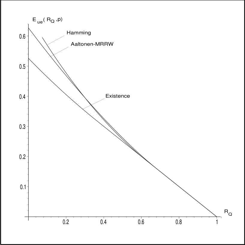
Figure 1: Bounds on $E(R_{Q},p)\!:$ Existence bound, Theorem 1; Aaltonen-MRRW-type bound, Theorem 12; Hamming-type bound, Theorem 14; $p=0.1.$

References

- [1] M. Aaltonen, “Linear programming bounds for tree codes,” IEEE Trans. Info. Theory, vol. 25, no. 1, pp. 85–90, 1979.
- [2] , “A new upper bound on nonbinary block codes,” Discrete Math., vol. 83, no. 2-3, pp.139–160, 1990.
- [3] A. Ashikhmin and A. Barg, “Binomial moments of the distance distribution: Bounds and applications,” IEEE Trans. Info. Theory, vol 45, no. 2, pp. 438-452, 1999.
- [4] A. Ashikhmin and S. Litsyn, “Upper bounds of the size of quantum codes,” IEEE Trans. Info. Theory, vol 45, no. 4, pp.1205-1215, 1999.
- [5] P. Delsarte, “Bounds for unrestricted codes, by linear programming,” Philips Res. Repts, 27 (1972), 272–289.
- [6] , An Algebraic Approach to the Association Schemes of Coding Theory, Philips Research Reports Supplements, No. 10, 1973.
- [7] G. Kalai and N. Linial, “On the distance distribution of codes,” IEEE Trans. Inform. Theory, vol. 42, pp.1467–1472, 1995.
- [8] E. Knill, Non-binary unitary error bases and quantum codes, Los Alamos National Laboratory Report LAUR-96-2717 (1996).
- [9] V. I. Levenshtein, “Bounds on the probability of undetected error,” Problemy Peredachi Informatsii, vol. 13, no. 1, pp. 3–18, 1977.
- [10] , “Krawtchouk polynomials and universal bounds for codes and designs in Hamming spaces,” IEEE Trans. Inform. Theory, vol. 41, no. 3, pp. 1303–1321, 1995.
- [11] S. Litsyn, “New upper bounds on error exponents,” IEEE Trans. Info. Theory, vol. 45, no. 2, pp. 385–398, 1999.
- [12] R. J. McEliece, E. R. Rodemich,H. C. Rumsey, Jr. and L. R. Welch, “New upper bounds on the rate of a code via the Delsarte-MacWilliams Inequalities,”IEEE Trans. Inform. Theory, vol. 23, pp.157–166, 1977.
- [13] F. J. MacWilliams, A. M. Odlyzko, and N. J. A. Sloane, “Self-dual codes over ,” J. of Combin. Theory, Ser. A. vol. 25, pp. 288–318, 1978.
- [14] E. Rains, Nonbinary quantum codes, LANL e-print quant-ph/9703048.
- [15] P.W. Shor and R. Laflamme, “Quantum analog of the MacWilliams identities in classical coding theory,” Phys. Rev. Lett., vol. 78, pp. 1600-1602, 1997.