Loss and heating of particles in small and noisy traps

Abstract

We derive the life time and loss rate for a trapped atom that is coupled to fluctuating fields in the vicinity of a room-temperature metallic and/or dielectric surface. Our results indicate a clear predominance of near field effects over ordinary blackbody radiation. We develop a theoretical framework for both charged ions and neutral atoms with and without spin. Loss processes that are due to a transition to an untrapped internal state are included.
PACS: 03.75.-b Matter waves – 32.80.Lg Mechanical effects of light on atoms and ions – 03.67.-a Quantum information – 05.40.-a Fluctuation phenomena and noise

1 Introduction

Particle traps enjoy great popularity for the preparation and manipulation of coherent matter waves. Prominent applications are the preparation of non-classical states of motion of a single ion Wineland96 , the realization of quantum gates in quasi-one dimensional ion traps Wineland98c , the transfer of atoms through atomic wave guides Ohtsu96b ; Hinds98 ; Haensch98 ; Ertmer98 , and the preparation of quantum-degenerate gases in electromagnetic-solid state hybrid surface traps Ovchinnikov97b ; Mlynek98b . In all these applications, in order to truly benefit from the quantum mechanical effects, coherence of the matter waves and/or their internal degrees of freedom must be maintained as long as possible. Yet, with the physical components which provide the trapping potential being held at room temperatures, the maintenance of coherence seems highly non trivial as the temperature gradient between components and trap center may well exceed $10^{6}{\rm K}/{\rm m}$. A careful study of the particles’ coupling to the trap physical components, and the ensuing heating of the particles is therefore highly desirable.

In the past, the heating of single particles in small traps has been studied by a number of authors Wineland75 ; Lamoreaux97 ; James98 ; Milburn98 ; Knight98 ; Wineland98 . As these studies were mostly performed in the wake of the recent achievements in ion trapping and cooling, the focus in these investigations was on charged particles and their coupling to the surrounding metallic surfaces. In fact, before the advent of laser cooling, this coupling provided the dominant cooling mechanism for an ion cloud, say, as the low-frequency radiation of the ions couples quite efficiently to the lossy currents in the metallic trap components Wineland75 . Yet with the advent of laser cooling, temperatures of a few micro-Kelvin can be reached which are clearly below the components’ temperatures, i.e. the particle-component coupling now leads to heating, and the trap ground state acquires a finite life time. Similar considerations may also be put forward for ultracold neutral atoms trapped in miniaturized traps though the couplings are different: for paramagnetic atoms, e.g., they involve fluctuating magnetic rather than electric fields close to the trap components.

In this paper we derive the life time and loss rate for a trapped particle that is coupled to fluctuating fields in the vicinity of a room-temperature metallic and/or dielectric surface. The theory will be developed for both charged and neutral particles with and without spin, and loss processes that are due to a transition to an untrapped internal state will be included. A detailed derivation of previously published results Henkel99b will also be given.

An essential ingredient of the theory are cross-correlation functions for thermal electric and magnetic fields in a finite geometry. These functions may be simplified for our purposes because the relevant field fluctuation frequencies are much lower than the inverse time for light propagation from the trapped particle to the surface and back. It is hence justified to calculate the fields in the quasi-static limit, neglecting retardation effects. Differently stated, the particle is subject to near field radiation leaking out of the macroscopic trap components. An important consequence is that the near field fluctuations are much stronger than those of the well-known blackbody radiation. This implies larger than expected heating rates, as recently pointed out by Pendry Pendry99b .

The paper is organized as follows: in Sec. 2, the model is presented in terms of a master equation. We identify the relevant heating and loss rates. Sec. 3 is devoted to trapped ion heating. We give the electric field fluctuations above a flat metallic surface. In Sec. 4, heating and loss of a neutral particle with a magnetic moment is studied. The final Sec. 5 gives a summary and outlook. The appendixes contain technical material that is used in the main text.

2 The model: master equation and transition rates

We present here our model for the particle trap and its environment (see fig.1, left part).

Figure 1: Left: trap in front of a flat surface. Right: heating and loss processes.

The model is sufficiently simple to allow for analytical calculations of the relevant heating and loss rates, but also reflects a typical experimental geometry. We consider a single particle bound in a harmonic trap potential whose center is located at a distance $z$ from an infinite flat surface. We consider that this distance is much larger than the size of the particle’s center-of-mass wave function. In this regime, the overlap with the surface is negligible, and the coupling to the surface is mediated via electromagnetic fields. We also focus for simplicity on a single degree of freedom in the harmonic well.

The heating of the particle is described by the transition rate $\Gamma_{0\to 1}$ from the trap ground state $|0\rangle$ to the first excited state $|1\rangle$ (see fig.1, central part). In subsection 2.1, such a ‘heating rate’ is determined from a master equation for the particle’s motion in terms of harmonic-oscillator matrix elements, on the one hand, and the spectral density of a fluctuating force field, on the other.

As a second application, we investigate loss processes in magnetic or optical traps where only a subset of internal states is trapped (see fig.1, right part). This model describes magnetic traps, for example, where only low-field-seeking Zeeman sublevels can be trapped. A loss process occurs when a fluctuating field induces a flip $|i\rangle\to|f\rangle$ of the particle’s internal state. We assume that the particle is then rapidly expelled and lost from the trap. The relevant loss rate $\Gamma_{i\to f}$ is given in subsection 2.2 in terms of internal matrix elements for the particle’s magnetic moment, on the one hand, and the magnetic field fluctuation spectrum, on the other.

2.1 Heating

As mentioned before, we focus on the heating of a single degree of freedom for the trap vibration. The displacement ${\bf x}$ of the particle relative to the trap center ${\bf r}$ is chosen along the unit vector ${\bf n}$ and written in terms of a creation operator $b$. The interaction potential reads

$$V({\bf r},t)=-{\bf x}\cdot{\bf F}({\bf r},t)=-a\left(b+b^{\dagger}\right){\bf n}\cdot{\bf F}({\bf r},t),$$ (1)

where $a=(\hbar/(2M\Omega))^{1/2}$ is the size of the trap ground state ($M$ is the particle mass and $\Omega$ the trap frequency) and ${\bf F}({\bf r},t)$ the force acting on the particle. This force is fluctuating, and it is convenient to use a reduced density matrix description for the particle when the force fluctuations are averaged over. The density matrix $\rho$ evolves according to a master equation that is written in eq.(44) of appendix A.1 for a general coupling. For the Hamiltonian (1), we get the following relaxation dynamics Gardiner

$$\dot{\rho}|_{\rm relax} = -\frac{\gamma_{+}}{2}\left(b^{\dagger}b\rho+\rho b^{\dagger}b-2b\rho b^{\dagger}\right)$$ (2)

$$-\frac{\gamma_{-}}{2}\left(bb^{\dagger}\rho+\rho bb^{\dagger}-2b^{\dagger}\rho b\right).$$

In this equation, the transition rates $\gamma_{\pm}=\gamma({\bf r};\pm\Omega)$ are proportional to the spectral density $S_{F}^{ij}$ of the force fluctuations taken at the trap vibration frequency $\Omega$

$$\gamma({\bf r};\omega)=\frac{a^{2}}{\hbar^{2}}\sum_{ij}n_{i}n_{j}S_{F}^{ij}({\bf r};\omega),$$ (3)

where $S_{F}^{ij}({\bf r};\omega)$ is defined by

$$S_{F}^{ij}({\bf r};\omega)=\int\limits_{-\infty}^{+\infty}\!d\tau\left\langle F_{i}({\bf r},t+\tau)F_{j}({\bf r},t)\right\rangle\,e^{i\omega\tau}.$$ (4)

From the master equation (2), it is easy to obtain rate equations for the populations of the trap levels. For the ground state population $\rho_{00}=\langle 0|\rho|0\rangle$, we get

$$\left.\dot{\rho}_{00}\right|_{\rm relax}=-\gamma_{-}\rho_{00}+\gamma_{+}\rho_{11}.$$ (5)

Note that the transitions towards higher (lower) trap levels occur with a rate equal to $\gamma_{-}$ (to $\gamma_{+}$). In particular, the quantity $\gamma_{-}$ gives the depletion rate of the ground state population. The heating rate we are interested in thus equals

$$\Gamma_{0\to 1}({\bf r})=\gamma_{-}=\frac{a^{2}}{\hbar^{2}}\sum_{ij}n_{i}n_{j}S_{F}^{ij}({\bf r};-\Omega).$$ (6)

Note that the same result may be obtained from Fermi’s Golden Rule, by assuming a mixture of initial states for the fluctuating force field and summing over its final states. In Secs. 3 and 4, the heating rates for trapped ions and spins are computed using (6). The main goal of the calculation is therefore the spectral density of the relevant force (electric or magnetic fields).

Finally, the master equation (2) also allows to describe the decay of the coherences between trap states which is a hazardeous process for quantum bit manipulations. The coherence between the lowest trap levels relaxes according to

$$\left.\dot{\rho}_{01}\right|_{\rm relax}=-\frac{\gamma_{+}+\gamma_{-}}{2}\rho_{01}+\sqrt{2}\gamma_{+}\rho_{12}.$$ (7)

We see that the coherences decay with a similar rate as the populations. This is a consequence of the interaction Hamiltonian (1), and different results are obtained using other couplings or adding explicit phase noise, see, e.g., Refs.Milburn98 ; Knight98 . In the following, we focus on the population dynamics for simplicity.

2.2 Internal state flips

In magnetic or optical traps for neutral particles, the trap potential depends on the internal atomic state (see fig.1, right part). If this state is changed due to fluctuations in the magnetic field, the particle may be subject to an anti-trapping potential and strongly perturbed. The interaction Hamiltonian for spin flips $|i\rangle\to|f\rangle$ is the Zeeman interaction

$$V_{Z}({\bf r},t)=-\mbox{\boldmath$\mu$}\cdot{\bf B}({\bf r},t),$$ (8)

where $\mu$ is the particle’s magnetic moment and ${\bf B}({\bf r},t)$ the fluctuating part of the magnetic field. For this interaction, a master equation similar to (2) may be formulated from the general theory outlined in appendix A.1. This equation is not very instructive, however, if we assume that the particle is lost as soon as it reaches the state $|f\rangle$. In this case, it is sufficient to quote the transition rate $\Gamma_{i\to f}$ obtained from (44)

$$\Gamma_{i\to f}({\bf r})=\sum_{\alpha\beta}\frac{\langle i|\mu_{\alpha}|f\rangle\,\langle f|\mu_{\beta}|i\rangle}{\hbar^{2}}S_{B}^{\alpha\beta}({\bf r};-\omega_{fi}),$$ (9)

where $S_{B}^{\alpha\beta}$ is the magnetic field fluctuation spectrum defined by an expression similar to (4), and $\hbar\omega_{fi}=E_{f}-E_{i}$ the energy difference between initial and final internal states. (We switch to greek subscripts to avoid confusion with the initial state label.) In a magnetic trap, e.g., $|i\rangle$, $|f\rangle$ are magnetic sublevels and the frequency $\omega_{fi}$ a Larmor frequency in the bias field of the trap. In optical traps, we consider the hyperfine components of the atomic ground state, $\omega_{fi}$ is thus the hyperfine splitting.

3 Heating of a trapped charge

In this section, the master equation of the previous section is applied to the most simple situation, that of an electrically charged particle in a harmonic trap Wineland75 ; Lamoreaux97 ; James98 ; Milburn98 ; Knight98 ; Wineland98 . As mentioned in the introduction, the ion is heated up because fluctuating electric fields leak out of the metallic surface nearby. The force in the interaction Hamiltonian (1) is given by the electric field

$${\bf F}({\bf r},t)=q{\bf E}({\bf r},t)$$ (10)

where $q$ is the ion’s charge and ${\bf r}$ the position of the trap center.

3.1 Electric field fluctuations

In the formula (6) for the heating rate, we need the spectral density of the electric field fluctuations $S_{E}^{ij}({\bf r};\omega)$. This quantity is conveniently obtained by making use of the fluctuation-dissipation theorem outlined in appendix A.2. According to this theorem, the field’s spectral density is proportional to the imaginary part of the field’s Green function $G_{ij}({\bf r},{\bf r};\omega)$, multiplied with the Bose-Einstein mean occupation number (eq.(50)). The geometry we have chosen is sufficiently simply to allow the Green function to be calculated analytically Agarwal75a . Recall that the Green function describes the electric field radiated by an oscillating dipole (cf. eq.(49)). This field is the sum of the dipole field in free space plus the field reflected from the surface. The free space field leads to a term $G^{(bb)}_{ij}({\bf r},{\bf r};\omega)$ in the Green function that is actually independent of the trap position ${\bf r}$; it gives the spectral density of the blackbody field (the Planck law)

$$S_{E}^{(bb)ij}({\bf r};\omega) = S_{E}^{(bb)}(\omega)\delta_{ij},$$ (11)

$$S_{E}^{(bb)}(\omega) = \frac{\hbar\omega^{3}}{3\pi\varepsilon_{0}c^{3}(1-e^{-\hbar\omega/T})}$$ (12)

where $T$ is the temperature of the surface (we put the Boltzmann constant $k_{B}=1$).

To calculate the field reflected from the surface, we expand the free space dipole field in plane waves and apply the Fresnel reflection coefficients $r_{s,p}(u)$ for each wave incident on the surface (s and p label the two transverse field polarizations and $u$ is the sine of the angle of incidence). The resulting Green function $G^{(nf)}_{ij}({\bf r},{\bf r};\omega)$ characterizes the modification of the thermal radiation in the near field of the surface. The radiation density is increased with respect to the far field expression (11) because it also contains non-propagating (evanescent) waves. The corresponding spectral density depends only on the distance $z$ to the surface and may be written in the form Agarwal75a

$$S_{E}^{(nf)ij}({\bf r};\omega)=S_{E}^{(bb)}(\omega)g_{ij}(kz)$$ (13)

where the diagonal tensor $g_{ij}$ has the dimensionless elements $g_{xx}=g_{yy}=g_{\|}$ and $g_{zz}=g_{\perp}$ with ($k=|\omega|/c$)

$$g_{\|}(kz) = \frac{3}{4}\mathop{\rm Re}\,\int\limits_{0}^{+\infty}\!\frac{u\,du}{v}e^{2ikzv}\left(r_{s}(u)+(u^{2}-1)r_{p}(u)\right),$$

$$g_{\perp}(kz) = \frac{3}{2}\mathop{\rm Re}\,\int\limits_{0}^{+\infty}\!\frac{u^{3}\,du}{v}e^{2ikzv}r_{p}(u),$$ (14)

$$v = \left\{\begin{array}[]{ll}\sqrt{1-u^{2}},&\quad 0\leq u\leq 1,\\ i\sqrt{u^{2}-1},&\quad u\geq 1.\end{array}\right.$$ (17)

Finally, the relevant Fresnel coefficients are

$$r_{p}(u) = \frac{\varepsilon v-\sqrt{\varepsilon-u^{2}}}{\varepsilon v+\sqrt{\varepsilon-u^{2}}},$$

$$r_{s}(u) = \frac{v-\sqrt{\varepsilon-u^{2}}}{v+\sqrt{\varepsilon-u^{2}}}$$ (18)

where $\varepsilon(\omega)$ is the relative dielectric function of the bulk metal.

For typical trap frequencies the corresponding electromagnetic wavelength is much larger than $z$, so we can restrict our calculations to the quasi-static limit $z\ll{\mathchoice{\hbox{\raise 5.06941pt\hbox to0.0pt{\kern 1.45833pt\vrule width=2.91667pt,height=0.1pt,depth=0.1pt\hss}\hbox{$\displaystyle\lambda$}}}{\hbox{\raise 5.06941pt\hbox to0.0pt{\kern 1.45833pt\vrule width=2.91667pt,height=0.1pt,depth=0.1pt\hss}\hbox{$\textstyle\lambda$}}}{\hbox{\raise 3.54857pt\hbox to0.0pt{\kern 1.02083pt\vrule width=2.04167pt,height=0.1pt,depth=0.1pt\hss}\hbox{$\scriptstyle\lambda$}}}{\hbox{\raise 2.5347pt\hbox to0.0pt{\kern 0.72916pt\vrule width=1.45833pt,height=0.1pt,depth=0.1pt\hss}\hbox{$\scriptscriptstyle\lambda$}}}}$ and find analytical expressions for the tensor elements (17). The details are outlined in appendix B. We have to distinguish between the case of a large and a small skin depth of the conducting material compared to the distance $z$. The skin depth, which is the characteristic length scale on which an electromagnetic wave entering a conducting solid is damped, is given by (for $\omega>0$) Jackson

$$\delta=\frac{1}{k}\sqrt{2\varepsilon_{0}\varrho\omega}$$ (19)

where $\varrho$ is the specific resistance. Since in our frequency regime the dielectric function for a metal is dominated by the zero–frequency pole, it is related to the skin depth by

$$\varepsilon(\omega)\approx\frac{i}{\varepsilon_{0}\varrho\omega}=\frac{2i}{k^{2}\delta^{2}}.$$ (20)

In appendix B.1, we derive approximations for the functions $g_{\|,\perp}(kz)$ in the form of inverse power laws (eqs.(54,56)). Both regimes of large and small skin depth can be covered by the following interpolation formula

$$g_{ij}(kz)=\frac{3\delta^{2}}{8kz^{3}}\left(s_{ij}+\delta_{ij}\frac{z}{\delta}\right)$$ (21)

where $s_{ij}$ is a diagonal tensor with the elements $s_{xx}=s_{yy}=\frac{1}{2}$, $s_{zz}=1$. Thus we arrive at a final expression for the electric field spectrum, applying the high temperature limit of the Planck law (12):

$$S_{E}^{(nf)ij}({\bf r};\omega)=\frac{T\varrho}{4\pi z^{3}}\left(s_{ij}+\delta_{ij}\frac{z}{\delta(|\omega|)}\right).$$ (22)

We note that in the case of a short distance, the parallel and perpendicular tensor elements both show a $1/z^{3}$-dependence and differ by a factor of 2, whereas for larger distances the tensor elements are equal and show a $1/z^{2}$-behavior.

The $1/z^{3}$ power law of the regime $z\ll\delta$ may be understood in terms of image theory: the electrostatic dipole field varies precisely as $1/r^{3}$ and its reflection from the surface is characterized by the factor $(\varepsilon-1)/(\varepsilon+1)\approx 1+i(k\delta)^{2}$. The imaginary part of the reflected field thus reproduces (21). This is the regime discussed in Ref.Henkel99b . It is interesting to note that for a larger distance $z\gg\delta$, the field fluctuations are enhanced with respect to the electrostatic regime (see fig. 2). This is due to the fact that the dipole field is more efficiently damped in the conductor because the exponential decay in the skin layer quenches the algebraic penetration of the field.

For completeness, we also mention the limiting case of a perfectly conducting surface ($\varepsilon\to\infty$) whose skin depth $\delta$ vanishes. The previous asymptotic expansion does not cover this case. The coefficients $g_{\|,\perp}(kz)$ given in the appendix B, eq.(57), show damped oscillations with a period equal to the wavelength. In the short-distance limit $z\ll{\mathchoice{\hbox{\raise 5.06941pt\hbox to0.0pt{\kern 1.45833pt\vrule width=2.91667pt,height=0.1pt,depth=0.1pt\hss}\hbox{$\displaystyle\lambda$}}}{\hbox{\raise 5.06941pt\hbox to0.0pt{\kern 1.45833pt\vrule width=2.91667pt,height=0.1pt,depth=0.1pt\hss}\hbox{$\textstyle\lambda$}}}{\hbox{\raise 3.54857pt\hbox to0.0pt{\kern 1.02083pt\vrule width=2.04167pt,height=0.1pt,depth=0.1pt\hss}\hbox{$\scriptstyle\lambda$}}}{\hbox{\raise 2.5347pt\hbox to0.0pt{\kern 0.72916pt\vrule width=1.45833pt,height=0.1pt,depth=0.1pt\hss}\hbox{$\scriptscriptstyle\lambda$}}}}$, we get $g_{\|}(kz)\to-1$ and $g_{\perp}(kz)\to 1$, the divergence at $z\to 0$ thus disappears. The electric field fluctuations are essentially those of the free space blackbody spectrum, with a minor modification due to the boundary conditions.

3.2 Heating rate

We plot in fig. 2 the heating rate (6) for an ion (trap frequency $\Omega/2\pi=1\,$MHz) above a copper surface.

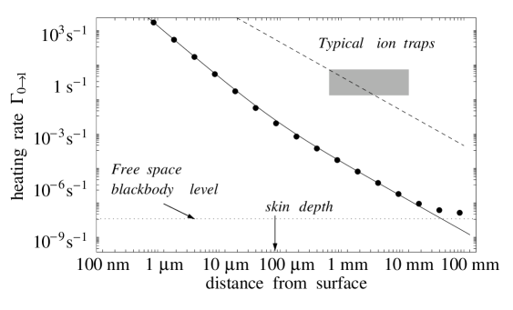
Figure 2: Heating rate for a trapped ion. Dots: coupling to electric proximity fields, computed from (17). The solid line is obtained using the asymptotic formula (21). Dashed line: coupling to thermal voltage fluctuations.
Parameters: trap frequency $\Omega/2\pi=1\,$MHz, copper substrate with $\varrho=1.7\times 10^{-6}\,{\rm\Omega\,cm}$ at $T=300\,{\rm K}$. The ion mass is $M=40\,{\rm amu}$, and its charge $q=e$. The trap axis is perpendicular to the surface, ${\bf n}={\bf e}_{z}$. The thermal voltage fluctuations are characterized by a circuit resistance $1\,{\rm\Omega}$ Lamoreaux97 . The endcaps are separated by twice the ion-surface distance. Size and inverse lifetimes of typical ion traps are indicated by the shaded rectangle Wineland96 ; Blatt99p ; Peik99p .

The dots are based on an exact (numerical) evaluation of the $g$-coefficients (17), while the solid line uses the interpolation (21). The change in the power law at the skin depth is clearly visible. Note the marked increase of the field fluctuations compared to the free space blackbody level (dotted line). Also shown is the estimate given by Lamoreaux Lamoreaux97 who modeled the trap in terms of a resistively damped capacitor with a thermally fluctuating voltage (Johnson noise). Wineland et al. Wineland98 pointed out that realistic estimates for the corresponding resistance actually give smaller heating rates. Our results suggest that the miniaturization of ion traps down to $\mu$m sizes entails difficulties to maintain long coherent storage times, unless all physical components are cooled down.

4 Trapped spin coupling to magnetic fields

In this section, we turn to traps for neutral particles and consider the Zeeman coupling (8) of the atomic magnetic moment to a fluctuating magnetic field. In magnetic and optical traps, this coupling may induce a spin flip to a non-trapped state (magnetic sublevel or hyperfine state). This implies a nonzero loss rate from the trap that we calculate in subsection 4.1. On the other hand, the Zeeman interaction also exerts a force proportional to the gradient of the magnetic field. If this force fluctuates, it does not necessarily flip the atomic spin, but excites the atom into a higher trap level. The corresponding heating rate is the subject of subsection 4.2.

4.1 Spin flips

4.1.1 Magnetic field correlations.

We first compute the magnetic field fluctuations in the vicinity of the solid surface. By analogy to the ion case, we use the fluctuation-dissipation theorem (50) and determine the Green tensor for the magnetic field. In fact, the calculation is very similar to that for the electric field: starting from the field radiated in free space, we expand it in spatial Fourier components and compute for each plane wave the reflection at the solid surface. It turns out that the Fresnel coefficients for the magnetic field are identical to those for electric fields, except that one has to exchange the s- and p-polarizations. We thus get the following near-field correction to the magnetic field fluctuation spectrum

$$S_{B}^{(nf)ij}({\bf r};\omega)=\frac{S_{E}^{(bb)}(\omega)}{c^{2}}h_{ij}\!\left(kz\right).$$ (23)

Similar to (13), $h_{ij}$ is a dimensionless and diagonal tensor with elements

$$h_{\|}(kz) = \frac{3}{4}\mathop{\rm Re}\,\int\limits_{0}^{+\infty}\!\frac{u\,du}{v}e^{2ikzv}\left(r_{p}(u)+(u^{2}-1)r_{s}(u)\right),$$

$$h_{\perp}(kz) = \frac{3}{2}\mathop{\rm Re}\,\int\limits_{0}^{+\infty}\!\frac{u^{3}\,du}{v}e^{2ikzv}r_{s}(u).$$ (24)

For experimentally relevant parameters, the magnetic fields at the resonance frequency have a wavelength (at least some cm) much longer than the size of the trap. This implies again that we need the short-distance asymptotics $z\ll{\mathchoice{\hbox{\raise 5.06941pt\hbox to0.0pt{\kern 1.45833pt\vrule width=2.91667pt,height=0.1pt,depth=0.1pt\hss}\hbox{$\displaystyle\lambda$}}}{\hbox{\raise 5.06941pt\hbox to0.0pt{\kern 1.45833pt\vrule width=2.91667pt,height=0.1pt,depth=0.1pt\hss}\hbox{$\textstyle\lambda$}}}{\hbox{\raise 3.54857pt\hbox to0.0pt{\kern 1.02083pt\vrule width=2.04167pt,height=0.1pt,depth=0.1pt\hss}\hbox{$\scriptstyle\lambda$}}}{\hbox{\raise 2.5347pt\hbox to0.0pt{\kern 0.72916pt\vrule width=1.45833pt,height=0.1pt,depth=0.1pt\hss}\hbox{$\scriptscriptstyle\lambda$}}}}$ of (23). A calculation outlined in appendix B.2 gives the following interpolation formula that covers both regimes of a large and small skin depth

$$h_{ij}(kz)=\frac{3s_{ij}}{8k^{3}\delta^{2}z}\left(1+\frac{2z^{3}}{3\delta^{3}}\right)^{-1}$$ (25)

where $s_{ij}$ is the diagonal tensor introduced in (21). The magnetic field spectrum (23) thus equals in the high-temperature limit

$$S_{B}^{(nf)ij}({\bf r};\omega)=\frac{\mu_{0}^{2}T}{16\pi\varrho}\frac{s_{ij}}{z}\left(1+\frac{2z^{3}}{3\delta^{3}(|\omega|)}\right)^{-1}.$$ (26)

Note the different exponents for the distance dependence compared to the electric field fluctuations (22).

If the trap distance is small compared to the skin depth, we recover the magnetic field spectrum given in eq.(10) of Henkel99b , apart from the fact that the parallel tensor components ($s_{xx}$, $s_{yy}$) differ. This difference is due to the fact that the calculation of Henkel99b uses the Biot-Savart law to get the magnetic field from a statistical model of polarization currents in the solid. This approach is valid for stationary currents only, and a difficulty appears at the surface because the model for the currents is not divergence-free there. Therefore, while the magnetic field perpendicular to the surface is correctly described, the parallel components are overestimated.

4.1.2 Internal matrix elements.

In order to compute the spin flip loss rate we have to evaluate matrix elements of the total magnetic moment operator as indicated in (9). This operator is in general given by

$${\bf\mu}=-\mu_{B}\left(g_{L}{\bf L}+g_{S}{\bf S}-g_{I}\frac{m_{e}}{m_{p}}{\bf I}\right),$$ (27)

with $\mu_{B}$ the Bohr magneton, ${\bf L}$ the total orbital angular momentum operator, ${\bf S}$ the electronic spin operator, ${\bf I}$ the nuclear spin operator and $g_{L}$, $g_{S}$ and $g_{I}$ the corresponding $g$-factors. Since the proton mass $m_{p}$ is larger than the electron mass $m_{e}$ by three orders of magnitude, we can neglect the contribution of the nuclear magnetic moment. Furthermore, the reasonable restriction to an atomic ground state with $L=0$ reduces the problem to the calculation of matrix elements of solely the spin operator. Together with the fact that the tensor $h_{ij}$ in (25) for the magnetic field correlations is diagonal, we can focus on terms of the form

$$\left|\left\langle f\right|\mu_{\alpha}\left|i\right\rangle\right|^{2}=\mu_{B}^{2}g_{S}^{2}\left|\left\langle f\right|S_{\alpha}\left|i\right\rangle\right|^{2}.$$ (28)

In the following we will restrict ourselves to two extreme cases: the coupling between two Zeeman sublevels in the presence of an external magnetic field and the coupling between two hyperfine ground states without external fields applied. The former case is e.g. realized in a magnetic trap, whereas the latter corresponds to optical traps.

In the case of a magnetic trap the trapped atom is subject to a constant magnetic field with strength $B_{0}$ in the center of the trap, assuming the atom is not moving. The magnetic sublevels are split due to the Zeeman effect by the Larmor frequency $\omega_{L}=g_{S}\mu_{B}B_{0}/\hbar$. (We focus on a vanishing nuclear spin for simplicity.) Without loss of generality we can assume the magnetic field to be lying within the $xz$-plane, since the diagonal tensor in (25) has the symmetry property $h_{xx}=h_{yy}$. If the magnetic field forms an angle $\theta$ with respect to the $z$-axis, we denote by $|m\rangle_{\theta}$ the basis states with quantization axis parallel to the magnetic field (the ‘trap basis’). Rewriting (28) leaves us to calculate matrix elements of the form

$$\left|\left\langle f\right|\mu_{\alpha}\left|i\right\rangle\right|^{2}=\mu_{B}^{2}g_{S}^{2}\left|{}_{\theta}\langle m_{f}|S_{\alpha}|m_{i}\rangle_{\theta}\right|^{2}.$$ (29)

These elements are evaluated by expanding the spin vector components in a rotated coordinate system (denoted by the prime) adapted to the trap basis. The result is the following:

$${}_{\theta}\langle m_{f}|S_{x}|m_{i}\rangle_{\theta} = \left({}_{\theta}\langle m_{f}|S_{+}^{\prime}|m_{i}\rangle_{\theta}+{}_{\theta}\langle m_{f}|S_{-}^{\prime}|m_{i}\rangle_{\theta}\right)\frac{\cos{\theta}}{2}$$

$$+ {}_{\theta}\langle m_{f}|S_{3}^{\prime}|m_{i}\rangle_{\theta}\sin{\theta},$$

$${}_{\theta}\langle m_{f}|S_{y}|m_{i}\rangle_{\theta} = \frac{i}{2}\left({}_{\theta}\langle m_{f}|S_{-}^{\prime}|m_{i}\rangle_{\theta}-{}_{\theta}\langle m_{f}|S_{+}^{\prime}|m_{i}\rangle_{\theta}\right),$$

$${}_{\theta}\langle m_{f}|S_{3}|m_{i}\rangle_{\theta} = \left({}_{\theta}\langle m_{f}|S_{+}^{\prime}|m_{i}\rangle_{\theta}+{}_{\theta}\langle m_{f}|S_{-}^{\prime}|m_{i}\rangle_{\theta}\right)\frac{{-\sin{\theta}}}{2}$$ (30)

$$+ {}_{\theta}\langle m_{f}|S_{3}^{\prime}|m_{i}\rangle_{\theta}\cos{\theta}$$

where $S_{3}^{\prime}$ is the $z$-component of the spin operator and $S_{+}^{\prime}$, $S_{-}^{\prime}$ correspond to raising resp. lowering operators in the trap basis, whose action is known Sakurai . In the case of an electronic spin $S=1/2$, the trapped (untrapped) level is the $|m_{i}\rangle_{\theta}=|{-1/2}\rangle_{\theta}$ ($|m_{f}\rangle_{\theta}=|1/2\rangle_{\theta}$) Zeeman sublevel, respectively. The matrix elements (30) then become

$${}_{\theta}\langle 1/2|S_{x}|{-1/2}\rangle_{\theta} = \frac{\cos{\theta}}{2},$$

$${}_{\theta}\langle 1/2|S_{y}|{-1/2}\rangle_{\theta} = -\frac{i}{2},$$

$${}_{\theta}\langle 1/2|S_{z}|{-1/2}\rangle_{\theta} = -\frac{\sin{\theta}}{2}.$$ (31)

With this result, we can compute the magnetic loss rate (36) below.

In the case of an optical trap we have to take into account that the nuclear spin couples to the electronic spin, ${\bf F}={\bf S}+{\bf I}$, and causes the ground state to split into hyperfine levels, separated by a frequency $\omega_{HF}$. We are now interested in the transition probability from one hyperfine ground state to another. Thus, for this case we can write (28) as

$$\left|\left\langle f\right|\mu_{\alpha}\left|i\right\rangle\right|^{2}=\mu_{B}^{2}g_{S}^{2}\left|\left\langle F_{f}\right|S_{\alpha}\left|F_{i}\right\rangle\right|^{2}$$ (32)

A transition from one hyperfine ground state to another can take place between different magnetic sublevels. Thus we first have to calculate the transition rate between two of these states. This is done by expanding the basis states in the uncoupled basis, choosing the quantization axis taken along the $z$-axis:

$$\left|Fm\right\rangle=\sum_{m_{S},m_{I}}C^{m_{S}{}m_{I}}_{F{}m}\left|m_{S}m_{I}\right\rangle$$ (33)

where $C^{m_{S}{}m_{I}}_{F{}m}$ are the Clebsch–Gordan coefficients. The matrix element between two hyperfine magnetic levels is then

$$\left\langle F_{f}m_{f}\right|S_{\alpha}\left|F_{i}m_{i}\right\rangle$$

$$=\sum_{m_{S},m_{S}^{\prime},m_{I}}C^{m_{S}^{\prime}{}m_{I}}_{F_{f}{}m_{f}}C^{m_{S}{}m_{I}}_{F_{i}{}m_{i}}\left\langle m_{S}^{\prime}\right|S_{\alpha}\left|m_{S}\right\rangle.$$ (34)

Note that the nuclear spin does not flip in the transition. Again the action of $S_{\alpha}$ onto the electronic spin states $|m_{S}\rangle$ is well–known in (34). We obtain an effective transition rate between the two hyperfine manifolds by summing the rates over all final $m_{f}$-levels and taking the average over the initial $m_{i}$-levels. This gives the following result for the hyperfine matrix element (32)

$$\left|\left\langle F_{f}\right|S_{\alpha}\left|F_{i}\right\rangle\right|^{2}=\frac{1}{2F_{i}+1}\sum_{m_{f},m_{i}}\left|\left\langle F_{f}m_{f}\right|S_{\alpha}\left|F_{i}m_{i}\right\rangle\right|^{2}.$$ (35)

We finally note that this calculation assumes that the frequencies for the transitions $|F_{i}m_{i}\rangle\to|F_{f}m_{f}\rangle$ are all equal to the hyperfine splitting $\omega_{HF}$. This is a good approximation if $\hbar\omega_{HF}$ is large compared to the optical trap potential (that may lift the degeneracy of the hyperfine states even without a static magnetic field).

4.1.3 Loss rate.

Combining the matrix elements (28) for the magnetic moment, the magnetic field spectrum (26) and eq.(9), we get the following loss rate for a magnetic trap

$$\Gamma_{i\to f}({\bf r})=\frac{\mu_{B}^{2}g_{S}^{2}\omega_{L}^{2}T}{3\pi\varepsilon_{0}\hbar^{2}c^{5}}\sum_{\alpha}(h_{\alpha\alpha}(kz)+1)\left|\langle f|S_{\alpha}|i\rangle\right|^{2}.$$ (36)

For the case of an electronic spin $S=1/2$ and no nuclear spin we can use the matrix elements from (31) and obtain

$$\Gamma_{-\frac{1}{2}\to\frac{1}{2}}({\bf r}) = \frac{\mu_{B}^{2}g_{S}^{2}\omega_{L}^{2}T}{12\pi\varepsilon_{0}\hbar^{2}c^{5}}\left\{(h_{\parallel}(kz)+1)(1+\cos^{2}{\theta})+{}\right.$$ (37)

$$\qquad\left.{}+(h_{\perp}(kz)+1)\sin^{2}{\theta}\right\}.$$

This loss rate is plotted in fig. 3 for two different Larmor frequencies $\omega_{L}$, with the trap bias field chosen parallel to the surface ($\theta=\pi/2$).

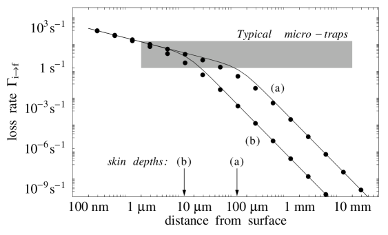
Figure 3: Loss rates in a magnetic trap above a copper surface. Dots (solid lines): results based on (24) (on the asymptotic interpolation (25)). Results for two different Larmor frequencies $\omega_{L}/2\pi=1\,$MHz (curve a) and $100\,$MHz (curve b) are shown. The arrows mark the corresponding skin depths. The shaded area indicates experimental data obtained in Konstanz and Heidelberg Ovchinnikov97b ; Mlynek98b .
Parameters: spin $S=1/2$, magnetic bias field aligned parallel to the surface. The loss rate due to the blackbody field (the prefactor in (37)) is about $10^{-13}\,{\rm s}^{-1}$ at $100\,$MHz (not shown).

We see that quite large loss rates occur if the trap center approaches the surface down to a few micrometers. Again, miniaturized traps have to face the influence of larger noise fields.

In fig. 4, we plot the loss rates obtained from the effective matrix element (35) for hyperfine-changing transitions. The data are calculated for the lower ground states of trapped ⁸⁵Rb and ¹³³Cs. One observes that these rates are much smaller than those for magnetic traps. It is interesting that this reduction is due to the skin effect: indeed, the magnetic field fluctuations (26) in the intermediate-distance regime $\delta\ll z\ll{\mathchoice{\hbox{\raise 5.06941pt\hbox to0.0pt{\kern 1.45833pt\vrule width=2.91667pt,height=0.1pt,depth=0.1pt\hss}\hbox{$\displaystyle\lambda$}}}{\hbox{\raise 5.06941pt\hbox to0.0pt{\kern 1.45833pt\vrule width=2.91667pt,height=0.1pt,depth=0.1pt\hss}\hbox{$\textstyle\lambda$}}}{\hbox{\raise 3.54857pt\hbox to0.0pt{\kern 1.02083pt\vrule width=2.04167pt,height=0.1pt,depth=0.1pt\hss}\hbox{$\scriptstyle\lambda$}}}{\hbox{\raise 2.5347pt\hbox to0.0pt{\kern 0.72916pt\vrule width=1.45833pt,height=0.1pt,depth=0.1pt\hss}\hbox{$\scriptscriptstyle\lambda$}}}}$ are proportional to $\delta^{3}\propto\omega^{-3/2}$. Larger transition frequencies thus lead to smaller loss rates.

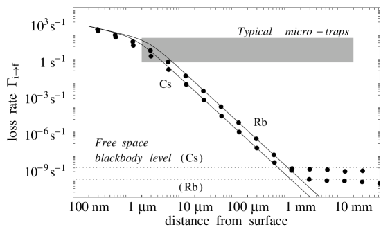
Figure 4: Loss rates due to hyperfine-changing transitions in an optical trap above a copper surface. Dots (solid lines): results based on (24) (on the asymptotic interpolation (25)). Results for two different atoms are shown: ⁸⁵Rb ($I=5/2$, $\omega_{HF}/2\pi=3.04\,$GHz, transition $F_{i}=2\to 3=F_{f}$) and ¹³³Cs ($I=7/2$, $\omega_{HF}/2\pi=9.193\,$GHz, transition $F_{i}=3\to 4=F_{f}$). The horizontal dotted line marks the corresponding loss rates in the free space blackbody field.

4.2 Heating of the c.m. motion

This case is treated by analogy to the trapped ion. The Zeeman interaction (8) gives the following magnetic force

$${\bf F}_{Z}({\bf r},t)=\nabla\left(\mbox{\boldmath$\mu$}\cdot{\bf B}({\bf r},t)\right)$$ (38)

that couples to the displacement of the particle from its equilibrium position. The matrix elements for the displacement are that of a 1D harmonic oscillator and are given in subsection 2.1. We are left with the calculation of the magnetic force’s spectral density. To this end, recall the identity

$$\langle F_{Zi}({\bf r},t^{\prime})F_{Zj}({\bf r},t)\rangle$$

$$=\left.\frac{\partial}{\partial r_{1i}}\frac{\partial}{\partial r_{2j}}\langle V_{Z}({\bf r}_{1},t^{\prime})V_{Z}({\bf r}_{2},t^{\prime})\rangle\right|_{{\bf r}_{1}={\bf r}_{2}={\bf r}}.$$ (39)

The relevant information is thus contained in the cross correlation function for the magnetic field at two different positions ${\bf r}_{1,2}$. From the fluctuation-dissipation theorem (appendix A.2), this correlation function is proportional to the Green function $H_{ij}({\bf r}_{1},{\bf r}_{2};\omega)$ for the magnetic field. To simplify the calculation, we focus on a trap with an axis ${\bf n}$ perpendicular to the surface. According to (6), we then only need the $zz$-component of the force fluctuation tensor. In the identity (39), it is thus sufficient to take two positions ${\bf r}_{1,2}=({\bf R},z_{1,2})$ that differ only in the vertical coordinate (${\bf R}=(x,y)$ denotes the coordinates parallel to the surface). It may now be shown that the surface-dependent part $H^{(nf)}_{ij}({\bf r}_{1},{\bf r}_{2};\omega)$ of the Green tensor depends only on the average distance $\bar{z}=(z_{1}+z_{2})/2$ and the lateral separation ${\bf R}_{2}-{\bf R}_{1}$ Agarwal75a . This is clear, e.g., from image theory. Since ${\bf R}_{1}={\bf R}_{2}$ for our special case, we may write

$$H^{(nf)}_{ij}({\bf R},z_{1},{\bf R},z_{2};\omega)=H^{(nf)}_{ij}({\bf R},\bar{z},{\bf R},\bar{z};\omega)$$ (40)

where the right-hand side is the Green function taken at identical positions that has been calculated in subsection 4.1.1.

We now use the results (58, 59) for the magnetic correlation tensor (app. B.2), write $z=(z_{1}+z_{2})/2$ and differentiate with respect to $z_{1,2}$. All told, both asymptotic regimes of small and large skin depth are described by the interpolation formula

$$S_{F_{Z}}^{zz}({\bf r};\omega)=\frac{\mu_{0}^{2}T}{64\pi\varrho}\frac{\langle i|\mbox{\boldmath$\mu$}^{2}+\mu_{3}^{2}|i\rangle}{z^{3}}\left(1+\frac{z^{3}}{15\delta^{3}}\right)^{-1}.$$ (41)

This spectrum is already summed over all final Zeeman states, assuming that all of them are trapped. The average for the magnetic moment is taken in the initial state. For an atom with $L=0,S=1/2$ in the ground state, it equals $g_{S}^{2}\mu_{B}^{2}\approx 4\mu_{B}^{2}$ where $\mu_{B}$ is the Bohr magneton.

If the trap distance is small compared to the skin depth, we recover the expression (11) of Henkel99b for the heating rate

$$\Gamma_{0\to 1}({\bf r})=\frac{\mu_{0}^{2}T\mu^{2}_{B}g_{S}^{2}}{64\pi\hbar\Omega M\varrho\,z^{3}},$$ (42)

apart from different weights for the parallel and perpendicular spin components. This is due to the different magnetic field correlation tensor (26) that has already been discussed above.

In fig. 5, we plot the heating rate $\Gamma_{0\to 1}$ obtained from the magnetic fluctuation spectrum (41) for a typical trap above both a copper and a glass surface. The heating rate above glass is much smaller because glass is a poor conductor. For a copper substrate, note the crossover when the distance becomes larger than the skin depth. A remarkable result is the large value of the heating rate for small traps (dimensions below the $\mu$m range).

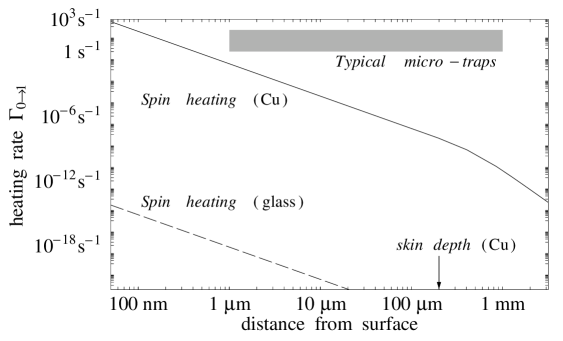
Figure 5: Heating rate for a trapped spin above copper and glass substrates.
Parameters: trap frequency $\Omega/2\pi=100\,{\rm kHz}$, $M=40\,{\rm amu}$, magnetic moment $\mu=\mu_{B}=$ 1 Bohr magneton, spin $S=1/2$. The heating rate due to the magnetic blackbody field (not shown) is about $10^{-39}\,{\rm s}^{-1}$. For the glass substrate, a dielectric constant with $\mathop{\rm Re}\,\varepsilon=5$ and a specific resistance $\varrho=10^{11}{\rm\Omega}\,{\rm cm}$ are taken. These values are used in the short-distance asymptotics (58) to compute the magnetic field fluctuations.

5 Summary and outlook

To summarize, we have developed a theoretical framework for the systematic investigation of the heating and concomitant loss of coherence in small particle traps. Our results indicate a clear predominance of near field effects over ordinary (free space) blackbody radiation. They establish upper bounds for life times in a variety of experimentally relevant types of traps.

The present model is restricted to particle motion in a single dimension, and the extension to a three-dimensional trap geometry is an obvious step for future work. A theory beyond the rate equations discussed here could include noise-induced shifts of the particle’s energy levels. Finally, still other interactions might be considered for neutral atoms. The coupling to electric fields via the polarizability tensor is currently under investigation.

Acknowledgments.

C. H. would like to thank Rémi Carminati, Jean-Jacques Greffet, Karl Joulain, and Stefan Scheel for sharing their deep understanding of electromagnetic near-field spectra. We are indebted to John B. Pendry, Ekkehard Peik, and Ferdinand Schmidt-Kaler for communicating results of previously unpublished work. Travel costs have been covered by Laboratoire d’Energétique Moléculaire et Macroscopique, Combustion of Ecole Centrale Paris, Châtenay-Malabry, France. This work has been supported by a research grant awarded to C. H. by the Deutsche Forschungsgemeinschaft.

Appendix A Statistical tools

A.1 Master equations

We outline here a general master equation Agarwal75a that describes the reduced dynamics of a system coupled to a reservoir. The coupling Hamiltonian is given in terms of an arbitrary system operator ${\bf s}$, a fluctuating force ${\bf F}({\bf r},t)$, and a coupling constant $g$

$$V({\bf r},t)=-g\,{\bf s}\cdot{\bf F}({\bf r},t).$$ (43)

Throughout this paper, the parameter ${\bf r}$ denotes the trap center position. For a trapped ion, e.g., the system operator ${\bf s}$ would describe the displacement of the ion from the trap center, see eq.(1). In the Markov limit and ignoring reservoir-induced level shifts, the relaxation dynamics of the reduced system density matrix $\rho$ is

$$\dot{\rho}|_{\rm relax} = -\frac{g^{2}}{\hbar^{2}}\sum_{ij}\frac{S_{F}^{ij}({\bf r};\omega)}{2}\left(s_{i}^{(-)}s_{j}^{(+)}\rho+\rho s_{i}^{(-)}s_{j}^{(+)}\right.$$ (44)

$$\quad\left.-2s_{j}^{(+)}\rho s_{i}^{(-)}\right)$$

$$-\frac{g^{2}}{\hbar^{2}}\sum_{ij}\frac{S_{F}^{ij}({\bf r};-\omega)}{2}\left(s_{i}^{(+)}s_{j}^{(-)}\rho+\rho s_{i}^{(+)}s_{j}^{(-)}\right.$$

$$\quad\left.-2s_{j}^{(-)}\rho s_{i}^{(+)}\right)$$

where the ${\bf s}^{(\pm)}$ is the positive (negative) frequency part of the system operator. More precisely, the free system evolution in the Heisenberg picture is given by

$${\bf s}(t)={\bf s}^{(+)}e^{-i\omega t}+{\bf s}^{(-)}e^{i\omega t}$$ (45)

where $\hbar\omega\,(>0)$ is the energy difference between two adjacent system states. The spectral density in (44) is defined by (cf. eq.(4))

$$S_{F}^{ij}({\bf r};\omega)=\int\limits_{-\infty}^{+\infty}\!d\tau\left\langle F_{i}({\bf r},t+\tau)F_{j}({\bf r},t)\right\rangle\,e^{i\omega\tau}.$$ (46)

The master equation (44) allows to derive rate equations similar to (5), and these show that the rates proportional to $S_{F}^{ij}({\bf r};+\omega)$ govern spontaneous and stimulated decay processes, while excitation processes are proportional to $S_{F}^{ij}({\bf r};-\omega)$. The latter correlation function is thus relevant for our heating problem.

A.2 Fluctuation–dissipation theorem

In a reservoir at thermal equilibrium, there is a relation between the cross correlation tensor for the field fluctuations and the field’s Green tensor Agarwal75a . This relation also holds for correlations taken at different positions in space, that we have to compute in subsection 4.2. For a force field ${\bf F}({\bf r},t)$, the cross correlation tensor is defined by generalizing (46)

$$S_{F}^{ij}({\bf r}_{1},{\bf r}_{2};\omega)=\int\limits_{-\infty}^{+\infty}\!d\tau\left\langle F_{i}({\bf r}_{1},t+\tau)F_{j}({\bf r}_{2},t)\right\rangle\,e^{i\omega\tau}.$$ (47)

The Green function is defined as the force field created by a classical monochromatic, localized disturbance ${\bf a}$ at ${\bf r}_{0}$ (e.g. the electric field of an oscillating point dipole). The interaction Hamiltonian density is

$$-e^{-i\omega t}\delta({\bf r}-{\bf r}_{0}){\bf a}\cdot{\bf F}({\bf r},t).$$ (48)

In thermal equilibrium, the average linear response to this source is a harmonic field $\langle{\bf F}({\bf r},t;{\bf r}_{0})\rangle$ that depends parametrically on the source position ${\bf r}_{0}$ and is proportional to the displacement ${\bf a}$. The Green function is the corresponding proportionality factor

$$\langle F_{i}({\bf r},t;{\bf r}_{0})\rangle=e^{-i\omega t}\sum_{j}G_{ij}({\bf r},{\bf r}_{0};\omega)a_{j}.$$ (49)

(The averaging $\langle\cdots\rangle$ removes the oscillations of the free field.) The fluctuation-dissipation theorem now states Agarwal75a

$$S_{F}^{ij}({\bf r}_{1},{\bf r}_{2};\omega)=\frac{2\hbar}{1-e^{-\hbar\omega/T}}\mathop{\rm Im}\,G_{ij}({\bf r}_{1},{\bf r}_{2};\omega).$$ (50)

Note that in terms of the mean thermal occupation number $\bar{n}_{\rm th}=1/(e^{\hbar\omega/T}-1)$, one has (for $\omega>0$)

$$S_{F}^{ij}({\bf r}_{1},{\bf r}_{2};\omega) = 2\hbar\left(\bar{n}_{\rm th}+1\right)\mathop{\rm Im}\,G_{ij}({\bf r}_{1},{\bf r}_{2};\omega),$$ (51)

$$S_{F}^{ij}({\bf r}_{1},{\bf r}_{2};-\omega) = 2\hbar\bar{n}_{\rm th}\mathop{\rm Im}\,G_{ij}({\bf r}_{1},{\bf r}_{2};\omega).$$ (52)

At zero temperature, $\bar{n}_{\rm th}=0$, and only the first line survives. The relaxation dynamics is then entirely due to spontaneous decay, induced by the vacuum fluctuations of the force field. Heating processes are suppressed. At high temperature, $\bar{n}_{\rm th}\gg 1$, the fluctuation spectrum becomes independent of the sign of $\omega$. In the master equation, decay and excitation rates are then nearly the same.

Appendix B Asymptotic expansion of electromagnetic field spectra

B.1 Electric field

We outline here the asymptotic expansion for the coefficients $g_{\|,\perp}(kz)$ that characterize the electric field fluctuations (13) in the near field $kz\ll 1$ of the surface.

The inspection of the integrals (17) shows that the exponential $e^{2ikzv}\approx e^{-2kzu}$ decreases on a large scale $u\sim 1/(kz)\gg 1$. On the other hand, the other factors in the integrands increase as powers of $u$. The value of the integral is thus dominated by values $u\sim u_{\max}$ around the maximum $u_{\max}\sim 1/(kz)\gg 1$. It is therefore accurate to use asymptotic expansions of the Fresnel coefficients for large $u\gg 1$. The asymptotic form of the coefficients depends, however, on whether $u^{2}_{\max}$ is smaller or larger than the magnitude $|\varepsilon|$ of the dielectric constant. These two regimes are discussed in the following. Their physical significance follows from the relation (20) between $\varepsilon$ and the skin depth $\delta$.

The limit $1\ll|\varepsilon|^{1/2}\ll u$ corresponds to a distance small compared to the skin depth, $z\ll\delta\ll{\mathchoice{\hbox{\raise 5.06941pt\hbox to0.0pt{\kern 1.45833pt\vrule width=2.91667pt,height=0.1pt,depth=0.1pt\hss}\hbox{$\displaystyle\lambda$}}}{\hbox{\raise 5.06941pt\hbox to0.0pt{\kern 1.45833pt\vrule width=2.91667pt,height=0.1pt,depth=0.1pt\hss}\hbox{$\textstyle\lambda$}}}{\hbox{\raise 3.54857pt\hbox to0.0pt{\kern 1.02083pt\vrule width=2.04167pt,height=0.1pt,depth=0.1pt\hss}\hbox{$\scriptstyle\lambda$}}}{\hbox{\raise 2.5347pt\hbox to0.0pt{\kern 0.72916pt\vrule width=1.45833pt,height=0.1pt,depth=0.1pt\hss}\hbox{$\scriptscriptstyle\lambda$}}}}$. In this regime, we get the following asymptotic expressions for the Fresnel coefficients (18)

$$r_{p}(u)\to\frac{\varepsilon-1}{\varepsilon+1},$$

$$r_{s}(u)\to\frac{\varepsilon-1}{4u^{2}}.$$ (53)

The integrals (17) for the tensor elements are then evaluated to

$$g_{\|}(kz)\approx\frac{3}{16(kz)^{3}}\mathop{\rm Im}\,\frac{\varepsilon-1}{\varepsilon+1}\approx\frac{3\delta^{2}}{16kz^{3}},$$

$$g_{\perp}(kz)\approx 2g_{\|}(kz).$$ (54)

In the opposite limit of a small skin depth, i.e. $\delta\ll z\ll{\mathchoice{\hbox{\raise 5.06941pt\hbox to0.0pt{\kern 1.45833pt\vrule width=2.91667pt,height=0.1pt,depth=0.1pt\hss}\hbox{$\displaystyle\lambda$}}}{\hbox{\raise 5.06941pt\hbox to0.0pt{\kern 1.45833pt\vrule width=2.91667pt,height=0.1pt,depth=0.1pt\hss}\hbox{$\textstyle\lambda$}}}{\hbox{\raise 3.54857pt\hbox to0.0pt{\kern 1.02083pt\vrule width=2.04167pt,height=0.1pt,depth=0.1pt\hss}\hbox{$\scriptstyle\lambda$}}}{\hbox{\raise 2.5347pt\hbox to0.0pt{\kern 0.72916pt\vrule width=1.45833pt,height=0.1pt,depth=0.1pt\hss}\hbox{$\scriptscriptstyle\lambda$}}}}$, we have $1\ll u\ll|\varepsilon|^{1/2}$, and the reflection coefficients show the asymptotic behavior

$$r_{p}(u)\to 1+\frac{2i}{u\sqrt{\varepsilon}},$$

$$r_{s}(u)\to-1+\frac{2iu}{\sqrt{\varepsilon}}.$$ (55)

This yields tensor elements of the form

$$g_{\|}(kz)\approx\frac{3}{4(kz)^{2}}\mathop{\rm Re}\,\frac{1}{\sqrt{\varepsilon}}\approx\frac{3\delta}{8kz^{2}},$$

$$g_{\perp}(kz)\approx g_{\|}(kz).$$ (56)

The regimes (54,56) are readily combined into the interpolation formula (21).

In the limit of a perfectly conducting (pc) surface ($\varepsilon\to\infty$), the skin depth $\delta$ vanishes, and the reflection coefficients (18) are equal to $r_{p,s}=\pm 1$ (cf. eq.(55)). The integrals (17) may be evaluated explicitly, and one gets

$$\mbox{\sc pc}:\quad g_{\|}(kz) = \frac{3}{2}\left(\frac{\sin 2kz}{(2kz)^{3}}-\frac{\cos 2kz}{(2kz)^{2}}-\frac{\sin 2kz}{2kz}\right),$$

$$g_{\perp}(kz) = 3\left(\frac{\sin 2kz}{(2kz)^{3}}-\frac{\cos 2kz}{(2kz)^{2}}\right).$$ (57)

Note that these functions have finite limiting values at $z\to 0$, which is different from the behavior (54) above a surface with a finite conductivity.

B.2 Magnetic field

The asymptotic evaluation of the coefficients $h_{\|,\perp}(kz)$ for the magnetic field spectrum (23) proceeds similar to the case of the electric field.

For a skin depth larger than the trap distance, we expand the reflection coefficients in the regime $1\ll|\varepsilon|^{1/2}\ll u$. The asymptotics of the tensor elements (24) is then given by

$$z\ll\delta\ll{\mathchoice{\hbox{\raise 5.06941pt\hbox to0.0pt{\kern 1.45833pt\vrule width=2.91667pt,height=0.1pt,depth=0.1pt\hss}\hbox{$\displaystyle\lambda$}}}{\hbox{\raise 5.06941pt\hbox to0.0pt{\kern 1.45833pt\vrule width=2.91667pt,height=0.1pt,depth=0.1pt\hss}\hbox{$\textstyle\lambda$}}}{\hbox{\raise 3.54857pt\hbox to0.0pt{\kern 1.02083pt\vrule width=2.04167pt,height=0.1pt,depth=0.1pt\hss}\hbox{$\scriptstyle\lambda$}}}{\hbox{\raise 2.5347pt\hbox to0.0pt{\kern 0.72916pt\vrule width=1.45833pt,height=0.1pt,depth=0.1pt\hss}\hbox{$\scriptscriptstyle\lambda$}}}}:$$

$$h_{\|}(kz)\approx\frac{3}{32kz}\mathop{\rm Im}\,\frac{(\varepsilon-1)(\varepsilon+5)}{\varepsilon+1}\approx\frac{3}{16k^{3}\delta^{2}z},$$

$$h_{\perp}(kz)\approx\frac{3}{16kz}\mathop{\rm Im}\,(\varepsilon-1)\approx 2h_{\|}(kz).$$ (58)

We used the approximation $|\varepsilon|\gg 1$ appropriate for a good conductor.

In the opposite limit of a small skin depth, we find

$$\delta\ll z\ll{\mathchoice{\hbox{\raise 5.06941pt\hbox to0.0pt{\kern 1.45833pt\vrule width=2.91667pt,height=0.1pt,depth=0.1pt\hss}\hbox{$\displaystyle\lambda$}}}{\hbox{\raise 5.06941pt\hbox to0.0pt{\kern 1.45833pt\vrule width=2.91667pt,height=0.1pt,depth=0.1pt\hss}\hbox{$\textstyle\lambda$}}}{\hbox{\raise 3.54857pt\hbox to0.0pt{\kern 1.02083pt\vrule width=2.04167pt,height=0.1pt,depth=0.1pt\hss}\hbox{$\scriptstyle\lambda$}}}{\hbox{\raise 2.5347pt\hbox to0.0pt{\kern 0.72916pt\vrule width=1.45833pt,height=0.1pt,depth=0.1pt\hss}\hbox{$\scriptscriptstyle\lambda$}}}}:$$

$$h_{\|}(kz)\approx\frac{9}{16(kz)^{4}}\mathop{\rm Re}\,\frac{1}{\sqrt{\varepsilon}}=\frac{9\delta}{32k^{3}z^{4}},$$

$$h_{\perp}(kz)\approx 2h_{\|}(kz).$$ (59)

Both expressions (58,59) are reproduced by the interpolation formula (25).

References

- (1) D. M. Meekhof, C. Monroe, B. E. King, W. M. Itano, D. J. Wineland: Phys. Rev. Lett. 76, 1796 (1996); 77 (1996) 2346(E)
- (2) B. E. King, C. S. Wood, C. J. Myatt, Q. A. Turchette, D. Leibfried, W. M. Itano, C. Monroe, D. J. Wineland: Phys. Rev. Lett. 81, 1525 (1998)
- (3) H. Ito, T. Nakata, K. Sakaki, M. Ohtsu, K. I. Lee, W. Jhe: Phys. Rev. Lett. 76, 4500 (1996)
- (4) E. A. Hinds, M. G. Boshier, I. G. Hughes: Phys. Rev. Lett. 80, 645 (1998)
- (5) J. Fortagh, A. Grossmann, C. Zimmermann, T. W. Hänsch: Phys. Rev. Lett. 81, 5310 (1998)
- (6) G. Wokurka, J. Keupp, K. Sengstock, W. Ertmer: Verhandl. DPG (VI) 33, 207 (1998), communication Q43.1 at the spring meeting of the German Physical Society, Konstanz, 1998 [Verhandl. DPG (VI) 33, 207 (1998)]
- (7) Y. B. Ovchinnikov, I. Manek, R. Grimm: Phys. Rev. Lett. 79, 2225 (1997)
- (8) H. Gauck, M. Hartl, D. Schneble, H. Schnitzler, T. Pfau, J. Mlynek: Phys. Rev. Lett. 81, 5298 (1998)
- (9) D. J. Wineland, H. G. Dehmelt: J. Appl. Ph. 46, 919 (1975)
- (10) S. K. Lamoreaux: Phys. Rev. A 56, 4970 (1997)
- (11) D. F. V. James: Phys. Rev. Lett. 81, 317 (1998)
- (12) S. Schneider, G. J. Milburn: Phys. Rev. A 57, 3748 (1998)
- (13) M. Murao, P. Knight: Phys. Rev. A 58, 663 (1998)
- (14) D. J. Wineland, C. Monroe, W. M. Itano, D. Leibfried, B. E. King, D. M. Meekhof: J. Res. Natl. Inst. Stand. Technol. 103, 259 (1998)
- (15) C. Henkel, M. Wilkens: Europhys. Lett. 47, 414 (1999)
- (16) J. B. Pendry: J. Phys. Cond. Matt. 11, 6621 (1999)
- (17) C. W. Gardiner: Handbook of stochastic methods. Berlin: Springer 1983
- (18) G. S. Agarwal: Phys. Rev. A 11, 230 (1975)
- (19) J. D. Jackson: Classical Electrodynamics, 2nd ed. New York: Wiley & Sons 1975, Chap. 7
- (20) F. Schmidt-Kaler, personal communication (1999)
- (21) E. Peik, personal communication (1999)
- (22) J. J. Sakurai: Modern Quantum Mechanics, revised edition. Reading, Mass.: Addison Wesley 1994, edited by S. F. Tuan