Atom Lasers, Coherent States, and Coherence:
I. Physically Realizable Ensembles of Pure States

Abstract

A laser, be it an optical laser or an atom laser, is an open quantum system that produces a coherent beam of bosons (photons or atoms respectively). Far above threshold, the stationary state $\rho_{\rm ss}$ of the laser mode is a mixture of coherent field states with random phase, or, equivalently, a Poissonian mixture of number states. This paper answers the question: can descriptions such as these, of $\rho_{\rm ss}$ as a stationary ensemble of pure states, be physically realized? Here physical realization is as defined previously by us [H.M. Wiseman and J.A. Vaccaro, Phys. Lett. A 250, 241 (1998)]: an ensemble of pure states for a particular system can be physically realized if, without changing the dynamics of the system, an experimenter can (in principle) know at any time that the system is in one of the pure-state members of the ensemble. Such knowledge can be obtained by monitoring the baths to which the system is coupled, provided that coupling is describable by a Markovian master equation. Using a family of master equations for the (atom) laser, we solve for the physically realizable (PR) ensembles. We find that for any finite self-energy $\chi$ of the bosons in the laser mode, the coherent state ensemble is not PR; the closest one can come to it is an ensemble of squeezed states. This is particularly relevant for atom lasers, where the self-energy arising from elastic collisions is expected to be large. By contrast, the number state ensemble is always PR. As the self-energy $\chi$ increases, the states in the PR ensemble closest to the coherent state ensemble become increasingly squeezed. Nevertheless, there are values of $\chi$ for which states with well-defined coherent amplitudes are PR, even though the atom laser is not coherent (in the sense of having a Bose-degenerate output). We discuss the physical significance of this anomaly in terms of conditional coherence (and hence conditional Bose degeneracy).

()

I Introduction

In elementary presentations of quantum optics it is more or less an axiom that a laser field is represented by a coherent state $\left|{\alpha}\right\rangle$. Recently, it has been argued that this representation is a fiction, albeit a convenient one [1]. The essential argument is that no commonly employed process at optical frequencies produces an electric field having a non-zero average amplitude. While this point of view is certainly defensible [2], it perhaps obscures the fact that there is something special about laser light.

In Ref. [3], one of us argued that what is special about laser light is that it is well approximated by a noiseless classical electromagnetic wave. Four quantitative criteria were given, none of which require a mean field, so there is no dispute with Ref. [1]. The least familiar, and so most important, of these criteria is that the output flux of the laser (bosons per unit time) must be much greater than its spectral linewidth. Put another way, the coherence time of a true laser must be much greater than the mean temporal separation of photons in the output beam. This is typically satisfied by many orders of magnitude in optical lasers, but is not satisfied by ordinary thermal sources.

This concept of quantum coherence is quite distinct from the elementary idea that a laser is in a coherent state. Indeed, it is compatible with theoretical models for typical laser processes [4, 5], which imply that the state of the cavity mode for a laser far above threshold is a mixture of coherent states of all phases. That is to say, the stationary state matrix of the laser mode can be written

$$\rho_{\rm ss}=\int\frac{d\phi}{2\pi}\left|{|\alpha|e^{i\phi}}\right\rangle\left\langle{|\alpha|e^{i\phi}}\right|,$$ (1)

where $|\alpha|^{2}=\mu$ is the mean number of photons in the laser.

It would be tempting to interpret Eq. (1) to mean that the laser really is in a coherent state $\left|{|\alpha|e^{i\phi}}\right\rangle$ of definite phase $\phi$, but we don’t know what that phase is. However, this temptation must be resisted because the stationary state matrix can also be written

$$\rho_{\rm ss}=\sum_{n=0}^{\infty}e^{-\mu}\frac{\mu^{n}}{n!}\left|{n}\right\rangle\left\langle{n}\right|,$$ (2)

which would seem to imply that the laser really is in a number state $\left|{n}\right\rangle$, but we don’t know which number it is.

The “unknown coherent state” description and the “unknown number state” description are mathematically equivalent representations of the stationary state matrix $\rho_{\rm ss}$. However, in the physical context that $\rho_{\rm ss}$ is the stationary state of an open quantum system in dynamical equilibrium, the two representations are not physically equivalent. This idea is at the heart of this paper and the following paper [6]. In this paper we investigate whether these, and other pure state ensembles are physically realizable. We will show that under some circumstances, the “unknown coherent state” description is not physically realizable, in contrast to the “unknown number state” description, which is. In the following paper we look at the question of the how robust the ensembles are. We find that even among physically realizable ensembles, a physical distinction may be drawn based upon the survival time, the average time that a member of the ensemble remains close to its original state when left to evolve under the system dynamics. Both of these concepts, the physical realizability of pure-state ensembles, and the robustness of such ensembles, were introduced in an earlier work by us [7].

Before proceeding further, it is necessary to clarify what we mean by “physically realizable” (PR). A stationary pure state ensemble of a given system is PR if it is possible, without altering the dynamics of the system, to know that its state at equilibrium is definitely one of the pure states in the ensemble. Of course which pure state cannot be predicted beforehand. It may seem contradictory to say that the system at equilibrium is mixed, but that nevertheless we can know it to be in a pure state. The resolution is that, by monitoring the system’s environment, the system state can, under suitable circumstances, be collapsed over time into a pure state. Being simply an example of a quantum measurement, this process, called an unraveling [8], will be stochastic. On average, the system evolution is not changed and the ensemble of pure states produced by the unraveling is guaranteed to be equivalent to the equilibrium mixed state.

From this description it should be apparent that the question of whether an ensemble is PR or not cannot be determined from the stationary mixed state $\rho_{\rm ss}$. Rather, it depends upon the dynamics (reversible and irreversible) that produced the stationary state. Indeed, the unraveling to a pure state is realized by monitoring the environment of the system, the same environment that produces the irreversible dynamics of the system. It would not be justifiable to introduce some new reservoir to allow a new measurement to be made. Even if that did not change the stationary state of the system (such as would be the case for adding a QND-boson number measurement to a laser), it would change the dynamics of the system, and hence one would be investigating a different system.

The fact that different dynamics can lead to the same stationary mixed state is easy to see for the case of a laser. Any process that commutes with boson number will not alter the stationary laser state $\rho_{\rm ss}$, since its eigenstates are the number states, as shown by Eq. (2). An example of an irreversible process that commutes with boson number is phase diffusion. This is relevant to all current lasers, which have some phase diffusion in excess of the standard limit (although see Ref. [9] for theoretical proposals for lasers that have phase diffusion below the standard limit). There are also reversible processes that commute with boson number, such as degenerate four-wave mixing. While this dynamics is unimportant in most optical lasers, it is expected to be very significant in atom lasers.

An atom laser is a device that produces an output beam of bosonic atoms analogous to an optical laser’s beam of photons [3]. The idea for an atom laser was published independently by a number of authors [10, 11, 12, 13], shortly after the first achievement of Bose-Einstein condensation (BEC) of a dilute atomic gas [14, 15, 16]. There have since been some important experimental advances in the coherent release of pulses [17, 18] and beams [19, 20] of atoms from a condensate. Because the condensate is not replenished in these experiments, the output coupling cannot continue indefinitely, so these devices are only the first steps towards achieving a CW atom laser.

Even though the atoms in the current BEC experiments are weakly interacting in the sense of forming a gas rather than a liquid, elastic collisions may dominate the dynamics of the condensate. This self-interaction does not directly alter the number of atoms in the condensate, and is analogous to four-wave mixing, (that is, a $\chi^{(3)}$ nonlinearity), in optics. In this paper we show that the presence of this nonlinearity has an enormous influence on what ensembles of pure states are physically realizable. It also determines the laser linewidth, and in this paper, we explore the connection, between the presence of a PR coherent amplitude, and the coherence of the laser output.

This paper is organized as follows. In Sec. II we explain in detail our concept of physically realizable pure-state ensembles for open quantum systems. In Sec. III we present our atom laser model, including self-interactions and phase diffusion. In Sec. IV we apply the formalism of Sec. II to the atom laser model and set up the framework for calculating the PR ensembles. We calculate the PR ensembles in Sec. V and derive various scaling laws for the ensembles as a function of the self interaction and phase diffusion. We conclude in Sec. VI with a summary and a discussion of the interpretation and implications of our work.

II Physically Realizable Ensembles

A The Master Equation

Open quantum systems generally become entangled with their environment, and this causes their state to become mixed. In many cases, the system will reach an equilibrium mixed state in the long time limit. A CW laser or atom laser is a system of this sort, and we will restrict our consideration to such systems. It is common to refer to the environment of these systems as a reservoir and, accordingly, we use both terms (environment and reservoir) interchangeably here.

If the system is weakly coupled to the environmental reservoir, and many modes of the reservoir are roughly equally affected by the system, then one can make the Born and Markov approximations in describing the effect of the environment on the system [21]. Tracing over (that is, ignoring) the state of the environment leads to a Markovian evolution equation for the state matrix $\rho$ of the system, known as a quantum master equation. The most general form of the quantum master equation that is logically valid is the Lindblad form [22]

$$\dot{\rho}=-i[H,\rho]+\sum_{k=1}^{K}{\cal D}[c_{k}]{\rho}\equiv{\cal L}\rho,$$ (3)

where for arbitrary operators $A$ and $B$,

$${\cal D}[A]B\equiv ABA^{\dagger}-\{A^{\dagger}A,B\}/2.$$ (4)

If the master equation has a unique stationary state (as we will assume it does), then that is defined by

$${\cal L}\rho_{\rm ss}=0.$$ (5)

This assumption requires that ${\cal L}$ be time-independent. In many quantum optical situations, one is only interested in the dynamics in the interaction picture, in which the free evolution at optical frequencies is removed from the state matrix. Indeed, for quantum systems driven by a classical field, it may be necessary to move into such an interaction picture in order to obtain a time-independent Liouvillian superoperator ${\cal L}$.

The stationary state matrix $\rho_{\rm ss}$ can be expressed as an ensemble of pure states as follows:

$$\rho_{\rm ss}=\sum_{n}\wp_{n}P_{n},$$ (6)

where the $P_{n}$ are rank-one projection operators

$$P_{n}=\left|{\psi_{n}}\right\rangle\left\langle{\psi_{n}}\right|,$$ (7)

and the $\wp_{n}$ are positive weights summing to unity. The (possibly infinite) set of ordered pairs,

$$E=\{(P_{n},\wp_{n}):n=1,2,\ldots\},$$ (8)

we will call an ensemble $E$ of pure states. Note that there is no restriction that the projectors $P_{n}$ be mutually orthogonal. This means that there are continuously infinitely many ensembles $E$ that represent $\rho_{\rm ss}$. As noted in the introduction, only some of these are physically realizable.

B Unravelings

In the situation where a Markovian master equation can be derived, it is possible (in principle) to continually measure the state of the environment on a time scale large compared to the reservoir correlation time but small compared to the response time of the system. This effectively continuous measurement is what we will call “monitoring”. In such systems, monitoring the environment does not disrupt the system–reservoir coupling and the system will continue to evolve according to the master equation if one ignores the results of the monitoring.

By contrast, if one does take note of the results of monitoring the environment, then the system will no longer obey the master equation (except on average). Because the system–reservoir coupling causes the reservoir to become entangled with the system, measuring the former’s state yields information about the latter’s state. This will tend to undo the increase in the mixedness of the system’s state caused by the coupling.

If one is able to make perfect rank-one projective (i.e. von Neumann [23]) measurements of the reservoir state, with negligible time delay from when it interacted with the system, then the system state will usually be collapsed towards a pure state. However this is not a process that itself can be described by projective measurements on the system, because the system is not being directly measured. Rather, the monitoring of the environment leads to a gradual (on average) decrease in the system’s entropy.

If the system is initially in a pure state then, under perfect monitoring of its environment, it will remain in a pure state. Then the effect of the monitoring is to cause the system to change its pure state in a stochastic and (in general) nonlinear way. Such evolution has been called a quantum trajectory [8], and can be described by a nonlinear stochastic Schrödinger equation [24, 25, 26]. The nonlinearity and stochasticity are present because they are a fundamental part of measurement in quantum mechanics.

Although a stochastic Schrödinger equation is conceptually the simplest way to define a quantum trajectory, in this work we will instead use the stochastic master equation (SME) [28, 29, 30, 31, 32].

This has four general advantages. First, it can describe the purification of an initially mixed state. Second, it can easily be generalized to describe the situation where not all baths are monitored perfectly, and the conditioned state never becomes pure (as we will consider in Sec. VI). Third, it is easier to see the relation between the quantum trajectories and the master equation that the system still obeys on average. Fourth, the form of the SME is invariant under stochastic $U(1)$ transformations of the state vector, which can radically alter the appearance (but not the substance) of the stochastic Schrödinger equation [33].

Assuming that the initial state of the system is pure, the quantum trajectory for its projector $P$ will be described by the SME

$$d{P}=dt\left[{\cal L}+{\cal U}(t)\right]P.$$ (9)

Here ${\cal L}$ is the Liouvillian superoperator from the master equation, and ${\cal U}$ is a stochastic superoperator which is, in general, nonlinear in its operation on $P$. It also depends on the operators $c_{k}$ as defined in Eq. (3), and is constrained by the following two equations, which must hold for arbitrary rank-one projectors $P$

$$\{P,({\cal L}+{\cal U})P\}+dt[{\cal U}P][{\cal U}P] = ({\cal L}+{\cal U})P,$$ (10)

$${\rm E}[{\cal U}P] = 0.$$ (11)

The first of these properties ensures that $P+dP$ is also a rank-one projector; that is, that the state remains pure. The second ensures that

$$d{\rm E}[P]={\cal L}{\rm E}[P]dt,$$ (12)

where ${\rm E}$ denotes the ensemble-average with respect to the stochasticity of ${\cal U}$. This stochasticity is evidenced by the necessity of retaining the term $dt[{\cal U}P][{\cal U}P]$ in Eq. (10).

Because the ensemble average of the system still obeys the master equation, the stochastic master equation (or equivalently the stochastic Schrödinger equation) is said to unravel the master equation [8]. It is now well-known [34] that there are many (in fact continuously many) different unravelings for a given master equation, corresponding to different ways of monitoring the environment.

For simplicity we will call ${\cal U}$ an unraveling. Each unraveling gives rise to an ensemble of pure states

$$E^{\cal U}=\{(P_{n}^{\cal U},\wp_{n}^{\cal U}):n=1,2,\ldots\},$$ (13)

where $P_{n}^{\cal U}$ are the possible pure states of the system at steady state, and $\wp_{n}^{\cal U}$ are their weights. For master equations with a unique stationary state $\rho_{\rm ss}$, the SME (9) is ergodic over $E^{\cal U}$ and $\wp_{n}^{\cal U}$ is equal to the proportion of time the system spends in state $P_{n}^{\cal U}$. The ensemble $E^{\cal U}$ represents $\rho_{\rm ss}$ in that

$$\sum_{n}\wp_{n}^{\cal U}P_{n}^{\cal U}=\rho_{\rm ss},$$ (14)

as guaranteed by Eq. (12).

C Continuous Markovian Unravelings

To determine whether an ensemble $E$ is a PR ensemble $E^{\cal U}$ requires a search through the set, call it $J$, of all possible unravelings ${\cal U}$. This set is extremely large. Although the stochasticity in the superoperators ${\cal U}$ can always be written in terms of quantum jumps, these jumps range in size from being infinitesimal, to being so large that the system state after the jump is always orthogonal to that before the jump [35].

Another complication is that the unraveling need not be Markovian, even though the master equation is. It might be thought that the measurement must be Markovian since it must obtain full information from the environment immediately after it has interacted with the system in order that the conditioned system state remain pure. This rules out spectral detection, for example, where the conditioned system state is not pure because it is entangled with the state of the spectral filters [36]. However, the way in which the measurement obtains information from the environment may not be independent of the past history of the system. For example, the parameters defining the measurement may depend on previous measurement results, resulting in an adaptive measurement, as discussed in Ref. [37].

From these considerations we see that a search over all possible unravelings would not be practical. Thus it is useful, to consider a smaller (but still continuously infinite) set $D$ containing only unravelings that are continuous and Markovian (CM). A continuous (but not differentiable) time evolution arises from infinitely small (and infinitely frequent) jumps [8, 37]. In this case the probability distribution for the pure states obeying the SME satisfies a Fokker-Planck equation. On this basis it has been argued that these unravelings are the natural ones to consider for quantum systems expected to show quasi-classical behavior [35]. The measurement will be Markovian provided the measurement parameters $u_{jk}$ (defined below) are constants.

For the general master equation (3) the elements ${\cal U}$ of $D$ can be written as [7, 33]

$${\cal U}(t)dt=\sum_{k=1}^{K}{\cal H}[dW^{*}_{k}(t)c_{k}].$$ (15)

Here ${\cal H}[A]$ is a nonlinear superoperator defined, for arbitrary operators $A$ and $B$, by

$${\cal H}[A]B\equiv AB+BA^{\dagger}-{\rm Tr}[AB+BA^{\dagger}]B,$$ (16)

and the $dW_{k}(t)$ are the infinitesimal increments of a complex multi-dimensional Wiener process [38] satisfying

$${\rm E}[dW_{k}] = 0$$ (17)

$$dW_{j}(t)dW_{k}^{*}(t) = dt\,\delta_{jk},$$ (18)

$$dW_{j}(t)dW_{k}(t) = dt\,u_{jk}.$$ (19)

The only condition on the complex numbers $u_{jk}=u_{kj}$ is that the corresponding complex symmetric matrix ${\bf u}$ must satisfy [33]

$$\|{\bf u}\|\leq 1.$$ (20)

This comes from the requirement that the following expression must be non-negative

$${\rm E}\left[{\left({\sum_{k}z_{k}dW_{k}+{\rm c.c}}\right)^{2}}\right]$$ (21)

for an arbitrary $K$-vector of complex numbers $\vec{z}$.

Some insight into the measurement parameters $u_{jk}$ may be found by considering the simple case with one irreversible term; that is, $K=1$ so that there is just one complex number $u$ in Eq. (19). For specificity, say the system is an optical cavity with annihilation operator $a$, damped through one end mirror with decay rate $\kappa$. Then the continuous Markovian unravelings correspond to two independent homodyne detection apparatuses [8], each of efficiency $1/2$. If the local oscillator phases are $\theta_{1}$ and $\theta_{2}$ then $u=(e^{2i\theta_{1}}+e^{2i\theta_{2}})/2$. The two photocurrents $I_{1}(t)$ and $I_{2}(t)$, normalized to have unit shot noise, are given by [8, 32]

$$I_{p}(t)dt=\sqrt{\kappa/2}\left\langle{e^{-i\theta_{p}}a+e^{i\theta_{p}}a^{\dagger}}\right\rangle dt+dW_{p}(t),$$ (22)

where $dW_{1}$ and $dW_{2}$ are independent Wiener increments. We can combine the photocurrents to make a complex signal

$$J(t)dt = [e^{i\theta_{1}}I_{1}(t)dt+e^{i\theta_{2}}I_{2}(t)dt]/\sqrt{2}$$ (23)

$$= \sqrt{\kappa}\left\langle{a+ua^{\dagger}}\right\rangle dt+dW(t),$$ (24)

where $dW(t)=[e^{i\theta_{1}}dW_{1}(t)+e^{i\theta_{2}}dW_{2}(t)]/\sqrt{2}$ is a complex Wiener increment satisfying

$$dW^{*}(t)dW(t)=dt\;,\;\;dW(t)dW(t)=udt.$$ (25)

That is, it has the same correlations as the $dW(t)$ occurring in the stochastic master equation, and is in fact the same noise process.

If the two local oscillator phases are chosen to be identical then $|u|=1$ and both apparatuses measure the same quadrature of the cavity mode. If they are chosen to be in quadrature, with $\theta_{1}-\theta_{2}=\pi/2$, then $u=0$ and two orthogonal quadratures are measured each with efficiency $1/2$. In general $0\leq|u|\leq 1$, and for any $u\neq 0$, different amounts of information are obtained about the two cavity-field quadratures. The information gained tends to reduce the cavity field to a state with correspondingly different quadrature uncertainties. This gives an idea as to how different unravelings can give rise to different ensembles.

For a master equation with $K$ Lindblad terms the problem of finding the ensembles that are physically realizable by some continuous Markovian unraveling (CMU) reduces to determining the boundary $\{u_{jk}\,:\,\|{\bf u}\|=0\}$ of a region in $K(K+1)$-dimensional Euclidean space. Even for a moderately sized $K$ (for example $K=3$ is needed for the atom laser problem), this is a surprisingly large space, which is difficult to search efficiently. For that reason we adopt in this paper a different search strategy, which will be explained in Sec. IV C.

D Quantum State Diffusion

There is an interesting continuous Markovian unraveling, which has some special properties, for the case where $u_{ij}\equiv 0$ [39, 33]. In this case each complex Wiener process $dW$ can be decomposed into real Wiener processes $dW^{a},dW^{b}$ as

$$dW_{k}=(dW_{k}^{a}+idW_{k}^{b})/\sqrt{2}$$ (26)

such that $dW_{k}^{a}dW_{j}^{a}=dW_{k}^{b}dW_{j}^{b}=\delta_{jk}dt$, and $dW_{k}^{a}dW_{j}^{b}=0$. This unraveling is invariant under the complete set of linear transformations of the Lindblad operators,

$$c_{\mu}\to U_{\mu\nu}c_{\nu}$$ (27)

that leaves the master equation invariant. Here $U_{\mu\nu}$ is an arbitrary unitary matrix.

This unraveling was introduced by Gisin and Percival [40], under the name of quantum state diffusion (QSD), as a microscopic model for decoherence. In the optical context, it has been interpreted as the unraveling resulting from heterodyne detection [26] or from equal-efficiency homodyne detection of orthogonal quadratures (as discussed above), although it can also arise in atomic detection schemes as well [27]. It has been suggested by Rigo and Gisin[35] that the QSD unraveling is a natural way to discover the classical limit for a quantum system. Along similar lines, Diosi and Kiefer [41] have suggested that the QSD unraveling is the most robust unraveling, or close to the most robust unraveling (see the following paper [6] for a detailed discussion of this concept). Thus, as well as considering the set of all ensembles physically realizable from CMUs, we will also pay particular attention to the ensemble arising from the special instance of QSD.

E Discontinuous Unravelings

Although most of our calculations are restricted to CMUs, there will be one occasion where we need to consider the following discontinuous unravelings of the master equation (3):

$${\cal U}=\sum_{k}{\cal U}_{k},$$ (28)

where

$${\cal U}_{k}(t)\rho dt=\left[dN_{k}(t)-dt\lambda_{k}(\rho)\right]\left(\frac{c_{k}\rho c_{k}^{\dagger}}{\lambda_{k}(\rho)}-\rho\right).$$ (29)

Here the $dN_{k}(t)$ are point processes defined by

$$dN_{j}(t)dN_{k}(t) = \delta_{jk}dN_{k}(t)$$ (30)

$${\rm E}[dN_{k}] = \lambda_{k}(\rho)dt\,\equiv\,{\rm Tr}[\rho c_{k}^{\dagger}c_{k}]dt$$ (31)

It is easy to verify that this unraveling satisfies the necessary conditions of Eqs. (10) and (11). This unraveling (quantum jumps) is the most commonly used for numerical simulation of master equations [42].

III The (Atom) Laser

The system we wish to consider in this paper is the (atom) laser. As noted in the introduction, we take a laser to be a device that produces a coherent output, in the sense explained in Ref. [3]. An atom laser is thus a device that produces a coherent beam of bosonic atoms, analogous to the coherent beam of photons from an optical laser.

A The Master Equation

A generic model for a laser was derived in Ref. [3]. It describes a single-mode field having annihilation operator $a$, evolving under linear damping and nonlinear amplification. The nonlinearity in the amplification is due to depletion of the source (the gain medium in optical lasers) and is essential for a coherent output to form. In the interaction picture, and measuring time in units of the decay rate, the master equation is

$$\dot{\rho}=\mu{\cal D}[a^{\dagger}]\left({\cal A}[a^{\dagger}]+n_{s}\right)^{-1}\rho+{\cal D}[a]\rho.$$ (32)

The two terms on the right describe saturated gain and the decay due to the coupling of the laser mode to the output beam, respectively. Here $n_{s}$ is the saturation boson number, $\mu$ is a (typically) large parameter, ${\cal D}$ is as defined in Eq. (4) and for arbitrary operators $A$ and $B$,

$${\cal A}[A]B=[A^{\dagger}AB+BA^{\dagger}A]/2.$$ (33)

For simplicity we take the limit where $n_{s}$ can be ignored compared to $aa^{\dagger}$. Strictly this requires the limit $n_{s}\ll 1$, because the smallest eigenvalue of $aa^{\dagger}$ is 1. However, for a laser at steady state the mean boson number is typically much greater than 1, and only boson numbers close to the mean are occupied with any significant probability. In the above model the mean number is approximately $\mu-n_{s}$ in the limit of large $\mu$. Hence in the limit $\mu\gg n_{s},1$ we can ignore $n_{s}$ in Eq. (32). The resultant far-above-threshold laser master equation was first explicated in Ref. [43].

Having made this simplification we now introduce more terms into Eq. (32) in order to create a more realistic model. First, we introduce a term describing phase diffusion. This will be present in optical lasers for all sorts of technical reasons such as thermal motion of the cavity mirrors. In an atom laser it may also be present for more fundamental reasons, such as collisions between uncondensed atoms (in the source modes) and atoms in the laser mode condensate. Treating this phase diffusion as a Markovian process, it is described by a Lindblad superoperator of the form $N{\cal D}[a^{\dagger}a]$, where $N$ is the phase diffusion rate in units of the decay rate.

The second new term we introduce is peculiar to atom lasers: the self-energy of atoms in the condensate. This is described by a Hamiltonian equal to $\hbar C(a^{\dagger}a)^{2}$, with

$$C=\frac{2\pi\hbar a_{s}}{\kappa m}\int d^{3}{\bf r}|\psi({\bf r})|^{4},$$ (34)

where $\psi({\bf r})$ is the wavefunction for the condensate mode, $a_{s}$ is the $s$-wave scattering length, and $\kappa$ is the unit-valued decay rate of the condensate. Like the extra phase diffusion term, this term has no effect on boson number; it only affects the phase of the field. However it is strictly not a phase diffusion term, but rather a dispersive term. It would arise in an optical laser in a medium with a nonlinear refractive index.

Putting the four terms (gain, loss, phase diffusion and self-energy) together, the total master equation is

$$\dot{\rho} = \left(\mu{\cal D}[a^{\dagger}]{\cal A}[a^{\dagger}]^{-1}+{\cal D}[a]+N{\cal D}[a^{\dagger}a]\right)\rho$$ (36)

$$-\,iC[(a^{\dagger}a)^{2},\rho].$$

That this is of the Lindblad form follows from the identity

$${\cal D}[a^{\dagger}]{\cal A}[a^{\dagger}]^{-1}=\int_{0}^{\infty}dq{\cal D}[a^{\dagger}e^{-qaa^{\dagger}/2}].$$ (37)

The stationary solution is a Poissonian mixture of number states with mean $\mu$, just as expressed in Eqs. (1) and (2):

$$\rho_{\rm ss}=\int\frac{d\phi}{2\pi}\left|{\sqrt{\mu}e^{i\phi}}\right\rangle\left\langle{\sqrt{\mu}e^{i\phi}}\right|=\sum_{n=0}^{\infty}e^{-\mu}\frac{\mu^{n}}{n!}\left|{n}\right\rangle\left\langle{n}\right|.$$ (38)

B The Linearized Master Equation

The master equation (36) is rather difficult to deal with because of the nonlinearities in both the gain term and the self-energy term. To make it more tractable we linearize this equation for a state localized about a mean field $\langle a\rangle=\sqrt{\mu}$. We make the replacement

$$a=\sqrt{\mu}+(x+iy)/2$$ (39)

and get, to second order in $x$ and $y$,

$$\dot{\rho} = (1/4)\left\{{\cal D}[x+iy]+(1+\nu){\cal D}[x]+{\cal D}[y]\right.$$ (41)

$${+}\left.{\cal H}[i(xy+yx)/2-i\chi x^{2}]\right\}\rho,$$

where

$$\nu=4N\mu\geq 0,\;\;\chi=4\mu C$$ (42)

and ${\cal H}$ is the superoperator defined in Eq. (16), which here is serving as a convenient way to describe the Hamiltonian evolution. We have ignored a contribution to the linearized Hamiltonian that is proportional to $a^{\dagger}a$ as this simply indicates a frequency shift that can be removed in the interaction picture.

To solve this master equation, we use the Wigner representation $W(x,y)$ [21]. We make a Gaussian ansatz

$$W(x,y) = \exp\left[\frac{\mu_{20}\mu_{02}}{\mu_{20}\mu_{02}-\mu_{11}^{2}}\left(-\frac{(x-\mu_{10})^{2}}{2\mu_{20}}\right.\right.$$ (45)

$$\left.\left.\phantom{\times}+\,\frac{\mu_{11}(x-\mu_{10})(y-\mu_{01})}{\mu_{20}\mu_{02}}-\frac{(y-\mu_{01})^{2}}{2\mu_{02}}\right)\right]$$

$$\div\left(2\pi\sqrt{\mu_{20}\mu_{02}-\mu_{11}^{2}}\right).$$

Substituting this into Eq. (41) yields the following ODEs for the moments

$$\dot{\mu_{10}} = -\mu_{10},$$ (46)

$$\dot{\mu_{01}} = -\chi\mu_{10},$$ (47)

$$\dot{\mu_{20}} = -2\mu_{20}+2,$$ (48)

$$\dot{\mu_{11}} = -\mu_{11}-\chi\mu_{20},$$ (49)

$$\dot{\mu_{02}} = -2\chi\mu_{11}+2+\nu.$$ (50)

The solution is easy to find

$$\mu_{10}(t) = \mu_{10}(0)w,$$ (51)

$$\mu_{01}(t) = \mu_{01}(0)-\chi\mu_{10}(0)(1-w),$$ (52)

$$\mu_{20}(t) = \mu_{20}(0)w^{2}+1-w^{2},$$ (53)

$$\mu_{11}(t) = \mu_{11}(0)w-\chi\left\{1+w[\mu_{20}(0)-2]\right.$$ (55)

$$\left.\phantom{\mu_{11}(0)w-\chi\left\{\right.}+\,w^{2}[1-\mu_{20}(0)]\right\},$$

$$\mu_{02}(t) = \mu_{02}(0)+(2+\nu)t-2\chi\mu_{11}(0)(1-w)$$ (58)

$$+\,2\chi^{2}\left\{t+[\mu_{20}(0)-2](1-w)\right.$$

$$\left.\phantom{2\chi^{2}\left\{\right.t}+\,[1-\mu_{20}(0)](1-w^{2})/2\right\}.$$

Here we are using the abbreviation $w\equiv e^{-t}$ .

C Coherence

Having solved for the dynamics of our (atom) laser model, we can now answer the question, is it a true laser? That is, does it satisfy the criteria for a coherent output as detailed in Ref. [3]. The first two criteria will be satisfied provided the output coupling is realized in a suitable way. The next two relate to the quantum noise of the state, and depend upon the dynamics.

First, the laser intensity should be well-defined. Although this criterion is strictly defined in terms of the output of the laser, it will be satisfied if the boson number of the laser mode itself is well-defined. In the present case this is clearly so provided the mean number satisfies

$$\mu\gg 1,$$ (59)

as the ratio of the standard deviation to the mean is equal to $1/\sqrt{\mu}$.

Second, the laser phase should be well-defined in the sense that the phase should stay approximately constant over the time between the emission of one boson and the next. With a unit damping rate, this time is equal to $\mu^{-1}$. Rigorously, we require that the magnitude of the first order coherence function

$$g^{(1)}(t)={\left\langle{a^{\dagger}(t)a(0)}\right\rangle}/{\left\langle{a^{\dagger}a}\right\rangle}$$ (60)

remain close to unity for $t=\mu^{-1}$. For the current system we can rewrite this expression as

$$g^{(1)}(t) = \mu^{-1}{\rm Tr}[a^{\dagger}e^{{\cal L}t}(a\rho_{\rm ss})]$$ (61)

$$= \mu^{-1}\int d\phi{\rm Tr}\left[a^{\dagger}e^{{\cal L}t}(a\left|{\sqrt{\mu}e^{i\phi}}\right\rangle\left\langle{\sqrt{\mu}e^{i\phi}}\right|)\right]$$ (62)

Now because ${\cal L}$ is a phase-independent superoperator, the trace here is independent of $\phi$. Thus the integral can be dropped and we can rewrite this as

$$g^{(1)}(t)=(1/\alpha^{*}){\rm Tr}\left[a^{\dagger}e^{{\cal L}t}\left|{\alpha}\right\rangle\left\langle{\alpha}\right|\right],$$ (63)

where $|\alpha|^{2}=\mu$. Thus, the requirement that $g^{(1)}(t)\simeq 1$ for $t=\mu^{-1}$ is exactly equivalent to requiring that the system, initially in a coherent state of mean number $\mu$, still have a phase variance much less than unity after a time $t=\mu^{-1}$.

Without loss of generality we can take the initial coherent state to be $\left|{\sqrt{\mu}}\right\rangle$. Then $\mu_{10}(0)=\mu_{01}(0)=\mu_{11}(0)=0$, $\mu_{20}=\mu_{02}=1$, and $y$ is the phase quadrature. Assuming that the phase uncertainty remains relatively small, we can make the approximation

$$\phi=\frac{y}{2\sqrt{\mu}}.$$ (64)

From Eq. (52), the mean phase remains zero

$$\left\langle{\phi(t)}\right\rangle=\frac{\mu_{01}(t)}{2\sqrt{\mu}}=0$$ (65)

while the phase variance increases as

$$\left\langle{\phi^{2}(t)}\right\rangle=\frac{\mu_{02}(t)}{4\mu}.$$ (66)

Substituting $t=\mu^{-1}\ll 1$ into Eq. (58) yields

$$\left\langle{\phi^{2}(t)}\right\rangle=\frac{1+(2+\nu)\mu^{-1}+\chi^{2}\mu^{-2}}{4\mu}.$$ (67)

For the phase to remain well-defined we require this to be much less than unity. Since we already require $\mu\gg 1$, this gives the extra conditions

$$\chi \ll \mu^{3/2},$$ (68)

$$\nu \ll \mu^{2}.$$ (69)

In a typical optical laser (and certainly in some models of atom lasers [10]), $\nu\gg 1$. This means that excess phase diffusion dominates the intrinsic phase diffusion (which gives the $2$ in the $2+\nu$ term). In a typical atom laser, it is also likely that excess phase diffusion will dominate. However, as long as $\nu\ll\mu^{2}$ the laser will remain coherent. Since $\nu=4N\mu$, this is equivalent to the condition

$$N\ll\mu.$$ (70)

This expression places an upper bound on the phase diffusion rate $N$ for the device to be considered a laser.

For an optical laser any nonlinear refractive index is usually small and $\chi\ll 1$. For an atom laser $\chi$ is likely to be much greater than one, as we will discuss in Sec. VI D. To be a true atom laser it is necessary for it to remain much less than $\mu^{3/2}$. Since $\chi=4\mu C$ the phase coherence condition places an upper bound on the condensate self-energy in Eq. (34) of

$$C\ll\mu^{1/2}.$$ (71)

IV Unraveling the (Atom) Laser

We now wish to consider monitoring the environment of the laser in order to realize physically an ensemble of pure states. This would be very to difficult to do experimentally, as it would require monitoring all reservoirs for the device, including the source of bosons (the gain medium) and the sources of phase diffusion as well as the laser output. However in principal these things can be done providing the laser evolution is well-approximated by a Markovian master equation.

A Realizing the Number State Ensemble

Before turning to continuous Markovian unravelings, we consider a discontinuous unraveling to show how the ensemble consisting of number states can always be realized. Using the atom laser master equation (36) in the Lindblad form (37), we can apply the unraveling of Sec II E, where the Lindblad operators are

$$c_{0} = a$$ (72)

$$c_{N} = \sqrt{N}a^{\dagger}a,$$ (73)

plus a continuum of Lindblad operators

$$c_{q}=\sqrt{\mu}a^{\dagger}e^{-qaa^{\dagger}/2},\textrm{ for }q\in[0,\infty).$$ (74)

Each of these operators either leaves the a number state unchanged, or turns it into another number state. Since the Hamiltonian $Ca^{\dagger}a^{\dagger}aa$ also leaves a number state unchanged, it follows that if the system is initially in a number state, it will simply jump between number states under this unraveling. Moreover, it can be shown that an arbitrary initial state will tend towards some number state under this unraveling. In this way it is clear that the number state ensemble (2) can always be physically realized.

B The Continuous Markovian Unravelings

As mentioned in Sec. II C, we are principally concerned with continuous Markovian unravelings. In this case, from the master equation (36), the SME is

$$d{P} = dt\left\{\mu\int_{0}^{\infty}dq{\cal D}[a^{\dagger}e^{-qaa^{\dagger}/2}]+{\cal D}[a]+N{\cal D}[a^{\dagger}a]\right\}P$$ (78)

$$+\,\sqrt{\mu}\int_{0}^{\infty}dq{\cal H}[dW_{q}^{*}(t)a^{\dagger}e^{-qaa^{\dagger}/2}]P$$

$$+\,{\cal H}[dW_{0}^{*}(t)a]P+\sqrt{N}{\cal H}[dW_{N}^{*}(t)a^{\dagger}a]P$$

$$-\,idt[C(a^{\dagger}a)^{2},P].$$

Here $dW_{0}$ is a zero-mean white noise term. If we define $\zeta_{0}(t)=dW_{0}(t)/dt$ we have

$${\rm E}[\zeta^{*}_{0}(t)\zeta_{0}(t^{\prime})]=\delta(t-t^{\prime}).$$ (79)

and likewise for $\zeta_{N}$ and $\zeta_{q}$ for each $q$. We say that these white noise terms are distinct because the cross terms are zero, for example

$${\rm E}[\zeta^{*}_{0}(t)\zeta_{N}(t^{\prime})]=0.$$ (80)

Now we wish to linearize. First note that

  

$$\sqrt{\mu}\int_{0}^{\infty}dq\zeta_{q}^{*}(t)a^{\dagger}\exp(-qaa^{\dagger}/2) \simeq \sqrt{\mu}\int_{0}^{\infty}dq\zeta_{q}^{*}(t)e^{-\mu q/2}\sqrt{\mu}\left[1+(x+iy-\mu xq)/2\sqrt{\mu}\right]$$ (81)

$$= c{\rm-number}+\frac{y}{2}\int_{0}^{\infty}dq\,i\zeta_{q}^{*}(t)e^{-\mu q/2}+\frac{x}{2}\int_{0}^{\infty}dq\,\zeta_{q}^{*}(t)e^{-\mu q/2}(1-q)$$ (82)

$$\equiv c{\rm-number}+\left[y\zeta_{2}^{*}(t)+x\zeta_{3}^{*}(t)\right]/2,$$ (83)

where $\zeta_{2}(t)$ and $\zeta_{3}(t)$ are distinct complex normalized white noise terms as usual.

Using this, we linearize Eq. (78) as

$$d{P} = (1/4)dt\left\{{\cal D}[x+iy]\rho+(1+\nu){\cal D}[x]\rho+{\cal D}[y]\rho+{\cal H}[i(xy+yx)/2]+{\cal H}[-i\chi x^{2}]\right\}P$$ (85)

$$+\,(1/2)\left\{{\cal H}[dW_{0}^{*}(t)(x+iy)]+\sqrt{1+\nu}\,{\cal H}[dW_{1}^{*}(t)x]+{\cal H}[dW_{2}^{*}(t)y]\right\}P.$$

  

where we have defined a new white noise source $\sqrt{1+\nu}\,dW_{1}(t)=dW_{3}(t)+\sqrt{\nu}\,dW_{N}(t)$. We could have obtained this result directly from the linearized form of the master equation (41), but this derivation makes the physical origin of the noise terms apparent.

The three complex white noise sources $dW_{j}=\zeta_{j}dt$ are distinct in the above sense that

$${\rm E}[\zeta_{i}^{*}(t)\zeta_{j}(t^{\prime})]=\delta_{ij}\delta(t-t^{\prime}).$$ (86)

However they can still be correlated in the sense that

$${\rm E}[\zeta_{i}(t)\zeta_{j}(t^{\prime})]=u_{ij}\delta(t-t^{\prime}),$$ (87)

where the $u_{ij}$ are constrained only by Eq. (20). The $\delta$-function in time in Eq. (87) is not required to reproduce the master equation. It is a consequence of our restriction to Markovian unravelings.

Now it is a remarkable fact about the stochastic master equation (85) that it takes Gaussian states to Gaussian states. This will be true for any diffusive stochastic master equation that is at most second-order in $x$ or $y$. The significance in this case is that we can again use the ansatz (45), and we need only the equations of motion for the five moments. We find the following equations (to be interpreted in the Itô sense [38])

  

$$d\mu_{10}/dt = -\mu_{10}+{\rm Re}\left\{\zeta_{0}^{*}(t)\left[\mu_{20}-1+i\mu_{11}\right]+\zeta_{1}^{*}(t)\sqrt{1+\nu}\left[\mu_{20}\right]+\zeta_{2}^{*}(t)\left[\mu_{11}+i\right]\right\}$$ (88)

$$d\mu_{01}/dt = -\chi\mu_{10}+{\rm Re}\left\{\zeta_{0}^{*}(t)\left[i\mu_{02}-i+\mu_{11}\right]+\zeta_{1}^{*}(t)\sqrt{1+\nu}\left[\mu_{11}-i\right]+\zeta_{2}^{*}(t)\left[\mu_{02}\right]\right\}$$ (89)

$$d\mu_{20}/dt = 2-2\mu_{20}-{\rm Re}\left[(\mu_{20}-1)^{2}+\mu_{11}^{2}+(1+\nu)\mu_{20}^{2}+\mu_{11}^{2}+1\right.$$ (92)

$$+u_{00}^{*}(\mu_{20}-1+i\mu_{11})^{2}+u_{11}^{*}(1+\nu)\mu_{20}^{2}+u_{22}^{*}(\mu_{11}+i)^{2}$$

$$\left.+\,2u_{01}^{*}\sqrt{1+\nu}\,(\mu_{20}-1+i\mu_{11})\mu_{20}+2u_{02}^{*}(\mu_{20}-1+i\mu_{11})(\mu_{11}+i)+2u_{12}^{*}\sqrt{1+\nu}\,(\mu_{11}+i)\mu_{20}\right]/2$$

$$d\mu_{02}/dt = -2\chi\mu_{11}+2+\nu-{\rm Re}\left[(\mu_{02}-1)^{2}+\mu_{11}^{2}+(1+\nu)(\mu_{11}^{2}+1)+\mu_{02}^{2}\right.$$ (95)

$$+u_{00}^{*}(i\mu_{02}-i+\mu_{11})^{2}+u_{11}^{*}(1+\nu)(\mu_{11}-i)^{2}+u_{22}^{*}\mu_{02}^{2}$$

$$\left.+\,2u_{01}^{*}\sqrt{1+\nu}\,(i\mu_{02}-i+\mu_{11})(\mu_{11}-i)+2u_{02}^{*}(i\mu_{02}-i+\mu_{11})\mu_{02}+2u_{12}^{*}\sqrt{1+\nu}\,(\mu_{11}-i)\mu_{02}\right]/2$$

$$d\mu_{11}/dt = -\mu_{11}-\chi\mu_{20}-{\rm Re}\left\{(\mu_{20}-1+i\mu_{11})(-i\mu_{02}+i+\mu_{11})+(1+\nu)(\mu_{11}-i)\mu_{20}+\mu_{02}(\mu_{11}-i)\right.$$ (99)

$$+u_{00}^{*}(\mu_{20}-1+i\mu_{11})(i\mu_{02}-i+\mu_{11})+u_{11}^{*}(1+\nu)\mu_{20}(\mu_{11}-i)+u_{22}^{*}\mu_{02}(\mu_{11}+i)$$

$$+\,u_{01}^{*}\sqrt{1+\nu}\,[(\mu_{20}-1+i\mu_{11})(\mu_{11}-i)+\mu_{20}(i\mu_{02}-i+\mu_{11})]+u_{12}^{*}\sqrt{1+\nu}\,[\mu_{20}\mu_{02}+(\mu_{11}+i)(\mu_{11}-i)]$$

$$+\left.u_{02}^{*}[(i\mu_{02}-i+\mu_{11})(\mu_{11}+i)+(\mu_{20}-1+i\mu_{11})\mu_{02}]\right\}/2$$

  

C The Stationary Solutions

From these equations we see that the evolution of the second order moments $\mu_{20},\mu_{02},\mu_{11}$ is deterministic. This means that for a given unraveling ${\cal U}$ the stationary ensemble will consist of Gaussian pure states all having the same second order moments. They are distinguished only by their first order moments $\bar{x}=\mu_{10},\bar{y}=\mu_{01}$, which therefore take the role of the index $n$ in Eq. (13). The different ensembles themselves are indexed by another pair of numbers, $\mu_{11},\mu_{20}$, which play the role of ${\cal U}$ in Eq. (13). We do not need $\mu_{02}$ because the purity of the unraveled states implies that

$$\mu_{20}\mu_{02}-\mu_{11}^{2}=1.$$ (100)

However, it should be noted that the mapping from ${\cal U}$ to $\mu_{11},\mu_{20}$ is in general many-to-one as discussed below.

We now introduce a new notation for the second order moments,

$$\alpha=\mu_{02}\;;\;\;\beta=\mu_{11}\;;\;\;\gamma=\mu_{20},$$ (101)

The different ensembles are now indexed by the pair $\beta,\gamma$. Of course not all pairs $\beta,\gamma$ correspond to physically realizable ensembles. Since the ensemble we are considering has evolved to a steady state at $t=0$, the only valid pairs must satisfy Eqs. (92)–(99) with the left-hand sides set to zero. This gives three simultaneous equations that, on splitting $u_{ij}$ into real $r_{ij}$ and imaginary $h_{ij}$ components, can be written as

  

$$1-\gamma-(1+\nu/2)\gamma^{2}-\beta^{2} = r_{00}[(\gamma-1)^{2}-\beta^{2}]/2+r_{11}(1+\nu)\gamma^{2}/2+r_{22}(\beta^{2}-1)/2$$ (105)

$$+\,h_{00}\beta(\gamma-1)+h_{22}\beta$$

$$+\,r_{01}\sqrt{1+\nu}\,\gamma(\gamma-1)+r_{02}(\gamma-2)\beta+r_{12}\sqrt{1+\nu}\,\gamma\beta$$

$$+\,h_{01}\sqrt{1+\nu}\,\gamma\beta+h_{02}(\beta^{2}+\gamma-1)+h_{12}\sqrt{1+\nu}\,\gamma$$

$$-2\chi\beta+(1+\nu/2)(1-\beta^{2})-\alpha^{2}+\alpha = r_{00}[\beta^{2}-(\alpha-1)^{2}]/2+r_{11}(1+\nu)(\beta^{2}-1)/2+r_{22}\alpha^{2}/2$$ (109)

$$+\,h_{00}\beta(\alpha-1)+h_{11}(1+\nu)(-\beta)$$

$$+\,r_{01}\sqrt{1+\nu}\,(\beta^{2}+\alpha-1)+r_{02}\beta\alpha+r_{12}\sqrt{1+\nu}\,\beta\alpha$$

$$+\,h_{01}\sqrt{1+\nu}\,(\alpha-2)\beta+h_{02}(\alpha-1)\alpha+h_{12}\sqrt{1+\nu}\,(-\alpha)$$

$$-\chi\gamma-\alpha\beta-(1+\nu/2)\gamma\beta = r_{00}\beta(\gamma-\alpha)/2+r_{11}(1+\nu)\gamma\beta/2+r_{22}\beta\alpha/2$$ (113)

$$+\,h_{00}[\beta^{2}+(\alpha-1)(\gamma-1)]/2+h_{11}(1+\nu)(-\gamma)/2+h_{22}\alpha/2$$

$$+\,r_{01}\sqrt{1+\nu}\,\gamma\beta+r_{02}[\beta^{2}+1+(\gamma-2)\alpha]/2++r_{12}\sqrt{1+\nu}\,(\alpha\gamma+\beta^{2}+1)/2$$

$$+\,h_{01}\sqrt{1+\nu}\,[\beta^{2}+1+(\alpha-2)\gamma]/2+h_{02}\beta\alpha,$$

  

where $\alpha$ is to be read as $(1+\beta^{2})/\gamma$.

These three equations are nonlinear in $\beta,\gamma$ but linear in the 12 real variables $r_{ij},h_{ij}$. This means that if the values of $\gamma$ and $\beta$ are known then the three equations can be solved for $r_{ij},h_{ij}$. Since there are only three equations for the 12 unknown variables, the resulting linear system is non-singular and an (uncountably) infinite number of solutions are possible. We denote the family of such solutions $F_{\xi}=\{r^{(\xi)}_{ij},h^{(\xi)}_{ij}:i,j=0,1,2\}$, indexed by $\xi$. Physically this arises because many different unravelings ${\cal U}$ may lead to the same steady state ensemble $\beta,\gamma$. The question of whether a given pair of values of $\gamma$ and $\beta$ represents a physically realizable state then becomes the problem of determining whether any of the solutions $F_{\xi}$ for the correlation coefficients $u^{(\xi)}_{ij}=r^{(\xi)}_{ij}+ih^{(\xi)}_{ij}$ satisfy the condition $\|{\bf u}^{(\xi)}\|\leq 1$ in Eq. (20). This problem can be solved by finding the solution $F_{\Xi}$ that gives the smallest value for $\|{\bf u}\|$, and checking if this is less than one.

The above method determines the boundary between those ensembles that are physically realizable and those that are not by finding, explicitly, the parameters of the unravelings that satisfy $\|{\bf u}^{(\xi)}\|=1$. There is an alternate, but equivalent, approach [44] based on the central idea of Ref. [45]. This allows one to take an arbitrary ensemble and check whether it is possible, by monitoring the environment, for the state of the system to be restricted to members of the ensemble over arbitrary time intervals. The ensemble is physically realizable if, and only if, this can be done without changing the ensemble average dynamics. The advantage of this alternate approach is that the parameters of the unraveling need not be calculated explicitly and so the computational task can be greatly reduced. Moreover it is possible to find the boundary between physically realizable and non realizable ensembles in a closed analytic form. The details are tangential to the scope of the present paper and are explored elsewhere [44]. We note here however that the PR region is given by $\beta$ and $\gamma$ values satisfying $\gamma>0$ and

$$(2\chi\beta-2-\nu)(2-2\gamma)-(\beta+\chi\gamma)^{2}\geq 0.$$ (114)

We have verified this analytic result with numerical solutions obtained using the former approach, for all cases presented below.

D The Stationary Ensemble

The stationary solution of the linearized master equation (41) has a Wigner function which is independent of phase ($y$) and has the following amplitude ($x$) dependence:

$$W_{\rm ss}(x)\propto(2\pi)^{-1/2}\exp(-x^{2}/2).$$ (115)

This is as expected from the stationary solution of the full master equation, Eq. (38). A flat phase distribution linearizes into a flat $y$-distribution.

As shown above, the long-time solution of the SME (83) is an ensemble of Gaussian pure states in which the second order moments $\mu_{20},\mu_{11},\mu_{02}$ are identical in all members of the ensemble, but $\bar{x}=\mu_{10}$ and $\bar{y}=\mu_{01}$ are allowed to vary. The ensemble is thus represented as

$$E^{\cal U}=\{(\wp^{\cal U}_{\bar{x},\bar{y}},P^{\cal U}_{\bar{x},\bar{y}}):{\bar{x},\bar{y}}\in\Re\},$$ (116)

where the second order moments of the pure state $P^{\cal U}_{\bar{x},\bar{y}}$ are determined by the unraveling ${\cal U}$.

The weighting function $\wp_{\bar{x},\bar{y}}^{\cal U}$ for the members of the ensemble is Gaussian. This follows from the fact that Eqs. (88), (89) for $\bar{x}$ and $\bar{y}$ describe in steady state (where the second-order moments are constant) a two-dimensional Ornstein-Uhlenbeck process [38]. Such a process has a stationary probability distribution that is Gaussian.

Rather than deriving this stationary Gaussian distribution $\wp_{\bar{x},\bar{y}}^{\cal U}$ from the Ornstein-Uhlenbeck process we can derive it more simply by noting that it must satisfy

$$\rho_{\rm ss}=\int d\bar{x}\,d\bar{y}\,\wp^{\cal U}_{\bar{x},\bar{y}}P^{\cal U}_{\bar{x},\bar{y}}.$$ (117)

This is guaranteed by the fact that the SME is equivalent to the master equation on average. Evidently $\bar{y}$ should always have a flat weighting distribution, and $\bar{x}$ should have the weighting distribution

$$\wp^{\cal U}(\bar{x})=[2\pi(1-\mu_{20})]^{-1/2}\exp\left[-\bar{x}^{2}/2(1-\mu_{20})\right].$$ (118)

This ensures that

$$W_{\rm ss}(x)\propto\int d\bar{y}\int d\bar{x}\,\wp^{\cal U}(\bar{x})W^{\cal U}_{\bar{x},\bar{y}}(x,y),$$ (119)

where $W^{\cal U}_{\bar{x},\bar{y}}(x,y)$ is the Wigner function of $P^{\cal U}_{\bar{x},\bar{y}}$.

V PR Ensembles for the (Atom) Laser

In this section we present our results for the physically realizable ensembles for the (atom) laser.

A Realizing the Number State Ensemble

Before turning to the effect of varying the dynamical parameters $\chi$ and $\nu$ we briefly return to the physical realizability of the number state ensemble. We showed in Sec. IV A above that this ensemble can be realized by a discontinuous unraveling. The analog of the number states in the linearized regime we have been considering are the infinitely squeezed states with $\gamma=\beta=0$, $\alpha=\infty$. We expect that these states should be PR using a CM unraveling. This expectation is met, in that these state parameters are a solution of Eqs. (105)–(113) for $u_{00}=1$, $u_{11}=1$, $u_{22}=-1$, and all other $u_{jk}=0$.

B Varying $\chi$ with $\nu=0$

First we present the results showing the effect of varying $\chi$ for fixed $\nu=0$. As we have established above, a PR ensemble from a CMU can be represented by the pair of numbers $\gamma,\beta$. Thus the set of all PR ensembles can be represented by a region in $\gamma-\beta$ space $[0,1]\times(-\infty,\infty)$. The boundaries of this region, given by Eq. (114), are shown in Fig. 1 for various values of $\chi$. A number of features of this plot are evident. First, for any non-zero value of $\chi$, the coherent state ensemble is not PR. Second, as $\chi$ increases the PR ensembles become increasingly removed from the coherent state ensemble. Third, the boundary of the PR ensembles is asymmetric in $\beta$ for $\chi>0$, with a larger negative $\beta$ region.

The first point can easily be proven analytically. Coherent states are given by $\alpha=\gamma=1$ and $\beta=0$ for which Eq. (114) gives $-\chi^{2}\geq 0$. That is, coherent states are physically realizable only for $\chi=0$.

We quantify the second point by defining the closest-to-coherent (CC) ensemble as that for which the states have maximum overlap with a coherent state. The overlap of two Gaussian states with the same mean amplitudes and covariance parameters $\alpha,\beta,\gamma$ and $\alpha_{1},\beta_{1},\gamma_{1}$ is

$$2/\sqrt{(\alpha_{1}+\alpha)(\gamma_{1}+\gamma)-(\beta_{1}+\beta)^{2}}$$ (120)

If one of these is a coherent state, with $\alpha_{1}=\gamma_{1}=1$, $\beta_{1}=0$, this reduces to

$$2/\sqrt{2+\alpha+\gamma}.$$ (121)

Thus, to find the closest-to-coherent ensemble we simply find the minimum $\alpha+\gamma=\gamma+(1+\beta^{2})/\gamma$ in the PR region of $\gamma-\beta$ space.

The closest-to-coherent ensemble for each value of $\chi$ is represented in Fig. 1 as a filled circle on the boundary of the respective PR region. The states in these ensembles become more squeezed ($\gamma\to 0$) and have a greater $x-y$ covariance as $\chi$ increases. This trend is shown in more detail in Fig. 2 where we plot the parameters $\alpha$, $\beta$ and $\gamma$ for the closest-to-coherent PRE as a function of $\chi$. By finding the minimum of $\gamma+(1+\beta^{2})/\gamma$ subject to the constraint Eq. (114) and expanding about $\gamma=0$ and $1/\chi=0$ we find the parameters of the CC ensemble for large $\chi$ scale as

$$\alpha^{\rm CC} \simeq \frac{2}{3^{3/4}}\chi^{1/2},$$ (122)

$$\gamma^{\rm CC} \simeq \frac{2}{3^{1/4}}\chi^{-1/2},$$ (123)

$$\beta^{\rm CC} \simeq -\frac{1}{3^{1/2}}.$$ (124)

Also plotted in the figure are two lines representing $\chi^{1/2}$ and $\chi^{-1/2}$ for comparison. One can clearly see the $1/2$ power law scaling for $\alpha$ and $\gamma$.

The third point, i.e. the increasing asymmetry of the PR regions in Fig. 1, is due to the self-energy of the condensate embodied by the term containing $(a^{\dagger}a)^{2}$ in Eq. (36). In the Wigner phase-space representation, this term by itself produces a ‘phase shearing’; that is, the angular velocity of the point $(x,y)$ depends on the distance $\simeq\sqrt{\mu}(1+x)$ from the origin [46]. In our linearized model of the atom laser, the effect of this term is to shear the circular contours of a coherent state into ellipses. Eq. (55) indicates that these ellipses have a negative covariance. When monitoring the reservoirs it will therefore be easier to realize states with a negative covariance. Hence, the PR regions become more asymmetric allowing more negative-$\beta$ regions as the nonlinearity parameter $\chi$ increases.

C The effect of nonzero $\nu$

Non-zero values of $\nu$, as defined in Eq. (42), correspond to the presence of excess phase diffusion, which will tend to overcome the phase-shearing effect. This makes it easier to physically realize states that are closer to coherent states. In Fig. 3 we plot the boundaries of the PR ensembles for $\nu=10$ for the same set of values of $\chi$ as in Fig. 1. The CC ensembles are also shown as filled circles. The PR regions are generally broader as expected, and this allows the CC ensemble to be closer to a coherent state than for corresponding $\chi$ values in Fig. 1.

The parameters for the CC ensembles for $\nu=100$ as a function of $\chi$ are plotted in Fig. 4. Comparing with Fig. 2 we note that the presence of the excess phase diffusion in Fig. 4 allows ensembles very close to coherent states (i.e. with $\alpha\approx\gamma\approx 1$, $\beta\approx 0$) for $\chi$ up to of order $\nu^{1/2}$. This can be verified analytically from Eq. (114). However, as the value of $\chi$ increases beyond this to of order $\nu$, the effect of the non-zero $\nu$ value becomes less significant and the curves approach the same asymptotes as in Fig. 2.

The physically-realizable region for $\chi=0$ includes the point $\beta=0$, $\gamma=1$ for all values of $\nu$. Hence the closest-to-coherent PR ensemble is trivially an ensemble of coherent states in this case. The situation is different for nonzero $\chi$. Fig. 5 shows the parameters for the closest-to-coherent PR ensemble as a function of $\nu$ for $\chi=100$. For $\nu\approx 0$ the values of $\alpha$, $\beta$ and $\gamma$ are approximately the same as the corresponding values at $\chi=100$ in Fig. 2. However, as $\nu$ increases much larger than $\chi$, the effect of the self-energy term become less significant and the phase diffusion begins to dominate. Then, for $\nu\gtrsim\chi^{2}$ the closest-to-coherent ensemble approaches a set of coherent states as $\alpha,\gamma\to 1$.

D Comparison with quantum state diffusion

The unraveling given by quantum state diffusion (QSD) is more restrictive than that of the general continuous Markovian unraveling treated here. Specifically, for the QSD unraveling, $\alpha$, $\beta$ and $\gamma$ must satisfy Eqs. (105)-(113) for $u_{ij}=r_{ij}+ih_{ij}=0$ instead of any $u_{ij}$ fulfilling $\|{\bf u}\|\leq 1$. We find this yields the analytic solutions for the QSD ensemble

$$\alpha^{\rm QSD} = \frac{1+\sqrt{1-8\chi\beta+4M(1-\beta^{2})}}{2}$$ (125)

$$\gamma^{\rm QSD} = \frac{-1+\sqrt{1+4M(1-\beta^{2})}}{2M}$$ (126)

$$\beta^{\rm QSD} = \frac{(-1+4M-F)\chi+\sqrt{G-E}}{4(\chi^{2}+M)}$$ (127)

where

$$M \equiv 1+\nu/2$$ (128)

$$E \equiv (24M-2)\chi^{2}+32M^{3}+8M^{2}$$ (129)

$$F \equiv 4\sqrt{(M+{1}/{4})^{2}+\chi^{2}}$$ (130)

$$G \equiv 2(4M^{2}+\chi^{2})F\ .$$ (131)

The crosses in Figs. 1 and 3 represent the QSD ensembles for the same set of $\chi$ and $\nu$ values as the CC PR ensembles. The corresponding value of $\chi$ for the crosses reduces from left to right. One immediately notices that the QSD ensembles lie well inside of the PR boundary indicating that, for moderate $\chi$ and $\nu$ values, the QSD unraveling is significantly more restrictive than the general continuous Markovian unraveling explored here. Moreover, the QSD ensembles are more squeezed (smaller $\gamma$ values) than the corresponding CC ensembles.

We note that the QSD ensemble is significantly squeezed even for the ideal photon laser limit of $\chi=\nu=0$ for which the QSD ensemble is given by $\alpha=(\sqrt{5}+1)/2\approx 1.62$, $\beta=0$ and $\gamma=(\sqrt{5}-1)/2\approx 0.62$. We can trace the origin of this squeezing as follows. The second term on the right side of Eq. (36) represents the output coupling of the laser. As mentioned above, QSD corresponds to equal-efficiency homodyne detection of a pair of orthogonal quadratures. Thus, in QSD the monitoring of the output will tend to localize the state of the laser onto a coherent state. No squeezing can therefore originate from this term. The squeezing must therefore originate from the nonlinear amplification process represented by the first term on the right side of Eq. (36). Indeed, the nonlinear amplification restricts the amplitude noise through depletion of the source. In our linearized model, this corresponds to restricted noise in $x$. Evidently, the monitoring of the reservoir modes associated with the amplification is a partial measurement of $x$ and this leads to the squeezing of $x$.

It is interesting to compare this with the general continuous Markovian unraveling (CMU) treated in the previous subsection. This is less restrictive than QSD since, for example, it allows the unbalanced monitoring of two quadratures of the output field. In particular, a correlation value of $u_{00}=-1$ corresponds to the monitoring of just the $y$ quadrature. This would tend to localize the state of the laser mode onto a state with reduced $y$ fluctuations and thus counteract the $x$-quadrature squeezing effect from the nonlinear amplification. Similar remarks apply to unraveling the gain process itself. The net effect is that the general continuous Markovian unravelings can physically realize coherent states for $\chi=\nu=0$ whereas QSD does not.

Despite these differences, the $\alpha$ and $\gamma$ scaling laws for the QSD ensemble follow the same $\chi^{\pm 1/2}$ power laws as the closest-to-coherent ensemble although with a different prefactor. In Fig. 6 we plot the parameters for the QSD ensemble for $\nu=0$ as a function of $\chi$. Comparing with Fig. 2 we note that the QSD ensemble begins more squeezed for small $\chi$, but for large $\chi$ the two ensembles approach similar degrees of squeezing. In fact, from Eqs. (125)-(127) we find the scaling laws

$$\alpha^{\rm QSD} \simeq \sqrt{2}\chi^{1/2},$$ (132)

$$\gamma^{\rm QSD} \simeq \sqrt{2}\chi^{-1/2},$$ (133)

$$\beta^{\rm QSD} \simeq -1$$ (134)

which should be compared with Eqs. (122)-(124).

In Fig. 7 we plot the parameters for QSD ensemble for $\chi=0$ as a function of $\nu$. The QSD ensembles are highly squeezed for increasing $\nu$ and, indeed, we find

$$\alpha^{\rm QSD} \simeq \frac{1}{\sqrt{2}}\nu^{1/2},$$ (135)

$$\gamma^{\rm QSD} \simeq \sqrt{2}\nu^{-1/2},$$ (136)

$$\beta^{\rm QSD} = 0\ .$$ (137)

This is perhaps surprising given that one does not usually associate enhanced squeezing with large phase diffusion. However, the monitoring of the reservoir corresponding to the phase diffusion is effectively an incomplete measurement of the variable $a^{\dagger}a$, which, in our linearized model Eq. (41), is represented by the term $\nu{\cal D}[x/2]$. The monitoring therefore tends to localize the state of the laser onto an eigenstate of $x$. The strength or rate of these measurements increases with $\nu$. In QSD there is no mechanism to counteract the associated squeezing of the $x$-quadrature, and so the squeezing increases with $\nu$. In contrast, the general continuous Markovian unraveling allows unbalanced monitoring of all baths. In particular, with $u_{11}=-1$, the phase diffusion is unraveled as a pure noise process (stochastically changing the phase of the state, but yielding no information about it). This allows the closest-to-coherent CMU ensemble to comprise of coherent states for the same parameters as for Fig. 7.

VI Discussion

A Summary

The atom laser, even under with the simplifying approximations we have made, is an open quantum system with rich dynamics. Some aspects of the dynamics, such as excess phase diffusion (parametrized by $\nu$) and phase dispersion caused by atomic interactions (parametrized by $\chi$), do not affect the stationary state. That is because the stationary state is a Poissonian mixture of number states. In this paper we have investigated the representations of this mixed state as ensembles of pure states. The diagonal representation (number states) is one such ensemble, and the random-phase coherent state ensemble is another. Although mathematically equivalent we have found that such representations are not physically equivalent, as only some of them can be physically realized through monitoring the system. Moreover, the dynamical parameter $\chi$, which does not affect the stationary state at all, radically affects which pure state ensembles are physically realizable (PR). In particular, for any $\chi\neq 0$, the ensemble of coherent states with unknown phase is not PR.

As the nonlinearity $\chi$ is increased, the PR ensembles become increasingly removed from the coherent state ensemble. To be specific, the ensemble of states that are closest to coherent states consists of states that are amplitude squeezed (but slightly rotated), with a phase quadrature variance increasing as

$$\alpha^{\rm CC}\sim\chi^{1/2}.$$ (138)

As $\chi$ increases the closest-to-coherent (CC) ensemble becomes more squeezed until eventually the linearization leading to the above result breaks down. This indicates that is not possible to physically realize an ensemble with a well-defined coherent amplitude for a $\chi$ this large. This occurs when $\alpha^{\rm CC}\sim\mu$, in other words $\chi\sim\mu^{2}$. Note that this is larger than the critical value $\chi\sim\mu^{3/2}$ at which the laser becomes incoherent, according to the analysis of Sec. III C.

The situation is quite different in terms of the excess phase diffusion parameter $\nu$. As $\nu$ increases (with $\chi=0$) the coherent state ensemble remains PR. This is true even when $\nu>\mu^{2}$, the value at which the laser becomes incoherent, as shown in Sec. III C. Moreover, phase diffusion tends to undo the nonlinear effects of the self energy. In the limit $\nu\to\infty$, the coherent state ensemble is PR for any finite value of $\chi$.

B Interpretation

In Ref. [3], the coherence condition for a laser, that the output flux be much greater than the linewidth, was motivated by the requirement that the laser have a well-defined phase. This follows from the following argument. The laser phase remains fairly constant over the coherence time (the reciprocal of the linewidth). However this phase only has meaning if it can be measured, and this requires a macroscopic field (i.e. many bosons) to be produced in the output over one coherence time. As derived in Sec. III C, this condition requires $\chi\ll\mu^{3/2}$ and $\nu\ll\mu^{2}$.

From the results of this paper there seems to be a problem with this motivation for this definition of coherence. There are values of $\chi$ between $\mu^{3/2}$ and $\mu^{2}$, and $\nu$ between $\mu^{2}$ and $\infty$, for which the atom laser is not coherent and yet for which it is possible to physically realize laser states with well-defined coherent amplitudes.

The resolution of this problem is straight-forward for the case of large $\nu$. The motivation in Ref. [3] relied upon a measurement of the phase from the laser output. By contrast, the ensembles we have considered in this paper are physically realized by monitoring all of the reservoirs of the laser. In particular, that means monitoring the reservoirs that produce the excess phase diffusion $\nu$. If we only allow for monitoring of the output of the laser, the stochastic master equation will not preserve purity. After linearization, the following equation results

$$d{\rho} = (1/4)dt\left\{{\cal D}[x+iy]\rho+(1+\nu){\cal D}[x]\rho+{\cal D}[y]\rho\right.$$ (141)

$${+}\left.{\cal H}[i(xy+yx)/2]+{\cal H}[-i\chi x^{2}]\right\}\rho$$

$$+\,(1/2){\cal H}[dW^{*}(t)(x+iy)]\rho.$$

Here there is only one stochastic term, from monitoring the laser output. The best strategy for trying to realize states with well-defined coherent amplitudes is clearly to measure the phase quadrature of the output. This corresponds to $dWdW=-dt$.

Under these conditions, the differential equations for the second-order moments of the conditioned state are

$$\dot{\mu}_{20} = 2-2\mu_{20}-\mu_{11}^{2},$$ (142)

$$\dot{\mu}_{11} = -\mu_{11}-\chi\mu_{20}-(\mu_{02}-1)\mu_{11},$$ (143)

$$\dot{\mu}_{02} = -2\chi\mu_{11}+2+\nu-(\mu_{02}-1)^{2}.$$ (144)

If we set $\chi=0$, the steady-state solutions are

$$\mu_{20} = 1,$$ (145)

$$\mu_{11} = 0,$$ (146)

$$\mu_{02} = 1+\sqrt{2+\nu}.$$ (147)

In the limit of large $\nu$ (which is the potential problem area), the phase quadrature variance scales as $\nu^{1/2}$. The states lose their coherent amplitude as the linearization breaks down at $\alpha=\mu_{02}\sim\mu$. That is to say, at $\nu\sim\mu^{2}$. This is precisely the regime identified in Sec. III C as that for which the laser output loses its coherence.

Unfortunately (or perhaps fortunately from the point of view of provoking new concepts), a similar analysis for large $\chi$ does not hold. Instead, with $\nu=O(1)$ and $\chi\gg 1$ the solutions of Eqs. (142)–(144) are

$$\mu_{20} \simeq 2^{5/4}\chi^{-1/2},$$ (148)

$$\mu_{11} \simeq -\sqrt{2},$$ (149)

$$\mu_{02} \simeq 2^{3/4}\chi^{1/2}.$$ (150)

This is an extremely sheared state, with phase quadrature variance scaling as $\chi^{1/2}$. It loses its well defined phase only for $\chi\sim\mu^{2}$, which is the same scaling as found above when all the reservoirs were unraveled. In particular, for $\mu^{3/2}<\chi<\mu^{2}$, measuring the output has determined the phase of the laser even though this should not be possible by the argument in Ref. [3] because the flux is less than the linewidth.

The difference between large $\nu$ and large $\chi$ can be understood as follows. There are three Lindblad terms in the linearized master equation (41). When $\nu=0$ they are all of roughly the same size. Thus restricting the monitoring to just one of the three reservoirs (the first one, the output) has relatively little effect on the conditioned states. It is much like monitoring all reservoirs, but with a reduced efficiency. Indeed, the conditioned state in this case is not far from a pure state, with $\mu_{20}\mu_{02}-\mu_{11}^{2}=2$ (compared to $1$ for a pure state). By contrast, with $\nu$ large the phase diffusion Lindblad term is much larger than the other two. Then if one is only able to monitor the output one is necessarily losing most of the information about the system. This leads to qualitatively different conditioned states, with much reduced purity ($\mu_{20}\mu_{02}-\mu_{11}^{2}\simeq\sqrt{\nu}\gg 1$).

The existence of the regime $\mu^{3/2}<\chi<\mu^{2}$ where the laser output is incoherent, but where the phase can in fact be determined suggests that the concept of coherence time is more subtle than the standard definition in terms of the first order coherence function used in Ref. [3] and in Sec. III C above. The coherence time is also used to define whether or not the laser beam is Bose degenerate, and, as discussed in Ref. [3], the criterion is the same. That is, the output is Bose degenerate if and only if many bosons come out “with the same phase” (that is, within one coherence time). Thus the present paradox has implications that go beyond the present discussion, and impact on concepts like Bose degeneracy as well, as will be discussed below.

C Conditional Coherence and Conditional Degeneracy

One way to understand the above results is that the atom laser for $\mu^{3/2}<\chi<\mu^{2}$ is “conditionally coherent”. The standard coherence condition $\chi<\mu^{3/2}$ can be derived from the requirement that $\left\langle{(\delta\phi)^{2}(t)}\right\rangle<1$ at $t=1/\mu$, the time between atoms in the output. Here $(\delta\phi)^{2}(t)\simeq y^{2}(t)/4\mu$ is the phase variance of the state at time $t$, which was a coherent state at $t=0$. That this implies the condition $\chi<\mu^{3/2}$ can be seen simply as follows. For $\chi$ large and for a time as short as $1/\mu$, the irreversible evolution can be ignored and the phase uncertainty is due to the $Ca^{\dagger}a^{\dagger}aa$ Hamiltonian. For the linearized theory, this turns into the Hamiltonian $\chi(x/2)^{2}$, where $x$ is the amplitude quadrature. This causes the phase quadrature to change as

$$y(t)=y(0)-\chi tx(0),$$ (151)

where the mean frequency shift has been removed as has been consistently done before. For a coherent state of zero mean phase we have $\bar{y}(0)=0$, $\left\langle{y(0)^{2}}\right\rangle=1$ and $\bar{x}(0)=0$, $\left\langle{x(0)^{2}}\right\rangle=1$. Thus for $t=1/\mu$ we get

$$\left\langle{[y(t)-\bar{y}(t)]^{2}}\right\rangle=1+\chi^{2}t^{2}=1+\chi^{2}/\mu^{2}$$ (152)

This is of order $4\mu$ (indicating the loss of coherence) for $\chi\sim\mu^{3/2}$.

The coherent state is the most convenient state to use for this calculation, as explained in Sec. III C. But of course it is also possible to represent the atom laser as a mixture of states with smaller amplitude uncertainty than a coherent state, and, as we have seen, to physically realize such ensembles. The average result must be the same, but the details are different. Consider a minimum uncertainty pure state with $V=\left\langle{[x(0)-\bar{x}(0)]^{2}}\right\rangle=1/\left\langle{y(0)^{2}}\right\rangle$, where the initial mean phase has again been taken to be zero. The mean phase evolves as

$$\bar{y}(t)=-\chi t\bar{x}(0),$$ (153)

and the phase quadrature variance as

$$\left\langle{[y(t)-\bar{y}(t)]^{2}}\right\rangle=1/V+\chi^{2}t^{2}V$$ (154)

To reproduce the stationary state which has a unit variance, we must consider an ensemble of different values for $\bar{x}(0)$, with mean zero and variance $1-V$. Thus the total phase variance over the ensemble,

$$\left\langle{[y(t)-\bar{y}(t)]^{2}}\right\rangle+{\rm E}\left[\bar{y}^{2}\right] = 1/V+\chi^{2}t^{2}V+\chi^{2}t^{2}{\rm E}[\bar{x}(0)^{2}]$$ (155)

$$= 1/V+\chi^{2}t^{2}$$ (156)

cannot be less than that from a coherent state (with $V=1$).

In this picture, the increase in the phase uncertainty is the sum of an intrinsic phase uncertainty increase and that due to an uncertainty in the frequency of the field. The former is due to an initial quantum uncertainty $V$ in the amplitude quadrature, and the latter to a classical uncertainty $1-V$ in the initial mean amplitude quadrature. The loss of coherence is thus partly due to the addition of different interference terms oscillating at different frequencies. For example, interfering parts of the output field separated in time by $t$ would give a different interference pattern depending on the frequency. Over a time of order unity (the bare decay time), the mean amplitude will sample all possible values so the frequency will also vary. The average interference pattern measured over a time long compared to this will thus be washed out due to the different frequencies, and the experimenter would conclude that the output was incoherent if $\chi^{2}t^{2}\sim\mu$ for $t\sim 1/\mu$.

If, however, one knows (as the experimenter) the initial mean amplitude $\bar{x}(0)$, then one knows what frequency to expect in one’s interference pattern. Then rather than simply averaging the interference patterns over some long time, one could correct for the mean frequency shift before doing the average. Then the only contribution to the visibility of the interference patter will be the intrinsic phase quadrature variance

$$\left\langle{[y(t)-\bar{y}(t)]^{2}}\right\rangle=1/V+\chi^{2}t^{2}V.$$ (157)

From this conditional point of view, the laser output will cease to be coherent only when

$$4\mu\sim 1/V+\chi^{2}(1/\mu)^{2}V.$$ (158)

Solving for $\chi$ gives

$$\chi\sim\mu\sqrt{V^{-1}(4\mu-V^{-1})}.$$ (159)

To maintain coherence for the largest possible $\chi$, we minimize this with respect to $V$ to get

$$\chi\sim 2\mu^{2}$$ (160)

at $V\sim 1/2\mu$. This is the upper limit of the region $\mu^{3/2}<\chi<\mu^{2}$ where a well-defined coherent amplitude is physically realizable but the output is not coherent in the usual sense. Now we can see that a physical realization giving the well-defined coherent amplitude in this regime (such as that giving the closest-to-coherent ensemble) is precisely what is required to recover coherence, in a conditional sense.

The concept of conditionally coherent goes hand-in-hand with that of conditionally Bose degenerate. Under the standard definition, the atom laser output in the regime $\mu^{3/2}<\chi<\mu^{2}$ is not Bose degenerate. Specifically, there is no mode that can be identified a priori in the output and that has a large mean occupation number. But under an unraveling of the atom laser dynamics, such a mode can be identified in this regime: it is a mode corresponding to the frequency which can be inferred from the knowledge of the amplitude of the condensate. As with the case of conditional coherence, a new mode will have to be chosen after a short time, since the frequency explores the full range on a time scale of order unity. But at a particular instant of time, the knowledge obtained from monitoring the reservoirs of the system (or even just the output, as seen above) is sufficient to allow a highly-occupied mode to be identified.

We can perhaps clarify the concept of conditional Bose degeneracy as follows. Consider a system with $N$ modes, and $N$ particles. The multiparticle state

$$\rho=\left|{N_{1},0_{2},0_{3},\ldots,0_{N}}\right\rangle\left\langle{N_{1},0_{2},0_{3},\ldots,0_{N}}\right|$$ (161)

is clearly Bose-degenerate, just as the state

$$\rho=\left|{1_{1},1_{2},1_{3},\ldots,1_{N}}\right\rangle\left\langle{1_{1},1_{2},1_{3},\ldots,1_{N}}\right|$$ (162)

is not. But what about the state

$$\rho = N^{-1}\sum_{m=1}^{N}\left|{\ldots 0_{m-2},0_{m-1},N_{m},0_{m+1},0_{m+2}\ldots}\right\rangle$$ (164)

$${\times}\left\langle{\ldots 0_{m-2},0_{m-1},N_{m},0_{m+1},0_{m+2}\ldots}\right|\,?$$

The mean occupation number of any mode is clearly one, so it is not Bose degenerate in the usual sense. But also clearly if one had access to this state then after finding a single particle, one would know in what state the remaining $N-1$ particles would lie. Thus the state would have become conditionally Bose degenerate. We believe that the above state is a good toy description of a short section of the output of an atom laser in the interesting regime of $\mu^{3/2}<\chi<\mu^{2}$, where the different modes represent different frequencies.

Finally, it is interesting to note that by employing feedback based on QND atom number measurements, it is possible (within the current atom laser model) greatly to reduce the linewidth [47]. Specifically, the linewidth may be reduced by a factor of order $\mu^{1/2}$, and the coherence (in the conventional sense) of the laser extended from $\chi\lesssim\mu^{3/2}$ to $\chi\lesssim\mu^{2}$. This is not quite an exact parallel with the above results, because the feedback is based on a measurement that adds extra phase diffusion ($\nu$) term, that is not required in the above analysis. (This QND measurement is introduced because it is a number measurement, and so is more easily realized than the phase-sensitive measurement necessary in the above analysis.) Nevertheless, it still illustrates the general principle stated in Ref. [43], that “the practical significance of [conditional analyses] is that conditioning is realized by feedback.”

D Experimental Implications

It is clear that many interesting questions relating to the coherence of an atom laser, the physical realizability of a coherent state ensemble, the coherence of the output, and the conditional coherence of the output, depend upon the value of $\chi$. This prompts the question: what value has this parameter in experimental atom lasers? As discussed in the introduction, a number of experimental groups have realized Bose-Einstein condensates with output coupling [17, 18, 19, 20]. A CW atom laser would have to incorporate a mechanism for replenishing the condensate so that the output coupling could continue indefinitely. Nevertheless we can take these experiments as a possible indication for the parameter regime in which an atom laser may work. The figures below are derived by setting the bare linewidth $\kappa$ of the laser equal to the reciprocal of the lifetime of the condensates in the experiment, and the mean atom number $\mu$ equal to the initial occupation number of the condensate. The excess phase diffusion $\nu$ we have ignored, and we have calculated $\chi$ using Eq. (34) and Eq. (42).

Most current experiments work in the regime where the ratio of the kinetic energy to the interaction energy is very small [48]:

$$\left(\frac{\hbar}{64\pi^{2}m\omega\mu^{2}a_{s}^{2}}\right)^{2/5}\ll 1.$$ (165)

Here $m$ is the atomic mass, $\omega$ is the mean trap frequency, and $a_{s}$ is the scattering length as in Eq. (34). In this regime the Thomas-Fermi approximation can be made, allowing us to evaluate $\chi$ analytically as

$$\chi=\frac{4}{7\kappa}\,\left(\frac{225\mu^{2}m\omega^{6}a_{s}^{2}}{\hbar}\right)^{1/5}.$$ (166)

The values of $\chi$ using the parameters of three recent experiments are compared in Table I. The MIT experiment [17] represents the first “pulsed atom laser”, a quasicontinuous output coupling [19] was demonstrated at NIST, and the MPQ experiment [20] demonstrated a continuous output coupling.

	MIT	MPQ	NIST	Proposed
$\chi$	910	1800	50	990
$IT$	$4.1\times 10^{6}$	$2.1\times 10^{5}$	$5.7\times 10^{6}$	$2.9\times 10^{5}$
$I/\ell$	$6.0\times 10^{7}$	$4.0\times 10^{5}$	$8.0\times 10^{8}$	$2.0\times 10^{6}$
$\kappa/\ell$	12	0.57	810	2.0
$\omega_{\rm min}/\kappa$	1.1	4.8	0.8	22
$\omega_{\rm min}/\ell$	14	2.7	640	44

Table I. Parameters for recent (and proposed) atom laser experiments at various institutions

All $\chi$ values are in the $\chi\gg 1$ regime on which we have concentrated in this paper. Thus if these experiments could be run with the same output coupling but with continuous replenishment of the condensate, the closest-to-coherent ensemble that could be physically realized would be highly amplitude squeezed. From Eq. (123), with $\chi=1000$ the standard deviation of the amplitude-quadrature of these states would be about $0.2$, compared to $1$ for coherent states. Thus it seems that it is wrong to think of an atom laser as being in a coherent state.

Despite the banishing of the coherent state description, truly continuous versions of the experiments analyzed above would produce an unconditionally coherent (Bose degenerate) output. That is because the calculated values of $\chi$ are always much less than $\mu^{3/2}$, so that Eq. (68) above is satisfied. Interestingly, we can recast this condition in terms of the output flux $I=\kappa\mu$ (atoms per unit time) as

$$I\gg 1.61\,\omega\left(\frac{a_{s}^{4}\omega m^{2}\kappa}{\hbar^{2}}\right)^{1/11}$$ (167)

This inequality depends very weakly on the dimensionless quantity in brackets because of the $11$th root. For the above three experiments this $11$th root averages to $0.16$, and ranges only from $0.13$ to $0.21$. Hence we can state the coherence condition for an atom laser in terms essentially independent of the species and decay time as $I\gg 0.26\omega$ or

$$I\gg T^{-1}.$$ (168)

That is, there should be many atoms emitted into the laser beam per oscillation period $T=2\pi/\omega$ of the trap. This is such a simple rule of thumb that it should be useful, but it must be remembered that there is no direct physical connection between the flux and the trap frequency. This result is simply a numerical coincidence arising from the various physical parameters for atomic Bose-Einstein condensation in typical traps. The second row of the table shows that this condition is clearly satisfied for the parameters of the three experiments and this suggest that the output field of our model atom laser would be degenerate.

The actual degree of degeneracy $D$ of the output field, that is the number of atoms per output frequency mode, is given by the quotient $I/\ell$ of the flux $I$ and the linewidth $\ell$. The linewidth for the atom laser model we are considering is given in Ref. [47] as

$$\ell\simeq\left\{\begin{array}[]{ll}\kappa(1+\chi^{2})/2\mu&\ {\rm for}\ \chi<\sqrt{8\mu/\pi}\\ 2\kappa\chi/\sqrt{2\pi\mu}&\ {\rm for}\ \chi>\sqrt{8\mu/\pi}\end{array}\right.$$ (171)

The third row of the table shows that, for the same parameters as the experiments, the output field of the atom laser model is highly degenerate.

It is interesting to compare the linewidth of the output field $\ell$ with the bare cavity linewidth $\kappa$. The action of the pump tends to reduce the linewidth far below $\kappa$ in the same manner of an optical laser [the $\chi\to 0$ limit of Eq. (171)]. In an atom laser, however, the nonlinearity converts intensity fluctuations into phase fluctuations and this tends to broaden the linewidth [the $\chi\to\infty$ limit of Eq. (171)]. Table I shows a range of values of the ratio $\kappa/\ell$ from below unity (line broadening) to well above unity (line narrowing) for the parameters of the experiments. We can write $\kappa=I/\mu$ and $\ell=I/D$ and so the ratio $\kappa/\ell=D/\mu$ is also the ratio of the number of atoms per output frequency mode to the steady state population in the cavity. Significant line narrowing therefore leads to $D\gg\mu$, that is, many more atoms per output mode than in the condensate.

Our analysis assumes that we can treat the atomic condensate as a single atomic field mode. We now show how this assumption can be justified with realistic experimental conditions. Only a single mode is needed if the condensate is, at most, only weakly coupled to the quasiparticle modes. There are two important ways in which this coupling can arise. One is due to the fact that the spatial form of the quasiparticle modes depends on the number of atoms in the condensate and so fluctuation in the condensate number will cause an overlap between condensate and quasiparticle modes. However, provided the fluctuations in the condensate atom number occur on a time scale much longer that the dynamics of the condensate and quasiparticle modes, the system will evolve adiabatically and remain in the condensate mode. Thus the first requirement for minimal coupling to the quasiparticle modes is

$$\omega_{\rm min}/\kappa\gg 1$$ (172)

where $\omega_{\rm min}$ is the lowest of the trap frequencies. The other coupling mechanism is due to the linewidth of the condensate mode. In order to avoid adiabatic exchange of atoms between condensate mode and quasiparticle modes, we need the linewidth to be much smaller than the spacing between the condensate mode and first excited mode. This difference is simply the lowest trap frequency $\omega_{\rm min}$ [49]. Hence the second requirement for a single mode analysis is

$$\omega_{\rm min}/\ell\gg 1\ .$$ (173)

We have tabulated figures for these parameters in Table I for the three experiments and included further data for a proposed experiment. The three experiments are clearly not operating in the single mode regime as $\omega_{\rm min}/\kappa$ or $\omega_{\rm min}/\ell$ or are order unity. So besides not being continuously pumped, the experiments also do not satisfy the single mode criteria of our model and thus require a pulsed, multimode analysis such as that of Ref. [50]. However it would not be difficult to achieve single mode operation by selecting different, but experimentally reasonable, parameters. For example, the last column in the table shows the values for a Sodium atom laser in a symmetric trap with frequency $\omega=\omega_{\rm min}=2\pi\times 25{\rm Hz}$, output coupling rate $\kappa=7{\rm s}^{-1}$ and mean atom number of $\mu=10^{6}$. Both conditions Eq. (172) and Eq. (173) are satisfied and so the coupling would be minimal in this case.

E Closing Remarks

It is fitting to end by referring to the very beginning, that is, the title of our paper. What does the physical realizability of ensembles of pure states say about atom lasers, coherent states and coherence?

First, they establish a basis on which it is possible to objectively discuss the existence of coherent states as the state for an atom laser.

Second, they show that these coherent states can only exist (that is, be physically realized) for $\chi=0$ (that is, in the total absence of interactions between the atoms).

Third, the existence of pure states close to coherent states requires $\chi\ll 1$, which is a much stronger condition than the $\chi\ll\mu^{3/2}$ needed for the laser output to be coherent (Bose degenerate).

Fourth, the existence of states with well-defined coherent amplitude (that is, with phase variance small compared to unity) requires $\chi\ll\mu^{2}$, a far weaker condition that that needed for realizing coherent states, and also weaker than that required for output coherence.

Fifth, in the regime $\mu^{3/2}\lesssim\chi\ll\mu^{2}$, a new concept of coherence (and Bose degeneracy) pertains, that of conditional coherence (or conditional Bose degeneracy). In this regime, knowing which member of physically realizable ensemble one has at a given point in time allows the coherence to be demonstrated, where it could not be in the absence of that knowledge.

Sixth, unlike $\chi$, excess phase diffusion $\nu$ does not destroy the physical realizability of the coherent state ensemble (for $\chi=0$), and in fact makes it easier to approach this ensemble for finite $\chi$.

Seventh, the existence of a regime ($\nu\gtrsim\mu^{2}$) in which the laser output is incoherent but an ensemble of states with well defined coherent amplitudes (indeed, coherent states) is physical realizable, does not require a new concept of coherence. Rather, by restricting the measurement of the atom laser to the monitoring of its output beam itself, the physical realizability of such an ensemble is restricted to the coherent-output regime $\nu\ll\mu^{2}$.

 

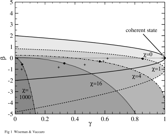
FIG. 1.: Representation of physically-realizable ensembles, arising from general continuous Markovian unravelings (CMU), for $\nu=0$ and various values of $\chi$. The shaded regions represent values of $\gamma$ and $\beta$ (and thus $\alpha=(1+\beta^{2})/\gamma$) that can be realized by monitoring. The progressively-darker shaded regions correspond to values of $\chi$ of 0, 1, 4, 16 and 1000 and are bounded by solid, dashed, dash-doted, dotted and dash-dot-doted curves, respectively. The $\gamma$, $\beta$ value of the closest-to-coherent (CC) ensemble in each region is marked as a filled circle on the boundary. The crosses mark the $\gamma$, $\beta$ values of the quantum-state diffusion (QSD) ensembles for the same set of $\chi$ and $\nu$ values, with the $\chi$ values reducing from left to right.

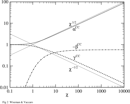
FIG. 2.: The parameters for the physically-realizable ensemble that is closest to a coherent ensemble (CC) as a function of $\chi$ with $\nu=0$. The ensembles arise from general continuous Markovian unravelings. These parameters are the phase quadrature variance $\alpha^{\rm CC}$ (dotted line), the amplitude-quadrature variance $\gamma^{\rm CC}$ (dashed line) and the covariance $\beta^{\rm CC}$ (dash-dot line) for the members of this ensemble. Also shown for comparison are thin solid curves representing $\chi^{1/2}$ and $\chi^{-1/2}$.

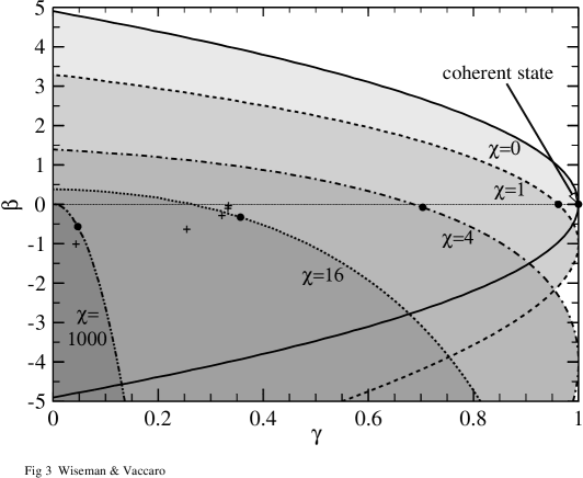
FIG. 3.: Representation of physically-realizable ensembles similar to Fig. 1 but for $\nu=10$.

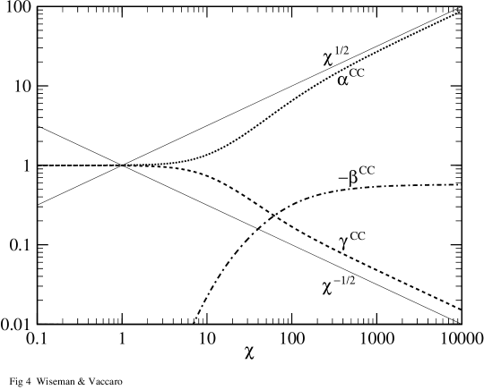
FIG. 4.: The parameters for the closest-to-coherent physically realizable (CC PR) ensemble as a function of $\chi$ similar to Fig. 2 but here with $\nu=100$. The excess phase diffusion allows the realization of states very close to coherent states until $\chi\sim\nu^{1/2}$

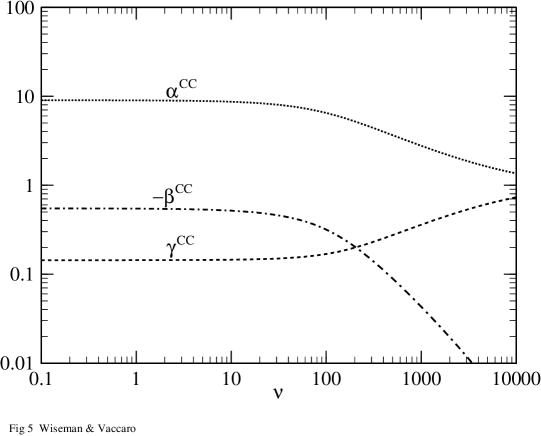
FIG. 5.: The parameters of the closest-to-coherent physically-realizable (CC PR) ensemble similar to Fig. 2 but here as a function of $\nu$ and with $\chi=100$.

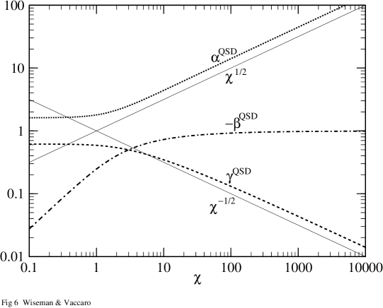
FIG. 6.: The parameters of the ensemble arising from quantum state diffusion (QSD) as a function of $\chi$ with $\nu=0$. The labeling follows Fig. 2.

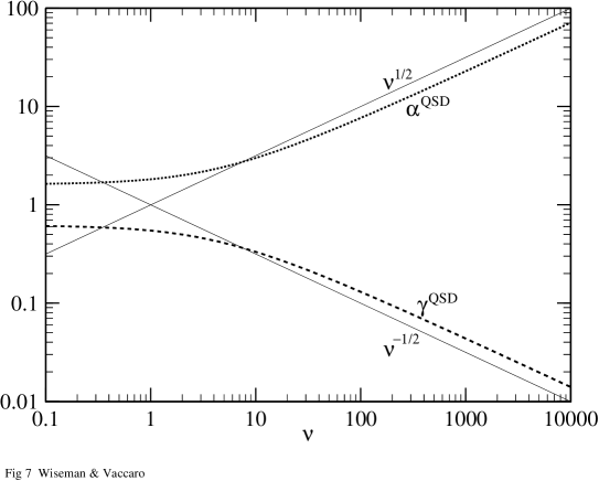
FIG. 7.: Similar to Fig. 6 but as a function of $\nu$ with $\chi=0$. The thin solid curves represent values of $\nu^{1/2}$ and $\nu^{-1/2}$.

- [1] K. Mølmer, Phys. Rev. A 55, 3195 (1996).
- [2] J. Gea-Banacloche, Phys. Rev. A 58, 4244 (1998); K. Mølmer, ibid., 4247 (1998).
- [3] H.M. Wiseman, Phys. Rev. A 56, 2068 (1997).
- [4] M. Sargent, M.O. Scully, and W.E. Lamb, Laser Physics (Addison-Wesley, Reading Mass., 1974)
- [5] W.H. Louisell, Quantum Statistical Properties of Radiation (John Wiley & Sons, New York, 1973).
- [6] H.M. Wiseman and J.A. Vaccaro, part II, to be published in Phys. Rev. A., quant-ph/0112145
- [7] H.M. Wiseman and J.A. Vaccaro, Phys. Lett. A 250, 241 (1998).
- [8] H.J. Carmichael, An Open Systems Approach to Quantum Optics (Springer-Verlag, Berlin, 1993).
- [9] H.M. Wiseman, Phys. Rev. A 60, 4083 (1999).
- [10] H.M. Wiseman and M.J. Collett, Phys. Lett. A 202, 246 (1995).
- [11] R.J.C. Spreeuw, T. Pfau, U. Janicke, and M. Wilkens, Europhys. Lett. 32, 469 (1995).
- [12] M. Olshanii, Y. Castin, and J. Dalibard, in Proc. XII Conference on Lasers Spectroscopy, edited by M. Inguscio, M. Allegrini and A. Sasso (World Scientific, 1995).
- [13] M. Holland et al, Phys. Rev. A 54, R1757 (1996).
- [14] M.H. Anderson et al, Science 269, 198 (1995).
- [15] C.C Bradley, C.A. Sackett, J.J. Tollett, and R.G. Hulet, Phys. Rev. Lett. 75, 1687 (1995).
- [16] K.B. Davis et al., Phys. Rev. Lett. 75, 3969 (1995).
- [17] M.-O. Mewes, M. R. Andrews, D. M. Kurn, D. S. Durfee, C. G. Townsend, and W. Ketterle, Phys. Rev. Lett. 78, 582 (1997)
- [18] B.P. Anderson, M.A.Kasevich, Science 282, 1686 (1998).
- [19] E.W. Hagley, L. Deng, M, Kozuma, J. Wen, K. Helmerson, S.L. Rolston, W.D. Phillips, Science 283, 1706 (1999);
- [20] I. Bloch, T.W. Hänsch, and T. Esslinger Phys. Rev. Lett. 82, 3008 (1999).
- [21] C.W. Gardiner, Quantum Noise (Springer, Berlin, 1991).
- [22] G. Lindblad, Commun. math. Phys. 48, 199 (1976).
- [23] J. von Neumann, Mathematical Foundations of Quantum Mechanics (Springer, Berlin, 1932); English translation (Princeton University Press, Princeton, 1955).
- [24] J. Dalibard, Y. Castin and K. Mølmer, Phys. Rev. Lett. 68, 580 (1992).
- [25] C.W. Gardiner, A.S. Parkins, and P. Zoller, Phys. Rev. A 46, 4363 (1992).
- [26] H.M. Wiseman and G.J. Milburn, Phys. Rev. A 47, 1652 (1993).
- [27] J.A. Vaccaro and D. Richards, Phys. Rev. A 58, 2690 (1998).
- [28] V.P. Belavkin, “Nondemolition measurement and nonlinear filtering of quantum stochastic processes”, pp. 245-66 of A. Blaquière (ed.), Lecture Notes in Control and Information Sciences 121 (Springer, Berlin, 1988).
- [29] V.P. Belavkin and P. Staszewski, Phys. Rev. A 45, 1347 (1992).
- [30] A. Barchielli, Quantum Opt. 2, 423 (1990).
- [31] A. Barchielli, Int. J. Theor. Phys. 32, 2221 (1993).
- [32] H.M. Wiseman and G.J. Milburn, Phys. Rev. A 47, 642 (1993).
- [33] H.M. Wiseman and L. Diósi, to be published in J. Chem. Phys. (2001). [quant-ph/0012016]
- [34] Quant. Semiclass. Opt. 8 (1) (1996), special issue on “Stochastic quantum optics”, edited by H.J. Carmichael.
- [35] M. Rigo and N. Gisin, p. 255 of Ref. [34] (1996).
- [36] H.M. Wiseman and G.E. Toombes, Phys. Rev. A 60, 2474 (1999).
- [37] H.M. Wiseman, p. 205 of Ref. [34] (1996).
- [38] C.W. Gardiner, Handbook of Stochastic Methods (Springer, Berlin, 1985).
- [39] L. Diósi, Phys. Lett. A 132, 233 (1988).
- [40] N. Gisin and I. Percival, Phys. Lett. A 167, 315 (1992); ibid., J. Phys. A 25, 5677 (1992).
- [41] L. Diósi and C. Kiefer, Phys. Rev. Lett. 85, 3552 (2000).
- [42] R. Dum, P. Zoller and H. Ritsch, Phys. Rev. A 45, 4879 (1992).
- [43] H.M. Wiseman, Phys. Rev. A 47, 5180 (1993).
- [44] H.M. Wiseman and J.A. Vaccaro, Phys. Rev. Lett. 87, 240402 (2001)
- [45] L.P. Hughston, R. Jozsa, and W.K. Wootters, Phys. Lett. A 183, 14 (1993).
- [46] G.J. Milburn and C.A. Holmes, Phys. Rev. Lett. 56, 2237 (1986).
- [47] H.M. Wiseman and L.K. Thomsen, Phys. Rev. Lett. 86, 1143 (2001).
- [48] G. Baym and C.J. Pethick, Phys. Rev. Lett. 76, 6 (1996).
- [49] S. Stringari, Phys. Rev. Lett. 77, 2360 (1996).
- [50] J. Ruostekoski, T. Gasenzer and D.A.W. Hutchinson, Mater-wave coherence of an atom laser with pulsed Raman output coupler (unpublished).