Continuous Quantum Measurement and the Emergence of Classical Chaos LA-UR-99-3187

Abstract

We formulate the conditions under which the dynamics of a continuously measured quantum system becomes indistinguishable from that of the corresponding classical system. In particular, we demonstrate that even in a classically chaotic system the quantum state vector conditioned by the measurement remains localized and, under these conditions, follows a trajectory characterized by the classical Lyapunov exponent.

The emergence of classical chaos from quantum mechanics is probably the most important theoretical problem in the study of the quantum to classical transition. Because of the absence of chaos in isolated quantum systems noqc and the noncommutativity of the twin limits $\hbar\rightarrow 0$ (the semiclassical limit) and $t\rightarrow\infty$ (the late-time limit, necessary to describe chaos), the fundamental mechanism of how classical chaos arises from quantum mechanics remains to be elucidated. While there has been much progress recently in the development of sophisticated semiclassical methods for chaotic dynamical systems semiclass , attempts to unambiguously characterize notions of chaos in the exact quantum dynamics attempts and to extract classical chaos as a formal semiclassical limit have been less successful: a rigorous quantifier of ‘quantum chaos’ on par with the classical Lyapunov exponents has yet to be found. And, since formal techniques have so far not succeeded in extracting trajectories from isolated quantum systems, they have not been able to explain the generation of chaotic time series in actual experimental situations. The experimental state of the art has, however, reached the stage where the quantum to classical transition can now be probed directly expts . So, it is crucial that one understand the mechanism underlying this transition in order to interpret existing results and design future experiments.

As real experiments always deal with open systems, and the interaction with the measuring apparatus necessary to deduce classical behavior provides an irreducible disturbance on the free evolution of the quantum system, the resulting decoherence and conditioned evolution could play a crucial role in the emergence of the classical limit, and of chaos, from the underlying quantum dynamics. Indeed, some qualitative results in this direction already exist hzs ; qsd . In this Letter, we show that, even in the absence of any other interaction with the environment, the theory of continuous quantum measurements applied to the quantum dynamics of classically chaotic systems provides a quantitatively satisfactory explanation of how classical chaos, and Lyapunov exponents characterizing it, emerges from quantum mechanics.

Open quantum systems are often studied by writing the evolution equation for the reduced density matrix obtained by tracing over the degrees of freedom in the environment. Although this process, called decoherence, can be extremely effective in suppressing interference effects and thereby making the quantum Wigner function approach the corresponding classical phase space distribution function hzs , it does not succeed in extracting localized ‘trajectories’ from the quantum dynamics. Without the existence of such trajectories it is extremely difficult, if not impossible, to rigorously quantify the existence of chaos both mathematically and in actual experimental practice. Since in order to extract classical trajectories systems must be observed, one expects observed quantum systems to obey classical dynamics in the macroscopic limit.

What is therefore desired is an unraveling of the Master equation which provides a more detailed understanding of the trajectories underlying the average system dynamics. When these detailed trajectories follow classical dynamics (albeit noisy), one can infer that the average distributions generated by them also become classical. This then provides a ‘microscopic’ understanding of the quantum to classical transition demonstrated, e.g., in Ref. hzs .

The first requirement in this program is to have a good model of continuous quantum measurement. Even though ‘continuous’ measurement is always an idealization, real experimental situations exist which approximate it extremely closely, and simple models which correspond accurately to these processes have now been developed cqm1 ; cqm1a ; cqm2 ; cqm3 . These models show that as a necessary result of the information it provides, continuous measurement produces and maintains localization in phase space. On the other hand, the Ehrenfest theorem guarantees that well-localized quantum systems effectively obey classical mechanics. As the measurement process, in addition to localizing the state, also introduces a noise in its evolution, to obtain classical mechanics one must be in a regime in which the localization is sufficiently strong and, yet, the resulting noise sufficiently weak. We show that such a regime exists, and is precisely the one which governs macroscopic objects, i.e. $\hbar\ll S$, the action of the system. In what follows, we refer to this regime as the classical regime. Our central result is that, once this regime is achieved, the localized trajectories for the continuously observed quantum system obey the classical dynamics (possibly chaotic) for that system driven by a weak noise. As a result, even at a finite but non-zero value of $\hbar$, the quantum ‘trajectories’ possess the same Lyapunov exponents as the corresponding classical system. As one goes deeper into the classical regime with $\hbar\rightarrow 0$, one can make the noise progressively smaller by optimizing the measurement, and, in the limit, the intrinsic classical Lyapunov exponents are recovered.

In order for this mechanism to satisfactorily explain the quantum-classical transition, the following conditions need to be satisfied: (1) localization as discussed above, (2) suppression of measurement noise, (3) the actual value of the measurement strength should become irrelevant, and (4) the measurement record (i.e., the actual results of the continuous measurement process), suitably band-limited, should follow the classical trajectory. These conditions are studied in more detail below.

We consider, for simplicity, a single quantum degree of freedom, with position and momentum operators denoted by $X$ and $P$, evolving under an unperturbed Hamiltonian $P^{2}/2m+V(X)$. Quantum mechanics then dictates the familiar Heisenberg equations of motion for these operators: $\dot{X}=P/m$, and $\dot{P}=-\partial_{X}V(X)\equiv F(X)$. Except in the limit $\hbar\to 0$, a continuous observation with finite measurement strength does not localize either the position or the momentum completely. Nevertheless, we can describe the state of the particle in terms of the central moments of $X$ and $P$ and, anticipating the limit, assign it to a point in phase space given by the mean values $\langle X\rangle$ and $\langle P\rangle$.

The most natural measurement to use is a continuous measurement of position, not only because this is often what is observed with mechanical detectors, but also because real schemes for the continuous measurement of position, considered in the field of quantum optics, may be described very simply measx . In addition, a continuous measurement of position is an unraveling of the thermal Master equation in the high temperature limit, so that results demonstrated for this case also apply to decoherence due to a weakly coupled, high temperature thermal bath. We stress however, that we do not expect the particular measurement model to effect the results significantly; any measurement or interaction which produces a localization in phase space should lead to classical behavior in essentially the same manner.

Under continuous position measurement the evolution of the wavefunction becomes stochastic. The stochastic master equation for the density matrix $\rho(t)$, conditioned on the measurement record $\langle X\rangle+\xi(t)$ with $\xi(t)\equiv(8\eta k)^{-1/2}dW/dt$, is measx

$$\rho(t+dt) = \rho-(\frac{i}{\hbar}[H,\rho]-k[X,[X,\rho]])\mathbin{}dt$$ (1)

$${}+\sqrt{2\eta k}\mathbin{}([X,\rho]_{+}-2\rho\mathop{\rm Tr}\rho X)\mathbin{}dW\,,$$

where $k$ is a constant specifying the strength of the measurement, $\eta$ is the measurement efficiency and is a number between 0 and 1, and $dW$ is a Weiner process, satisfying $(dW)^{2}=dt$. When $\eta=1$, the evolution preserves the purity of the state and can be rewritten in a way which allows it to be understood as a series of diffuse projection measurements cqm2 on an unnormalized wavefunction $\tilde{\psi}$:

$$|\tilde{\psi}(t+dt)\rangle=e^{-2kdt(X-(\langle X\rangle+\xi(t)))^{2}}e^{-iHdt/\hbar}|\tilde{\psi}(t)\rangle,$$ (2)

where $\xi(t)$, the difference between $\langle X\rangle$ and the measured value of the position, becomes a white noise in the limit that $dt$ tends to zero. Under this continuous measurement process, the average values of position and momentum evolve according to

$$d\langle X\rangle = (\langle P\rangle/m)dt+\sqrt{2k}V_{x}(t)dW$$ (3)

$$d\langle P\rangle = \langle F(X)\rangle dt+\sqrt{2k}C_{xp}(t)dW,$$ (4)

where $V_{x}$ is the variance in position, and $C_{xp}$ is the symmetrized covariance between $X$ and $P$ eomav . Thus the effect of the measurement is to provide some zero-mean noise proportional to the square root of the measurement strength $k$ and to the width of the distribution. It is important to note, however, that this is just the first in a hierarchy of equations for the moments; the equations governing the second moments contain terms depending on higher moments, and so on up the hierarchy.

Even though the structure of the hierarchy makes it almost impossible to obtain analytic answers to questions regarding the behavior of the variances, and resulting noise strength, which are the crucial quantities determining the quantum to classical transition, we can, nevertheless discuss the effect of varying $\hbar$ by truncating the hierarchy at the second order, and looking at the steady state solution for the variances. These equations show that to maintain enough localization to guarantee that, at a typical point on the trajectory, $\langle F(x)\rangle\approx F(\langle x\rangle)$, as required in the classical limit, the measurement strength, $k$, must stop the spread of the wavefunction at the unstable pointsfootnote1 , $\partial_{x}F>0$:

$$8\eta k\gg\frac{\partial_{x}^{2}F}{F}\sqrt{\frac{\partial_{x}F}{2m}}\,.$$ (5)

Note that this condition is automatically satisfied for linear systems, where quantum dynamics of the expectation values are identical with classical evolution.

On the other hand, a large measurement strength introduces noise into the trajectory. If we demand that averaged over a characteristic time period of the system, the change in position and momentum due to the noise are small compared to those induced by the classical dynamics, it is sufficient that, at a typical point on the trajectory, the measurement satisfy

$$\frac{2\left|\partial_{x}F\right|}{\eta s}\ll\hbar k\ll\frac{\left|\partial_{x}F\right|s}{4}\,,$$ (6)

where $s$ is the typical value of the actionfootnote2 of the system in units of $\hbar$. Obviously as $s$ becomes much larger than $2\sqrt{2}\eta^{-1/2}$, this relationship is satisfied for an ever larger range of $k$, and this defines the classical limit.

Finally, in experiments one usually considers the measurement record itself rather than the estimated state of the system as we have done. As measurement introduces a white noise, it is important to investigate the condition under which the record tracks the estimate faithfully. If $\Delta t$ is the time over which the continuous measurement is averaged to obtain the record, and we allow ourselves a maximum of $\Delta x$ as the position noise, it is easy to see that the measurement strength needs to satisfy

$$8\eta k>\frac{1}{\Delta t(\Delta x)^{2}}$$ (7)

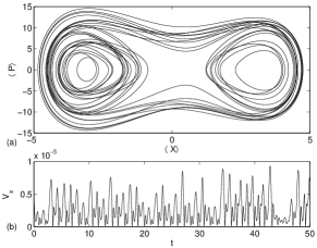
Figure 1: (a) The quantum trajectory in phase space, with $\hbar=10^{-5}$ and $k=10^{5}$. (b) The position variance, $V_{x}$, as a function of time.

With this introduction, we consider, as an example, a bounded, one-dimensional, driven system with the Hamiltonian,

$$H=P^{2}/2m+BX^{4}-AX^{2}+\Lambda X\cos(\omega t)~{}.$$ (8)

with $m=1$, $B=0.5$, $A=10$, $\Lambda=10$, $\omega=6.07$. This Hamiltonian has been used before in studies of quantum chaos linbal and quantum decoherence hzs and, in the parameter regime used here, a substantial area of the accessible phase space is stochastic. The numerical method used to solve Eq. (1) is a split-operator, spectral algorithm implemented on a parallel supercomputer.

Simulations at various values of $\hbar$ confirm that as $\hbar$ is reduced, both the steady-state variance, and the resulting noise (for optimal measurement strengths) are reduced, as expected. As the dynamical time scale of this problem is $1-0.1$, we decide to average the continuous observation record over a period of $0.01$. Similarly, as the range of the motion covers distances of $O(10)$, we demand that the position be tracked to an accuracy of $0.01$. By Eq. 7, this means we need $\eta k\sim O(10^{5})$ or larger. In our example, we choose the energy to be $O(10^{2})$, and the corresponding typical action turns out to be $O(10)$, and the typical nonlinearity makes the rhs of Eq. 5 $O(1)$. We see that a choice of $\hbar=10^{-5}$, $\eta=1$ and $k=10^{5}$, satisfies all the constraints for a classical motion. In Fig. 1 we demonstrate that in this regime, localization is maintained in spite of low noise. Fig. 1(a) shows a typical phase space trajectory, with the position variance during the evolution, $V_{x}\equiv(\Delta X)^{2}$, plotted in Fig. 1(b). We find that the width $\Delta X$ is always bounded by $3.4\times 10^{-3}$. Furthermore, as is immediately evident from the smoothness of the trajectory in Fig. 1(a), the noise is also negligible on these scales.

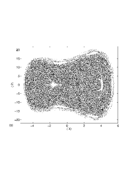
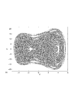
Figure 2: (a) The quantum stroboscopic map with $\hbar=10^{-5}$ and $k=10^{5}$. The figure is a pastiche from several different runs with different initial conditions, for a total duration of $39,000$ periods of the temporal drive. (b) The stroboscopic map for the corresponding classical system, driven with a small amount of noise.

Thus, we find that continuous measurement can effectively obtain classical mechanics from quantum mechanics. We substantiate this further by demonstrating that the trajectories we obtain show the common signatures of classical chaos. A direct way to compare qualitatively the global nature of the quantum and classical trajectories in phase space is to compare the stroboscopic maps (the distribution of the locations of the system at a constant phase of the driving term). Fig. 2 demonstrates the excellent correspondence between the classical and quantum maps in this regard.

On a more quantitative level, we now calculate the key characteristic of chaos, the maximal Lyapunov exponent, $\lambda$, and compare it against that of the classical system driven with a similar amount of noise. We start with the definition of $\lambda$: that for a chaotic system the distance between two nearby trajectories, $\Delta(t)$, evolves, on average, as $\ln\Delta(t)\sim\lambda t$, as long as $\Delta(t)$ is small and $t$ is large. To calculate this we take 10 fiducial trajectories (9 in the quantum case) starting at the point (-3,8) and at 17 points along each trajectory, separated by time intervals of 20 each, we obtain neighboring trajectories by varying the noise realization. The distance between the fiducial and these neighboring trajectories is tracked for a time interval of 8. The values of $\ln\Delta(t)$ thus obtained are averaged over all the instances and plotted versus $t$ in Fig. 3, both for the classical (with a small amount of noise) and the continuously measured quantum systems. For very small separations $\Delta$, the noise dominates, which gives rise to an initial steep slope. This is followed by a linear region dominated by the Lyapunov exponent. Eventually $\Delta(t)$ becomes large and the curve flattens out. The behavior of the observed quantum and noisy classical systems are essentially indistinguishable, and the Lyapunov exponent $0.57(2)$ is the same for both. Performing the analysis with the classical system without noise, this time using 50 fiducial trajectories with initial points in a neighborhood of (-3,8), we obtain a Lyapunov exponent of $0.56(1)$, in agreement with the previous values.

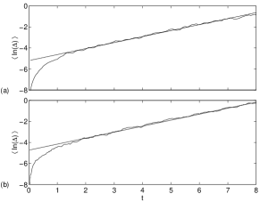
Figure 3: Lyapunov exponents, $\lambda$, calculated for (a) the classical system driven with a small amount of noise, and (b) the continuously observed quantum system, with $\hbar=10^{-5}$ and $k=10^{5}$. The slope of the line drawn through the curves gives the Lyapunov exponent, which in both cases is $\lambda=0.57(2)$.

After having demonstrated that in the classical regime, the localization and low noise conditions are satisfied simultaneously, we study the sensitivity to the measurement strength. To this effect, we vary $k$ between $2\times 10^{4}$ and $5\times 10^{5}$. The Lyapunov exponents remained unchanged within the quoted errors; only at $k=5\times 10^{5}$ did the noise start to wash out the flat region of the curve.

References

- (1) H.J. Korsch and M.V. Berry, Physica D 3, 627 (1981); T. Hogg and B.A. Huberman, Phys. Rev. Lett. 48, 711 (1982); R.L. Ingram, M.E. Goggin and P. W. Milonni, in Coherence and Quantum Optics VI, edited by J.H. Eberly (Plenum, New York, 1990).
- (2) M.C. Gutzwiller, J. Math. Phys. 12, 343 (1971); See also E.J. Heller and S. Tomsovic, Phys. Today 46, 38 (1993).
- (3) See, e.g., A. Peres, Phys. Rev. A 30, 1610 (1984); M. Toda and K. Ikeda, Phys. Lett. A 124, 165 (1987); Y. Gu, ibid 149, 95 (1990); R. Schack and C.M. Caves, Phys Rev. E. 53, 3257 (1996), Eprint: quant-ph/9506008.
- (4) M. Brune, E. Hagley, J. Dreyer, X. Maitre, A. Maali, C. Wunderlich, J. M. Raimond, and S. Haroche, Phys. Rev. Lett. 77, 4887 (1996); C.J. Hood, M.S. Chapman, T.W. Lynn, and H.J. Kimble, ibid 80, 4157 (1998); H. Ammann, R. Gray, I. Shvarchuck, and N. Christensen, ibid 80, 4111 (1998); B.G. Klappauf, W.H. Oskay, D.A. Steck, and M.G. Raizen, ibid 81, 1203 (1998).
- (5) S. Habib, K. Shizume, and W.H. Zurek, Phys. Rev. Lett. 80, 4361 (1998), Eprint: quant-ph/9803042.
- (6) T.P. Spiller and J.F. Ralph, Phys. Lett. A 194, 235 (1994); T.A. Brun, I.C. Percival, and R. Schack, J. Phys. A 29, 2077 (1996), Eprint: quant-ph/9509015.
- (7) Early work includes A. Barchielli, L. Lanz and G.M. Prosperi, Nuovo Cimento 72B, 79 (1982); N. Gisin, Phys. Rev. Lett. 52, 1657 (1984); L. Diosi, Phys. Lett. A 114, 451 (1986); for a review see, A. Barchielli, Int. J. Theor. Phys. 32, 2221 (1993).
- (8) V.P. Belavkin and P. Staszewski, Phys. Lett. A 40, 359 (1989).
- (9) C.M. Caves and G.J. Milburn, Phys. Rev. A. 36, 5543 (1987).
- (10) H. Carmichael, An Open Systems Approach to Quantum Optics (Springer-Verlag, Berlin, 1993); H.M. Wiseman and G.J. Milburn, Phys. Rev. A 47, 642 (1993).
- (11) A.C. Doherty and K. Jacobs, Phys. Rev. A 60, 2700 (1999), Eprint: quant-ph/9812004.
- (12) J.K. Breslin and G.J. Milburn, Phys. Rev. A 55, 1430 (1997); J. Halliwell and A. Zoupas, Phys. Rev. D 52, 7294 (1995), Eprint: quant-ph/9503008.
- (13) Actually, if the nonlinearity is large on the quantum scale, , needs to be much larger than , irrespective of the sign of . This does not change the argument in the body of the paper.
- (14) We are assuming that both and evaluated at a typical point of the trajectory are comparable to the action of the system, and define this to be .
- (15) W.A. Lin and L.E. Ballentine, Phys. Rev. Lett. 65, 2927 (1990).