Classical behaviour of many-body systems in Bohmian Quantum Mechanics

Abstract

The classical behaviour of a macroscopic system consisting of a large number of microscopic systems is derived in the framework of the Bohmian interpretation of quantum mechanics. Under appropriate assumptions concerning the localization and factorization of the wavefunction it is shown explicitly that the center of mass motion of the system is determined by the classical equations of motion.

, and

1 Introduction

A deterministic formulation of quantum mechanics, which is equivalent to the usual theory with respect to the prediction of experimental results, had originally been proposed by D. Bohm [1] and attracted some interest recently [2, 3, 4, 5, 6]. This alternative interpretation provides additional insight in various topics in quantum mechanics like the definition of quantum chaos analogously to the classical case [7, 8, 9] or the derivation of the statistical postulates of a measurement process from a deterministic theory [10].

Due to the nature of the theory containing a classical particle, whose dynamics is determined by the quantum mechanical wavefunction, the transition from quantum behaviour for elementary particles and classical motion of heavy point particles is continous. In this framework the classical limit is simpler and more intuitive than in the conventional theory, avoiding e.g. the introduction of coherent states [3, 6, 11].

The problem, why normal macroscopic objects, which are not elementary, but contain a large number of microscopic, quantum mechanical subsystems, behave classically, is much less trivial and has up to now not been worked out in the framework of the Bohmian theory. An additional important issue is to understand the relation between the nonpredictibility features of the quantum mechanical measurement process [3, 5, 6, 11] and a classical measurement, which does not affect the state of the system. The proof that the center of mass motion of a macroscopic system is under certain assumptions classical will be the main aim of the following investigations. The necessary characterizations of the wavefunction will thereby have a simple intuitive meaning in terms of forces on the Bohmian particle.

The paper is organized as follows: After a short review of the Bohmian formulation of quantum mechanics (chap. 2), the classical limit of macrocopic objects is characterized (chap. 3) and the classical equations of motion for the center of mass coordinates are derived (chap. 4).

2 Bohmian quantum mechanics

Within the Bohmian mechanics [2, 1, 3, 4, 5, 6], a state of a system is completely determined not only by the wavefunction $\Psi$, but also by the position $x(t)=(x_{1},\ldots,x_{N})(t)$ of a hidden particle in the configuration space of the system.

The dynamics of the wavefunction $\Psi$ is determined by the Schrödinger equation in the usual way, while the dynamics of the particle is deduced from the wavefunction $\Psi(x,t)$.

By introducing the modulus $R(x,t)$ and the phase $S(x,t)$ of the wavefunction $\Psi(x,t)=R(x,t)e^{\frac{i}{\hbar}S(x,t)}$ the Schrödinger equation can be written as

$$-\frac{\partial}{\partial t}S(x,t)=\frac{(\frac{\partial}{\partial x}S(x,t))^{2}}{2m}-\frac{\hbar^{2}}{2m}\frac{\frac{\partial^{2}}{\partial x^{2}}R(x,t)}{R(x,t)}+V(x,t),$$ (1)

$$\frac{\partial}{\partial t}R(x,t)^{2}+\frac{\partial}{\partial x}\Big{(}R(x,t)^{2}\frac{\frac{\partial}{\partial x}S(x,t)}{m}\Big{)}=0.$$ (2)

While equation (2) represents a continuity equation of $|\Psi(x,t)|^{2}$, equation (1) is a Hamilton Jacobi equation of a classical particle with coordinate $x$ in the presence of both the classical potential $V(x,t)$ and the so-called quantum potential [1]

$$Q(x,t):=-\frac{\hbar^{2}}{2m}\frac{\frac{\partial^{2}}{\partial x^{2}}R(x,t)}{R(x,t)}\quad.$$ (3)

In particular the momentum $p(t)$ and the energy $E(t)$ of the particle are given by derivatives of the phase $S(x,t)$ of the wavefunction $\Psi(x,t)$:

$$p(t):=m{\dot{x}}=\frac{\partial}{\partial x}S(x,t)|_{x(t)}\quad,\quad E(t):=-\frac{\partial}{\partial t}S(x,t)|_{x(t)}\quad.$$ (4)

This first-order differential equation is sufficient to calculate the trajectory $x(t)$ from the initial value $x(t_{0})$, but the relative significance of classical and quantum mechanical effects becomes clearer in a different representation. After a straightforward calculation (cf. appendix A) the equation of motion of the Bohmian particle $x(t)$ can be presented in a form, which is similar to Newton’s law, but contains a quantum force $F_{Q}:=-\frac{\partial}{\partial x}Q$ in addition:

$$\frac{d}{dt}p(t)=-\frac{\partial}{\partial x}\Big{(}V(x,t)+Q(x,t)\Big{)}\Big{|}_{x(t)}=:F(t)\quad.$$ (5)

3 Characterisation of classical many-body systems

One of the intuitive features of the Bohmian formulation of quantum mechanics is the fact that there is a continous and simple limit from the quantum to the classical regime of a single degree of freedom. By increasing the mass $m$ of the particle, i.e. $\frac{\hbar^{2}}{2m}\rightarrow 0$, the quantum force $F_{Q}=-\partial_{x}Q\rightarrow 0$ in equ. 5 vanishes and the quantum potential $Q={\rm const.}$ becomes irrelevant in the Hamilton-Jacobi equation 1. The absence of quantum mechanical interactions $\sim Q$ in addition to the classical potential $V(x)$ also provides a natural explanation, why the state of a classical system of this kind will not be affected during a measurement.

If and under what circumstances the collective motion of objects consisting out of a macrocopic number $N\sim 10^{23}$ of quantum mechanical systems of mass $m$ with $\frac{\hbar^{2}}{2m}\sim O(1)$ is classical, is far less obvious and will be investigated in the following. Thereby it turns out that additional assumptions have to be made in order to recover classical physics and to exclude macroscopic quantum phenomena like superconductivity or superfluidity.

Let the macrocopic system consist of $N$ subsystems, e.g. atoms, with center of mass coordinates $x_{i}(t)$ for $i\in\{1,\ldots,N\}$, which are determined by the wavefunction

$$\Psi_{\rm sym}(x_{1},\ldots,x_{N},t) = \sum_{\nu=1}^{N!}c_{\nu}\Psi(x_{\pi_{\nu}(1)},\ldots,x_{\pi_{\nu}(N)},t)=$$ (6)

$$=: \sum_{\nu=1}^{N!}c_{\nu}\Psi_{\nu}(x_{1},\ldots,x_{N},t)\quad.$$ (7)

Thereby the exchange symmetry of the indistinguishable particles has been built in by a summation over the permutations $\pi_{\nu}$ ($\nu=1,\dots,N!$) with appropriate coefficients $c_{\nu}$.

Having in mind classical systems like solids, fluids or gases consisting of a large number of atoms, which show no quantum behaviour like Bose-Einstein condensation, we can assume the following two features:

(i) Locality: The quantum mechanical motion of the center of mass coordinates of different subsystems, which are determined by the wavefunction $|\Psi|^{2}$ via equ. 1, are assumed to be confined to disjunct regions in configuration space. This can be motivated by the physical picture that the quantum mechanical uncertainity of the position of the center of mass is much smaller than the minimal distance, i.e. the radius of the atom, of the subsystems.

More explicitly this feature manifests itself as a vanishing overlap of the functions $\Psi_{\nu}$ corresponding to different permutations of the center of mass coordinates:

$$\int\!\!dx_{1}\cdots dx_{N}\,\Psi^{*}(x_{\pi_{\nu}(1)},\ldots x_{\pi_{\nu}(N)},t)\Psi(x_{\pi_{\tilde{\nu}}(1)},\ldots x_{\pi_{\tilde{\nu}}(N)},t)=\delta_{\nu{\tilde{\nu}}}\;.$$ (8)

In the Bohmian interpretation this means that the particle $(x_{1},\dots,x_{N})(t)$ cannot tunnel from the support $\Gamma_{\nu}:=\{x\in\Rset^{N}|\Psi_{\nu}(x)=\partial_{i}\Psi_{\nu}(x)=0\quad\forall i\}$ of one wavepacket $\Psi_{\nu}$ to another. Consequently the ergodicity of its trajectory $x(t)$ is restricted to a certain subset $\Gamma_{\mu}$ and the other parts $\Psi_{\nu}$ ($\nu\neq\mu$) of the wavefunction can be neglected without loss of generality. Note that here the selection of a certain sector $\mu$ is given by the position of the particle and not due to the collapse of the wavefunction after a measurement.

As an example the expectation value

$$\bar{x}_{i}(t):=\int\!\!dx_{1}\cdots\int\!\!dx_{N}\,\Psi^{*}_{\mu}(x_{1},\dots,x_{N},t)x_{i}\Psi_{\mu}(x_{1},\ldots,x_{N},t)$$ (9)

of the center of mass coordinate $x_{i}$ has to be averaged over the support $\Gamma_{\mu}$ only. Note that $\bar{x}_{i}(t)$ denotes the average position of the center of mass in an infinite number of measurements and is not identical with the position $x_{i}(t)$ of the Bohmian particle. The locality assumption (i) can therefore be expressed more precisely by the statement that $|x_{i}(t)-\bar{x}_{i}(t)|$ is small compared with the minimal distance of the center of mass coordinates of the subsystems. The wavefunction $\Psi_{\rm sym}(x_{1},x_{2},t)$ is expressed schematically for the two-dimensional case in figure 1 and the index $\mu$ of the wavefunction $\Psi_{\mu}$ will be suppressed in the following.

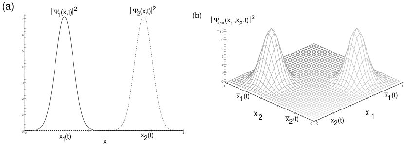
Figure 1: Schematic wavefunction of a system consisting of $N=2$ onedimensional subsystems: (a) The probability distributions $|\Psi_{i}(x,t)|^{2}$ ($i=1,2$) are localized around the values $\bar{x}_{i}$ and have vanishing overlap according to assumption (i) (cf. equ. 8). (b) The modulus $|\Psi_{\rm sym}(x_{1},x_{2},t)|=\frac{1}{\sqrt{2}}\Big{(}|\Psi_{1}(x_{1},t)|\,|\Psi_{2}(x_{2},t)|+|\Psi_{2}(x_{1},t)|\,|\Psi_{1}(x_{2},t)|\Big{)}$ of the total symmetrized wave function is localized around maxima at $(\bar{x}_{1},\bar{x}_{2})$ (i.e. $\nu=1$) and $(\bar{x}_{2},\bar{x}_{1})$ (i.e. $\nu=2$). Due to the vanishing overlap no transition of the system particle $(x_{1},x_{2})$ between the support $\Gamma_{\nu}$ of the two wavepackets $\nu=1,2$ is possible and it is sufficient to keep the part $\Gamma_{\mu}$, where the particle is located.

(ii) Factorization: In addition to this, the factorization of the wavefunction

$$\Psi(x_{1},\ldots,x_{N},t)=R_{1}(x_{1},t)\cdots R_{N}(x_{N},t)e^{\frac{i}{\hbar}S(x_{1},\ldots,x_{N},t)}$$ (10)

within each disjunct region $\Gamma_{\nu}$ turns out to be essential for the elimination of macroscopic quantum mechanical correlations. This assumption corresponds to the (ad hoc) introduction of ”decoherence” for the reconstruction of classical mechanics from the conventional quantum theory [5] and will be justified intuitively in the following.

As a consequence, the modulus

$$|\Psi(x_{1},\ldots,x_{N},t)|=|\Psi_{1}(x_{1},t)|\cdots|\Psi_{i}(x_{i},t)|\cdots|\Psi_{N}(x_{N},t)|$$ (11)

factorizes due to the decoherence assumption (ii) of equ. 10 and the quantum potential

$$Q(x_{1},\ldots,x_{N},t)=Q_{1}(x_{1},t)+\cdots+Q_{N}(x_{N},t)$$ (12)

is a sum of one particle potentials. This means that the motion

$$m_{i}\ddot{x}_{i}=-\frac{\partial}{\partial x_{i}}V(x_{1},\ldots,x_{N},t)\Big{|}_{x(t)}-\frac{\partial}{\partial x_{i}}Q_{i}(x_{i},t)\Big{|}_{x_{i}(t)}$$ (13)

of the center of mass of a subsystem is correlated to the other subsystems via the classical potential $V(x_{1},\dots,x_{N})$ only. Here the physical meaning of equ. 10 becomes transparent: Short-range quantum mechanical processes within the subsystem $i$ can affect its center of mass motion, but have no effect on the other subsystems.

Formula equ. 11 can be simplified by noting that the probability distributions $|\Psi^{l(i)}(x,t)|^{2}$ of the Bohmian particles $x_{i}$ around the mean value $\bar{x}_{i}$ are identical for equivalent subsystems of the same type $l(i)\in\{1,\dots,n\}$:

$$|\Psi(x_{1},\ldots,x_{N},t)|=\prod_{i=1}^{N}|\Psi^{l(i)}\big{(}x_{i}-\bar{x}_{i}(t),t\big{)}|\quad.$$ (14)

The condition $N\gg n$ that there is a macroscopic number of subsystems of each type is fulfilled for macroscopic objects like solids with a small number of inequivalent sites or gaseous mixtures of different particles and is at least approximately true for amorphous glass-like objects.

4 Center of mass motion

Figure 2: $N$ microscopic quantum mechanical systems with the center of mass coordinates $x_{i}(t)$ and masses $m_{i}$ ($i\in\{1,\ldots,N\}$) form a macroscopic object with center of mass $x_{\rm CM}(t)$ (at the point $\star$), his dynamics being governed by classical equations of motion.

The center of mass coordinate

$$x_{\rm CM}(t):=\frac{1}{M}\sum_{i=1}^{N}x_{i}(t)m_{i}$$ (15)

of a macroscopic object with mass $M$ is given by the average of the center of mass coordinates $x_{i}$ of the microscopic subsystems.

Although the trajectory $x_{\rm CM}(t)$ can be derived from equ. 4 alone, this is not convenient, as the phase $S(x_{1},\dots,x_{N},t)$ depends not only on $x_{\rm CM}$, but on all variables $x_{i}$ and must be calculated by a solution of the full Schrödinger equation.

Using equ. 5 for the quantum mechanical dynamics of $x_{i}(t)$ instead one obtains

$$\ddot{x}_{\rm CM}(t)M=-\sum_{i=1}^{N}\frac{\partial}{\partial x_{i}}V(x_{1},\dots,x_{N},t)\Big{|}_{x(t)}\!\!-\!\!\sum_{i=1}^{N}\frac{\partial}{\partial x_{i}}Q(x_{1},\dots,x_{N},t)\Big{|}_{x(t)}.$$ (16)

In the classical contribution

$$-\sum_{i=1}^{N}\frac{\partial}{\partial x_{i}}V(x_{1},\ldots,x_{N},t)\Big{|}_{x(t)}=\sum^{N}_{{i,j}\atop{i\neq j}}F_{ij}+\sum_{i=1}^{N}F_{i}^{ext}=:F^{\rm ext}$$ (17)

the internal forces $F_{ij}$ from subsystem $j$ on $i$ cancel due to Newton’s law $F_{ij}=-F_{ji}$ and only the total external force $F^{\rm ext}$ remains. Due to equ. 14 the quantum force for a homogeneous system ($n=1$) is given by

$$F_{Q}^{\rm CM}:=-\sum_{i=1}^{N}\frac{\partial}{\partial x_{i}}Q(x_{1},\dots,x_{N},t)\Big{|}_{x(t)}\!=-\sum_{i=1}^{N}\frac{\partial}{\partial x_{i}}Q\big{(}x_{i}-\bar{x}_{i}(t),t\big{)}|_{x_{i}(t)},$$ (18)

where

$$Q\big{(}x_{i}-\bar{x}_{i}(t),t\big{)}:=-\frac{\hbar^{2}}{2m}\frac{\frac{\partial^{2}}{\partial x_{i}^{2}}|\Psi\big{(}x_{i}-\bar{x}_{i}(t),t\big{)}|}{|\Psi\big{(}x_{i}-\bar{x}_{i}(t),t\big{)}|}\;\;.$$ (19)

For large $N\gg 1$ it is possible to replace the sum in equ. 18 by an integral. Thereby it is necessary to introduce the distribution function ${\mathcal{P}}(x_{i}-\bar{x}_{i}(t),t)$ of the position $x_{i}(t)$ of the system particle around the center of mass $\bar{x}_{i}$. This is given by the condition ${\mathcal{P}}(x_{i}-\bar{x}_{i}(t),t)=|\Psi\big{(}x_{i}-\bar{x}_{i}(t),t\big{)}|^{2}$ of so-called quantum equilibrium [12], which can be derived from the quasi-ergodic dynamics of the system particle during a sequence of measurements [5, 10]. This leads to

$$F_{Q}^{\rm CM} := -\frac{1}{N}\sum_{i=1}^{N}\frac{\partial}{\partial x_{i}}Q\big{(}x_{i}-\bar{x}_{i}(t),t\big{)}\Big{|}_{x_{i}(t)}\approx$$ (20)

$$\approx -\int_{-\infty}^{\infty}\!du\,|\Psi\big{(}u-\bar{x}_{i}(t),t\big{)}|^{2}\frac{\partial}{\partial u}Q\big{(}u-\bar{x}_{i}(t),t\big{)}=0\;,$$ (21)

which is shown to vanish in appendix B. Thereby the error can be estimated to be smaller than $\frac{|F_{Q_{\rm max}}|}{N}$, $F_{Q_{\rm max}}$ being the largest single quantum force. Hence the total quantum force

$$\Big{|}\sum_{i=1}^{N}\frac{\partial}{\partial x_{i}}Q(x_{1},\ldots,x_{N},t)\Big{|}_{x_{1}(t),\ldots,x_{N}(t)}\leq|F_{Qmax}|.$$ (22)

on the center of mass is of microscopic magnitude and can therefore not accelerate the macroscopic object of mass $M$ substantially. This proofs Newton’s Law

$$\ddot{x}_{\rm CM}(t)M=F^{ext}\quad$$ (23)

for the collective center of mass motion. This result is also true in the general case $n\neq 1$, as in the case $n\ll N$ the above argument can be used independently for each type $l(i)\in 1,\dots,n$ of subsystems.

An important corollary of the calculation presented here is that there is no quantum mechanical interaction between collective classical coordinates of two macroscopic objects, one representing a measurement device and the other one being the system to be measured. Therefore in a classical measurement the effect of the quantum potentials of the underlying microscopic subsystems neither causes any uncertainity in the measurement result nor affects the system to be measured beyond the classical interaction.

In order to clarify our characterisation of conventional classical systems further, we would like to discuss briefly the case of a Bose-Einstein condensate

$$\Psi(x_{1},\ldots,x_{N},t)=R(x_{1},\dots,x_{N},t)e^{\frac{i}{\hbar}\Big{(}S(x_{1},t)+\cdots+S(x_{N},t)\Big{)}}\sim e^{\frac{i}{\hbar}\sum\limits_{i=1}^{N}mvx_{i}}\!,$$ (24)

where coherence of the phases $S_{i}(x_{i},t)=S(x_{i},t)$ of the subsystems is essential. Here the motion of the center of mass coordinate can most easily determined from equ. 4 directly as

$$\dot{x}_{CM}(t)=v\Longrightarrow x_{CM}(t)=v(t-t_{0})+x_{CM}(t_{0})\quad.$$ (25)

Here the fundamental nature of a macroscopic quantum phenomen in contrast to conventional classical objects becomes evident: As the acceleration $\ddot{x}_{CM}=0$ vanishes, the total quantum force is of the same order as the classical one, while for the system obeying equ. 11 the effect of quantum forces averages out on a macroscopic level.

5 Summary and Conclusions

The reconstruction of classical dynamics for ordinary macroscopic objects containing subsystems, which behave quantum mechanically, has been reviewed from the viewpoint of Bohmian quantum mechanics. In this formulation the quantum mechanical effects are contained exclusively in an additional quantum force appearing in the classical equations of motion of the system particle. In the case of a point particle of macroscopic mass ($\hbar^{2}/2m\rightarrow 0$) the quantum potential becomes irrelevant, defining the classical limit in a conceptually clear way. In contrast to this, it was shown that additional restrictions on a many-body wavefunction have to be employed to recover Newton’s Law for the center of mass motion.

One main assumption concerned the fact that the wave function is sufficiently localized to prevent the Bohmian center of mass particle of an atom from leaving this subsystem. In addition to this, an appropriate factorization of the modulus $|\Psi|$ of the wavefunction is essential (cf. equ. 10) in order to eliminate quantum mechanical correlations between the different (quantum mechanical) subsystems. In this case quantum phenomena can be ruled out on macroscopic scales and the effect of quantum forces on collective macroscopic variables averages out. The Bohmian interpretation thereby provides further insight into the nature of the classical limit by suggesting an intuitive physical picture and motivation for the essential features of the wavefunction.

Appendix A The force on the Bohmian particle

The force $F(t)$ on the Bohmian particle is given by

$$F(t) := \frac{d}{dt}p(t)=\frac{d}{dt}\frac{\partial}{\partial x}S(x,t)|_{x(t)}=$$ (26)

$$= \Big{(}\frac{\partial}{\partial x}\frac{\partial}{\partial t}S(x,t)+\frac{\partial^{2}}{\partial x^{2}}S(x,t)\frac{dx}{dt}\Big{)}\Big{|}_{x(t)}\quad.$$ (27)

Using equation 4 one obtains

$$F(t) = \Big{(}\frac{\partial}{\partial x}\frac{\partial}{\partial t}S(x,t)+\frac{1}{m}\frac{\partial^{2}}{\partial x^{2}}S(x,t)\frac{\partial}{\partial x}S(x,t)\Big{)}\Big{|}_{x(t)}=$$ (28)

$$= \frac{\partial}{\partial x}\Big{(}\frac{\partial}{\partial t}S(x,t)+\frac{1}{2m}\Big{(}\frac{\partial}{\partial x}S(x,t)\Big{)}^{2}\Big{)}\Big{|}_{x(t)}\quad.$$ (29)

With the help of the Hamilton-Jacobi equation

$$\frac{\partial}{\partial t}S(x,t)+\frac{1}{2m}\Big{(}\frac{\partial}{\partial x}S(x,t)\Big{)}^{2}+V(x,t)+Q(x,t)=0$$ (30)

equation 5 is proven:

$$F(t)=-\frac{\partial}{\partial x}\Big{(}V(x,t)+Q(x,t)\Big{)}|_{x(t)}\quad.$$ (31)

Appendix B Averaging of quantum forces

It will be shown that

$$I:=\int_{-\infty}^{\infty}\!dx\,|\Psi(x,t)|^{2}\frac{\partial}{\partial x}Q(x,t)=0\quad,$$ (32)

$x\in\Rset^{N}$ being a multidimensional vector and $|\Psi(x,t)|=:R(x,t)$ a square-integrable function with $R(x)\rightarrow 0$ and $\partial_{x}R(x)\rightarrow 0$ for $|x|\rightarrow\infty$ and the quantum potential $Q(x)$ as defined in equ. 3. One easily obtains

$$I = -\frac{\hbar^{2}}{2m}\int_{-\infty}^{\infty}\!dx\,R^{2}(x,t)\frac{\partial}{\partial x}\Big{(}\frac{\frac{\partial^{2}}{\partial x^{2}}R(x,t)}{R(x,t)}\Big{)}=$$ (33)

$$= -\frac{\hbar^{2}}{2m}\int_{-\infty}^{\infty}\!dx\,\Big{(}R(x,t)\frac{\partial^{3}}{\partial x^{3}}R(x,t)-\frac{\partial^{2}}{\partial x^{2}}R(x,t)\frac{\partial}{\partial x}R(x,t)\Big{)}=$$ (34)

$$= \frac{\hbar^{2}}{m}\int_{-\infty}^{\infty}\!dx\,\frac{\partial^{2}}{\partial x^{2}}R(x,t)\frac{\partial}{\partial x}R(x,t)\quad,$$ (35)

where in the last step a partial integration has been performed. An additional partial integration shows that $R\equiv-R=0$ proofing equ. 32.

References

- [1] D. Bohm, A suggested interpretation of the quantum theory in terms of ‘hidden’ variables I/II, Phys. Rev. 85, (1952) 166 and 180.
- [2] D. Albert, Bohm’s alternative to quantum mechanics, Scientific American, 5 (1994) 32.
- [3] D. Bohm, B. Hiley, The undivided universe – an ontological interpretation of quantum mechanics, (Routledge, 1993).
- [4] J. Cushing, A. Fine, S. Goldstein, Bohmian mechanics and quantum theory: an appraisal (Kluwer Academic Publishers, Dordrecht, 1996).
- [5] H. Geiger, Quantenmechanik ohne Paradoxa – Meßprozeß und Chaos aus der Sicht der Bohmschen Quantenmechanik (Mainz Verlag, Aachen, 1998), Ph.D. thesis.
- [6] P. Holland, The quantum theory of motion (Cambridge University press, Cambridge, 1993).
- [7] U. Schwengelbeck, F. Faisal, Definition of Lyapunov exponents and KS entropy in quantum dynamics, Phys. Lett. A 199 (1995) 281.
- [8] D. Dürr, S. Goldstein, N. Zanghi, Quantum chaos, classical randomness and Bohmian mechanics, Journal of Statistical Physics 68 (1992) 259.
- [9] C. Dewdney, Z. Malik, Measurement decoherence and chaos in quantum pinball, Phys. Lett. A 220 (1996) 183.
- [10] H. Geiger, G. Obermair, Ch. Helm, Quantum mechanics without statistical postulates, submitted to Phys. Lett. A.
- [11] D. Bohm, B. Hiley, Unbroken quantum realism from microscopic to macroscopic levels, Phys. Rev. Lett. 55, 2511 (1985)
- [12] D. Dürr, S. Goldstein, N. Zanghi, Quantum equilibrium and the origin of absolute uncertainity, Journal of Statistical Physics 67 (1992) 843.