Symmetry of Quantum Phase Space in a Degenerate Hamiltonian System

Abstract

Using Husimi function approach, we study the “quantum phase space” of a harmonic oscillator interacting with a plane monochromatic wave. We show that in the regime of weak chaos, the quantum system has the same symmetry as the classical system. Analytical results agree with the results of numerical calculations.

It is known that the phase space of a classical harmonic oscillator weakly interacting with a plane monochromatic wave possesses an interesting symmetry. (See, for example, [1] and references therein.) In the case of exact resonance, $\mu\omega=\Omega$ ($\mu=1,2,\dots$), between the wave (with the frequency $\Omega$) and the harmonic oscillator (with the oscillation frequency $\omega$), and under the condition $\epsilon\ll 1$ (where $\epsilon$ is a dimensionless perturbation parameter), the classical phase space consists of an infinite number of resonant cells with the symmetry $2\mu$. An example of a corresponding phase space with $\mu=4$ is shown in Fig. 1. At the center of each cell there is an elliptic stable point. The particles move in the phase space around this point along the closed trajectories. The cells are separated from each other by the separatrices which are schematically shown in Fig. 1 by dashed lines. These separatrices form in the phase space an unlimited net. The net is covered by the stochastic layers forming the infinite stochastic web. When the perturbation parameter, $\epsilon$, is small the web width is exponentially thin [1]. However, if the particle is initially placed inside a stochastic region, it can travel throughout the web and gain energy, even for an arbitrarily small perturbation parameter, $\epsilon$. The existence of the crystalline and quasi-crystalline symmetries of the classical phase space, and stochastic web differ significantly this system from classical nonlinear systems with chaotic behavior.[1] These interesting properties of the classical harmonic oscillator in a monochromatic wave motivated our studies of the corresponding properties in the quantum system.

The quantum harmonic oscillator interacting with a monochromatic wave is described by the Hamiltonian,

$$\hat{H}=\frac{\hat{p}^{2}}{2m}+\frac{m\omega^{2}x^{2}}{2}+\frac{\varepsilon}{k}\cos(kx-\Omega t)=\hat{H}_{0}+\hat{V}(x,t),$$ (1)

where $\hat{H}_{0}$ is the Hamiltonian of the harmonic oscillator; $\hat{V}(x,t)$, is the interaction Hamiltonian; $\varepsilon/k$ and $k$ are, respectively, the amplitude and the wave vector of the wave, $x$ and $\hat{p}$ are the coordinate and the momentum operators of the particle, $m$ is the mass of the particle. The Hamiltonian (1) appears, for example, when analyzing the stability of an ion in a linear ion trap in the field of two laser beams with close frequencies [2]. The dynamics of the quantum system described by the Hamiltonian (1) is controlled by four parameters: the resonance number, $\mu$; the detuning from the exact resonance: $\delta\omega=\mu\omega-\Omega$; the dimensionless perturbation parameter: $\epsilon=\varepsilon k/m\omega^{2}$; and the dimensionless Planck constant: $\hbar_{0}=(\hbar k^{2})/(m\omega)$. (For the system considered in [2], the Lamb-Dicke parameter, $\eta$, is related to $\hbar_{0}$: $\hbar_{0}=2\eta^{2}$). Influence of these parameters on the dynamics of quantum system was in detail considered in Refs. [2, 3, 4, 5]

In this paper, we study the “quantum phase space” of a system described by the Hamiltonian (1) for the case of exact resonance, $\delta\omega=0$ (when the number of the resonance cells is infinite) and under the condition: $\epsilon\ll 1$ (when the chaotic layers, covering the separatrix net, are exponentially thin). We investigate the structure of the “quantum phase space”. We show that quantum system possesses the same symmetry as the classical system. The structure of the quantum system with the Hamiltonian (1) is characterized by the Floquet

FIG. 1.: The classical phase space for a harmonic oscillator in a monochromatic wave, for: $\delta\omega=0$ (exact resonance), $\mu=4$, $\epsilon=0.05$.

states (or quasienergy states) found in Refs. [3, 4, 5]. In order to build the phase space for the quantum system we use the Husimi functions of the Floquet states. The Husimi function for the wave function $\psi(x,t)$ is defined as the projection of $\psi(x,t)$ on the coherent wave packet, $\chi(x;\,X,\,P),$ with the maximum at the point ($X,\,P$) [6],

$$\Phi(X,\,P,\,t)=\frac{1}{2\pi}|<\psi(x,\,t)|\chi(x;\,X,\,P)>|^{2}.$$ (2)

The Husimi function, $\Phi(X,P,t)$, defines the probability of finding a quantum particle characterized by the wave function $\psi(x,t)$ at the point $(X\,,P)$ of the “quantum phase space”. The cross-sections of the Husimi function are the lines of equal probability of finding the quantum particle. Below, these lines for Husimi functions are compared with the trajectories in classical phase space.

Namely, we analyze the structure of the Husimi functions of the quasienergy states and compare them with the structure of the classical phase space. First, we present some general formulas which will be used to investigate the system described by the Hamiltonian (1). It is convenient to decompose the coherent state, $\chi(x;X,\,P)$, into the complete set of harmonic oscillator eigenstates,

$$\chi(x;\,X,\,P)=\exp\left(-\frac{X^{2}+P^{2}}{4\hbar_{0}}\right)\sum_{m=0}^{\infty}\frac{(X+iP)^{m}}{\sqrt{(2\hbar_{0})^{m}m!}}\psi_{m}(x),$$ (3)

where $\psi_{n}(x)$ is the $n$-th eigenfunction of the harmonic oscillator with the Hamiltonian $\hat{H}_{0}$. In Eq. (3) we used the dimensionless coordinate ($X=kx$) and the dimensionless momentum ($P=pk/m\omega$). We use the same basis to represent of the wave function, $\psi(x,t)$,

$$\psi(x,t)=\sum_{n=0}^{\infty}C_{n}(t)\psi_{n}(x)\exp\left[-i\omega t\left(n+\frac{1}{2}\right)\right].$$ (4)

The structure of the Husimi function (2) is completely defined by the coefficients $C_{n}(t)$,

$$\Phi(X,\,P,\,t)={\exp\left(-\frac{X^{2}+P^{2}}{2\hbar_{0}}\right)\over 2\pi}\left|\sum_{m=0}^{\infty}C^{*}_{m}(t)\frac{(X+iP)^{m}}{\sqrt{(2\hbar_{0})^{m}m!}}\exp(im\omega t)\right|^{2}.$$ (5)

It is convenient to use cylindric coordinates,

$$X=r\cos\varphi,\qquad P=r\sin\varphi,$$ (6)

where $r=\sqrt{X^{2}+P^{2}}$ and $\varphi={\rm arctg}(P/X)$. In these variables, the Husimi function (5) is,

$$\Phi(r,\,\varphi,\,t)={\exp\left(-\frac{r^{2}}{2\hbar_{0}}\right)\over 2\pi}\left|\sum_{m=0}^{\infty}C^{*}_{m}(t)\frac{r^{m}e^{im\varphi}}{\sqrt{(2\hbar_{0})^{m}m!}}\exp(im\omega t)\right|^{2}.$$ (7)

Since the perturbation, $V(x,t)$, in (1) is periodic in time, one can use Floquet theory and write the solution of the non-stationary Schrödinger equation as,

$$\psi_{q}(x,t)=\exp(-iE_{q}t/\hbar)U_{q}(x,t),$$ (8)

where $U_{q}(x,t)=U_{q}(x,t+T)$ is a time-periodic function whose period is $T=2\pi/\Omega$. The index $q$ labels the quasienergy (QE) states. It is convenient to use the complete set of harmonic oscillator eigenfunctions to represent the function $U_{q}(x,t)$,

$$U_{q}(x,t)=\sum_{n=0}^{\infty}C_{n}^{q}(t)\psi_{n}(x),$$ (9)

where the expansion coefficients, $C_{n}^{q}(t)=C_{n}^{q}(t+T)$, are time-periodic functions. Using Eqs. (7)-(9) we can rewrite the Husimi function of the QE state as,

$$\Phi_{q}(r,\,\varphi,\,sT)={\exp(-\frac{r^{2}}{2\hbar_{0}})\over 2\pi}\left|\sum_{m=0}^{\infty}C^{q*}_{m}\frac{r^{m}e^{im\varphi}}{\sqrt{(2\hbar_{0})^{m}m!}}\exp\left(2\pi ims\frac{\omega}{\Omega}\right)\right|^{2},$$ (10)

where $s=0,\,1,\,2,\dots$. The QE states of the monochromatically perturbed harmonic oscillator were studied in detail in a series of papers [3, 4, 5], using degenerate resonance perturbation theory for the Floquet states. In particular, the quantum regimes corresponding to regular motion and to the case of weak chaos in the classical phase space were investigated. As it was shown in Ref. [3], the Hilbert space of the quantum system breaks up to some approximation into the dynamically independent regions — quantum resonance cells, each of them with its own set of QE states. In the zeroth order (resonance) approximation, the QE functions and the QE spectrum of each cell are almost independent. Near the top and bottom of the QE spectrum of an individual cell, the QE states are the states of an effective harmonic oscillator. The QE levels are equally spaced, with a separation $\hbar\tilde{\omega}$ between the levels. The frequency, $\tilde{\omega}$, in the quasiclassical limit coincides with the frequency of small oscillations near the center of the resonance in phase space. In this paper, we consider only two extreme QE states of an individual cell – extreme upper and extreme lower QE states, called the “QE ground states”. Thus, each quantum resonance cell has two QE ground states. The QE functions, $C_{n}^{q}$, and the QE levels, $E_{q}$, of the ground states of each individual cell are connected by the relations [4],

$$E_{q}\rightarrow-E_{q},\qquad C_{\mu m}^{q}\rightarrow(-1)^{m}C_{\mu m}^{q},$$ (11)

associated with the transformation: $x\rightarrow-x$ in Eqs. (4),(9).

Below we analyze the structure of the Husimi functions of the QE ground states. The upper QE function is a Gaussian wave packet,

$$C_{n}^{q_{e}}=\Gamma\exp\left(-{(n-n_{e})^{2}\over 2a_{e}^{2}}\right),$$ (12)

where $\Gamma$ is the normalization factor, and $n_{e}$ is the position of the maximum of the QE wave packet in the Hilbert space which corresponds to the quantized radius of the elliptic stable point: $r_{e}=\sqrt{2n_{e}\hbar_{0}}$ (see Ref. [4]). The width of the wave packet, $a_{e}$, in Eq. (12) was defined in Ref. [4] in the form,

$$a_{e}=\left({g_{\mu}(n_{e})\over g_{\mu}^{\prime\prime}(n_{e})}\right)^{1/4},$$ (13)

were the function $g_{\mu}(n)$ is expressed in terms of the matrix element: $g_{\mu}(n)=<\psi_{n}|\cos(kx)|\psi_{n+\mu}>$. In the quasiclassical region of parameters, Eq. (13) can be expressed through the half width in action of the classical resonance cell, $\Delta I$ (expression for the value of $\Delta I$ see for example in Ref. [7]),

$$a_{e}=\left({(r_{e})^{2}\over\hbar_{0}^{2}}\left|{J_{\mu}(r_{e})\over J_{\mu}^{\prime\prime}(r_{e})}\right|\right)^{1/4}=\left(\frac{\Delta I_{e}}{\sqrt{2}\hbar_{0}}\right)^{1/2},$$ (14)

where the prime indicates differentiation with respect to the argument. For example, for $\mu=1$ we have: $a_{e}=r_{e}/\{\hbar_{0}^{2}[(r_{e})^{2}-1]\}^{1/4}$. The boundaries of the quantum cells are given by the zeroes of the function $g_{\mu}(n)$. As was shown in Ref. [3], the function $g_{\mu}(n)$ is proportional to the Bessel function, $J_{\mu}$, of order $\mu$: $g_{\mu}(n)\sim J_{\mu}(\sqrt{2n\hbar_{0}})$. So, the number of levels in the individual cell is proportional to $\hbar_{0}$. Thus, the ratio: (the packet’s width in $n$)/(the cell’s width in $n$) is proportional to $\sqrt{\hbar}_{0}$, and in the quasiclassical limit the relative width of the QE ground state tends to zero.

The Husimi representation allows one to construct the QE eigenstates in the quantum phase space. The simplest case is the Husimi function of a single harmonic oscillator state: $C_{n}=\delta_{n,n_{0}}$, which due to Eq. (7) has the form,

$$\Phi^{(n_{0})}(r,\,\varphi,\,t)={\exp\left(-\frac{r^{2}}{2\hbar_{0}}\right)\over 2\pi}{r^{2n_{0}}\over(2\hbar_{0})^{n_{0}}n_{0}!}.$$ (15)

This expression has its maximum at $r_{0}=\sqrt{2n_{0}\hbar_{0}}$. The definite value of $n_{0}$ corresponds to the definite value of the action: $I_{0}=\hbar_{0}n_{0}$. Due to the fundamental uncertainty relation, the phase, $\varphi$, of this state is indefinite. The Husimi function is independent of the phase, $\varphi$, and looks like a round hump.

In agreement with Eqs. (10) and (12), the Husimi function of the ground QE state is,

$$\Phi_{q_{e}}(r,\,\varphi,sT)\equiv\Phi_{e}(r,\,\varphi,s)={\exp\left(-\frac{r^{2}}{2\hbar_{0}}\right)\over 2\pi}|\Gamma|^{2}\left|\sum_{m=0}^{\infty}\frac{r^{m}e^{im\left(\varphi+\frac{2\pi s}{\mu}\right)}}{\sqrt{(2\hbar_{0})^{m}m!}}\exp\left(-{(m-n_{e})^{2}\over 2a_{e}^{2}}\right)\right|^{2}.$$ (16)

Only $\Delta m\sim a_{e}$ terms with $|m-n_{e}|\leq 2a_{e}$ effectively contribute to the sum on the right-hand side of Eq. (16), and one can neglect all other terms. Then, Eq. (16) becomes,

$$\Phi_{e}(r,\,\varphi,s)={\exp\left(-\frac{r^{2}}{2\hbar_{0}}\right)\over 2\pi}{r^{2n_{e}}\over(2\hbar_{0})^{n_{e}}n_{e}!}|\Gamma|^{2}\left|\sum_{n=-\Delta m}^{\Delta m}\frac{r^{n}e^{in\left(\varphi+\frac{2\pi s}{\mu}\right)}}{\sqrt{(2\hbar_{0}n_{e})^{n}}}\exp\left(-{n^{2}\over 2a_{e}^{2}}\right)\right|^{2},$$ (17)

where we assumed: $n_{e}\gg 1$, so that,

$$(n_{e}+m)!\simeq n_{e}!n_{e}^{m}.$$ (18)

The double sum in Eq. (17) can be rewritten as,

$$\sum_{n,m=-\Delta m}^{\Delta m}\frac{r^{n+m}e^{i(n-m)\left(\varphi+\frac{2\pi s}{\mu}\right)}}{\sqrt{(2\hbar_{0}n_{e})^{n+m}}}\exp\left(-{n^{2}+m^{2}\over 2a_{e}^{2}}\right)=$$

$$\sum_{j=-2\Delta m}^{2\Delta m}\left(\frac{r}{\sqrt{2\hbar_{0}n_{e}}}\right)^{j}\exp\left(-{j^{2}\over 4a_{e}^{2}}\right)\sum_{k=-2\Delta m}^{2\Delta m}e^{ik\left(\varphi+\frac{2\pi s}{\mu}\right)}\exp\left(-{k^{2}\over 4a_{e}^{2}}\right),$$

where $j=n+m$, $k=n-m$. Thus, by using the approximation (18) we find that the Husimi function of the extreme QE state, can be factored,

$$\Phi_{e}(r,\,\varphi,s)=\gamma(r)\xi(\varphi,s).$$ (19)

In Eq. (19),

$$\gamma(r)={e^{-\frac{r^{2}}{2\hbar_{0}}}\over 2\pi}{r^{2n_{e}}|\Gamma|^{2}\over(2\hbar_{0})^{n_{e}}n_{e}!}\sum_{j=-2\Delta m}^{2\Delta m}\left(\frac{r}{\sqrt{2\hbar_{0}n_{e}}}\right)^{j}\exp\left(-{j^{2}\over 4a_{e}^{2}}\right),$$ (20)

$$\xi(\varphi,s)=\sum_{k=-2\Delta m}^{2\Delta m}e^{ik\left(\varphi+\frac{2\pi s}{\mu}\right)}\exp\left(-{k^{2}\over 4a_{e}^{2}}\right).$$ (21)

We now find the coordinates of maxima of $\Phi_{e}(r,\,\varphi)$. Suppose that each maximum of the Husimi function corresponds to the stable elliptic point at the center of a resonance cell. Maximum of $\Phi_{q}(r,\,\varphi)$ in $r$ is defined from the equation,

$$\frac{d}{dr}\gamma(r)=\left[\frac{d}{dr}{e^{-\frac{r^{2}}{2\hbar_{0}}}\over 2\pi}{r^{2n_{e}}|\Gamma|^{2}\over{2\hbar_{0}}^{n_{e}}n_{e}!}\right]\sum_{j=-2\Delta m}^{2\Delta m}\left(\frac{r}{r_{e}}\right)^{j}\exp\left(-{j^{2}\over 4a_{e}^{2}}\right)+$$

$${e^{-\frac{r^{2}}{2\hbar_{0}}}\over 2\pi}{r^{2n_{e}}|\Gamma|^{2}\over{2\hbar_{0}}^{n_{e}}n_{e}!}\sum_{j=-2\Delta m}^{2\Delta m}\frac{j}{r_{e}}\left(\frac{r}{r_{e}}\right)^{j-1}\exp\left(-{j^{2}\over 4a_{e}^{2}}\right)=0,$$ (22)

When $r=r_{e}$, both sums in Eq. (22) are zero: in the first term, the derivative is equal to zero as follows from Eq. (15); in the second term, the sum is equal to zero, and the value $r_{e}$ can be considered as the radius of the center of the quantum resonance cell in the quantum phase space.

We now find the maxima of $\xi(\varphi,s)$. It is convenient to present this function in the form,

$$\xi(\varphi)=1+2\sum_{m=1}^{2\Delta m/\mu}\cos(\mu m\varphi)\exp\left(-{(\mu m)^{2}\over 4a_{e}^{2}}\right),$$ (23)

where we took into account that in the resonance approximation the particle can populate only states with the numbers: $k=\mu m$ (see Ref. [3]). All terms in the sum on the right-hand side of Eq. (23) decrease in absolute values as $m$ increases. Then, the extrema of the function $\xi(\varphi)$ is defined by the the extrema of the term with $m=1$. When $\mu=1$ there is one maximum at $\varphi=0$; when $\mu=2$ there are two maxima at $\varphi=0$ and $\varphi=\pi$. In general case the function $\xi(\varphi)$ has $\mu$ maxima.

The extreme lower QE function is related to the extreme upper one by the transformation (11), which is convenient to rewrite in the form: $C_{\mu m}^{q}\rightarrow\exp(-i\pi m)C_{\mu m}^{q}$. The function $\xi_{lower}(\varphi)$ of the lower ground QE state is,

$$\xi_{lower}(\varphi)=1+2\sum_{m=1}^{2\Delta m/\mu}\cos[(\mu\varphi-\pi)m]\exp\left(-{(\mu m)^{2}\over 4a_{e}^{2}}\right).$$ (24)

The maxima of the function $\xi(\varphi)$ in Eq. (23) correspond to minima of $\xi_{lower}(\varphi)$ in Eq. (24), and vice versa. Thus, for $\mu=1$ the function $\xi_{lower}(\varphi)$ has a maximum at $\varphi=\pi$; at $\mu=2$ there are two maxima at $\varphi=\pm\pi/2$ and so on. In general, the Husimi functions of the two QE ground states have $2\mu$ maxima with the radius $r=r_{e}$. Each maximum is situated at

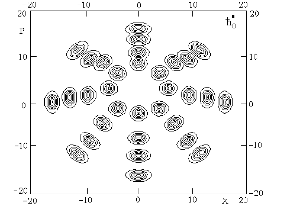
FIG. 2.: Contour plots of the Husimi functions for the exact resonance case, with the resonance number $\mu=4$; $\hbar_{0}=0.12$; $\epsilon=0.002$.

the center of a quantum resonance cell, so that the quantum phase space has the same symmetry as the classical phase space. For $\mu=4$, the symmetry of the Husimi function, shown in Fig. 2, is the same as the symmetry of the classical phase space in Fig. 1. A similar result was demonstrated numerically in Ref. [4] for $\mu=1$. As one can see from Fig. 2, in agreement with Eq. (11), the quantum phase space is symmetric with respect to the substitution: $X\rightarrow-X$. However, there is no exact symmetry with respect to the transformation: $P\rightarrow-P$. The reason is presumably related to our approximation (18) which leads to separation of variables in Eq. (19). This approximation is more valid for the “quasiclassical cells” with $n\gg 1$ than for “quantum cells”, for which the value of $n$ is not large. One can see from Fig. 2, that “quasiclassical cells” are more symmetrical than the “quantum cells”, and the structure of the “quasiclassical cells” is close to the structure of the classical cells shown in Fig. 1. This symmetry of the quantum phase space differs this system from quantum chaotic systems with critical threshold to global chaos.[8]

In summary, the correspondence between the symmetry of the Husimi functions of the QE ground states and the symmetry of the classical phase space has been demonstrated for a degenerate system both analytically and numerically.

I Acknowledgments

We are thankful to D.F.V. James and G.D. Doolen for useful discussions. The work of V.Ya.D. and D.I.K. was partly supported by the Russian Foundation for Basic Research (Grants No. 98-02-16412 and No. 98-02-16237). Work at Los Alamos National Laboratory was partly supported by the National Security Agency, and by the Department of Energy under contract W-7405-ENG-36.

REFERENCES

[1]
G.M. Zaslavsky, R.Z. Sagdeev, D.A. Usikov,
and A.A. Chernikov,
Weak Chaos and Quasi-Regular Patterns, Cambridge Univ. Press,
Cambridge, 1991.