Quantum tomography of the GHZ state

by G. M. D’Ariano^a, M. Rubin^b, M. F. Sacchi^a, and Y. Shih^b,

Abstract. We present a method of generation of the Greenberger–Horne–Zeilinger state involving type II and type I parametric downconversion, and triggering photodetectors. The state generated by the proposed experimental set-up can be reconstructed through multi-mode quantum homodyne tomography. The feasibility of the measurement is studied on the basis of Monte-Carlo simulations.

1 Introduction

A number of proposals for generating the Greenberger–Horne–Zeilinger (GHZ) state [1] has been suggested in the literature [2]. Such kind of state is very interesting as it leads to correlations between three particles in contradiction with the Einstein-Podolsky-Rosen idea of “elements of reality” [3]. In the present contribution we present a scheme for a complete quantum test of a GHZ state of radiation, not just for a simple verification of some GHZ correlations, which do not prove that a true GHZ state has been produced. In fact, the verification of a state-preparation procedure needs a complete state-reconstruction technique, whereas correlation measurements [4] give identical results for very different states of radiation. In this respect, a crucial technique for state-preparation tests is quantum homodyne tomography, in which the detrimental effect of non-unity quantum efficiency of detectors is taken into account ab initio by the reconstruction algorithms.

In the following we propose a method for generating a GHZ state through type II and type I parametric downconversion, and triggering photodetectors. The proposed set-up, although it has low rate of production due to low efficiency for single-photon downconversion, however is the only way to generate a “true” GHZ state, without an additional vacuum component. The scheme allows a tomographic state-reconstruction, whose feasibility here is studied on the basis of Monte–Carlo simulations.

2 Scheme for the GHZ-state generation

The scheme for the generation of the GHZ state is sketched in Fig. 1. A low-gain type-II parametric downconverter is pumped by a strong coherent beam to generate the state

$$|\xi\rangle\simeq(1+2\gamma^{2})^{-1/2}\left[|0\rangle+\gamma\left(|1f_{e},1g_{o}\rangle+e^{i\varphi_{1}}|1f_{o},1g_{e}\rangle\right)\right]\;,$$ (2.1)

in the four radiation modes $f_{e,o}$ and $g_{o,e}$, where $o,e$ represent ordinary and extraordinary polarizations, $\gamma$ denotes the effective coupling depending on the pump strength and the nonlinear susceptibility of the crystal, $|0\rangle$ and $|1a\rangle$ represent the vacuum and the single-photon Fock state for mode $a$, respectively.

Figure 1: Sketch of the experimental set-up for generating the GHZ state. A low-gain type-II parametric downconverter is pumped by a strong coherent beam and generates the state in Eq. (2.1). Two further downconversion processes in type I nonlinear crystals excite modes $a_{o,e},\,b_{o,e},\,c_{o,e}$ and $d_{o,e}$. $\lambda$ and PBS denote a wave plate and a polarizing beam splitter, respectively. The photodetector in the lower part of the scheme collapses the field modes in the state of Eq. (2.9). The photodetector in the upper part checks if the second photon in one of the modes $f_{e,o}$ has been split in the first crystal. The resulting state is a mixture of a Fock state in modes $c_{o,e}$ and of a GHZ state [see Eq. (2.13)], the weights of the two components depending on the effective gain of crystal A and on the quantum efficiency of detector D1.

The state $\xi$ at the output of the first crystal is then impinged on two type-I nonlinear crystal A and B. In this case no classical pump is used and the dynamics must be evaluated without the parametric approximation used to derive Eq. (2.1). For example, the unitary evolution describing crystal A is given by

$$\hat{U}_{A}=\exp{\left[\chi_{A}\left(a_{o}^{{\dagger}}b_{o}^{{\dagger}}f_{e}+e^{i\varphi_{A}}\,a_{e}^{{\dagger}}b_{e}^{{\dagger}}f_{o}-\hbox{h.c.}\right)\right]}\;,$$ (2.2)

$\chi_{A}$ being proportional to the nonlinear susceptibility of the medium. An analogous expression can be written for the crystal B. For simplicity, we assume in the following $\chi_{A}=\chi_{B}\equiv\chi$. The state at the output of the couple of type-I crystals is given by

$$\hat{U}_{A}\hat{U}_{B}|\xi\rangle=(1+2\gamma^{2})^{-1/2}\{|0\rangle+$$

$$\gamma[(\cos\chi|1f_{e}\rangle+\sin\chi|1a_{o},1b_{o}\rangle)(\cos\chi|1g_{o}\rangle+\sin\chi|1c_{e}\,1d_{e}\rangle)+$$

$$e^{i\varphi_{1}}(\cos\chi|1f_{o}\rangle+e^{i\varphi_{A}}\sin\chi|1a_{e},1b_{e}\rangle)(\cos\chi|1g_{e}\rangle+e^{i\varphi_{B}}\sin\chi|1c_{o}\,1d_{o})\rangle]\}\;.$$ (2.3)

As shown in Fig. 1, a wave plate and a polarizing beam splitter act respectively on modes $c_{e,o}$ and $d_{e,o}$ according to the unitary transformations

$$\left\{\begin{array}[]{l}c_{e}\longrightarrow\ c_{o}\\ c_{o}\longrightarrow-c_{e}\end{array}\right.\;,\qquad\quad\left\{\begin{array}[]{l}d_{e}\longrightarrow(d_{e}+d_{o})/\sqrt{2}\\ d_{o}\longrightarrow(d_{o}-d_{e})/\sqrt{2}\end{array}\right.\;.$$ (2.8)

When photodetector D2 reveals one photon after the polarizing beam splitter, one is guaranteed that two photons have been created in the type-II crystal and that the photon impinging on crystal B has been split. This occurs with probability $P_{\Phi}=\eta_{2}(\gamma^{2}\sin^{2}\chi)/(1+2\gamma^{2})$, $\eta_{2}$ being the quantum efficiency of photodetector D2. The corresponding reduced state $|\Phi\rangle$ writes

$$|\Phi\rangle = \frac{1}{\sqrt{2}}[\cos\chi(|1f_{e}\,1c_{o}\rangle-e^{i(\varphi_{1}+\varphi_{B})}|1f_{o}\,1c_{e}\rangle)$$ (2.9)

$$+ \sin\chi(|1a_{o}\,1b_{o}\,1c_{o}\rangle-e^{i(\varphi_{1}+\varphi_{A}+\varphi_{B})}|1a_{e}\,1b_{e}\,1c_{e}\rangle)]\;.$$

Photodetector D1 in the upper part of the scheme monitors the splitting of the photon impinging on crystal A. When such detector, characterized by quantum efficiency $\eta_{1}$, reveals the lack of the “pumping” photon, the resulting output state finally reads as the following mixture

$$\hat{\varrho}=\left\{\begin{array}[]{ll}\;\frac{1}{\sqrt{2}}(|1a_{o}\,1b_{o}\,1c_{o}\rangle-e^{i(\varphi_{1}+\varphi_{A}+\varphi_{B})}|1a_{e}\,1b_{e}\,1c_{e}\rangle)&\ \ p_{1}=\frac{\sin^{2}\chi}{1-\eta_{1}\cos^{2}\chi}\\ |1c_{o}\rangle&\ \ p_{2}=\frac{(1-\eta_{1})\cos^{2}\chi}{2(1-\eta_{1}\cos^{2}\chi)}\\ |1c_{e}\rangle&\ \ p_{3}=p_{2}\end{array}\right.\;$$ (2.13)

The overall probability $P_{\varrho}$ of generating the mixture in Eq. (2.13) is given by $P_{\varrho}=P_{\Phi}(1-\eta_{1}\cos^{2}\chi)$. One easily recognizes in the first component of the mixed state in Eq. (2.13) the GHZ state for a suitable arrangement of the phases, namely for $\varphi_{1}+\varphi_{A}+\varphi_{B}=\pi$.

3 Multi-mode tomographic measurement

Quantum homodyne tomography is the first quantitative technique for measuring the matrix elements of the radiation density operator [5, 6], which is now used in optical labs [7]. Single-mode homodyne tomography can be generalized to any number of modes. However, such a simple generalization needs a separate measurement for each mode, which cannot be achieved when modes are not spatially separated. For this reason, in Ref. [8] it has been proposed a general method for measuring an arbitrary observable of a multi-mode electromagnetic field, using homodyne detection with a single local oscillator. Such method is a natural application of a recent group-theoretical approach to quantum tomography [9]. In the following we recall the main results, providing the rule to evaluate the “unbiased estimator” for a generic (M+1)-mode operator. The quantum expectation value of the operator can be obtained for any unknown state of radiation through an average of such estimator over homodyne outcomes that are collected using a single local oscillator by scanning different linear combinations of modes on it. The quadrature operator to be measured is given by $\hat{X}({\bf\theta},{\bf\psi})=[\hat{A}^{{\dagger}}({\bf\theta},{\bf\psi})+\hat{A}({\bf\theta},{\bf\psi})]/2$ with $\hat{A}({\bf\theta},{\bf\psi})=\sum_{l=0}^{M}e^{-i\psi_{l}}u_{l}({\bf\theta})a_{l}$. The vector $\vec{u}(\theta)$ represents a point on the Poincaré hyper-sphere (for the explicit parametrization see Ref. [8]). By scanning the values of $\psi_{l}\in[0,\pi]$ and $\theta_{l}\in[0,\pi/2]$, all possible linear combinations of modes described by annihilation operators $a_{l}$, with $l=0,\ldots,M$, are obtained. The homodyne outcomes for $\hat{X}({\bf\theta},{\bf\psi})$ can be obtained using a single local oscillator prepared in the multi-mode coherent state $\otimes_{l=0}^{M}|\gamma_{l}\rangle$ with $|\gamma_{l}\rangle=e^{i\psi_{l}}u_{l}(\theta)K/2$, where $K\gg 1$. The expectation value for a given operator $\hat{O}$ is evaluated as follows

$$\langle\hat{O}\rangle=\int\mbox{d}\mu[{\bf\psi}]\int\mbox{d}\mu[{\bf\theta}]\,\int_{-\infty}^{+\infty}\mbox{d}x\,p_{\eta}(x;{\bf\theta},{\bf\psi})\,{\cal E}_{\eta}[\hat{O}](x;{\bf\theta},{\bf\psi})\;,$$ (3.14)

where $p_{\eta}(x;{\bf\theta},{\bf\psi})$ denotes the homodyne probability distribution of the quadrature $\hat{X}({\bf\theta},{\bf\psi})$ for quantum efficiency $\eta$, and the function ${\cal E}_{\eta}[\hat{O}](x;{\bf\theta},{\bf\psi})$ of $x$, $\{\theta_{l}\}$, $\{\psi_{l}\}$ has the following analytic expression

$${\cal E}_{\eta}[\hat{O}](x;{\bf\theta},{\bf\psi})=\frac{\kappa^{M+1}}{M!}\int_{0}^{+\infty}\mbox{d}t\,e^{-t+2i\sqrt{\kappa t}x}\,t^{M}\,\mbox{Tr}\{\hat{O}\hbox{\bf:}\exp[-2i\sqrt{\kappa t}\hat{X}({\bf\theta},{\bf\psi})]\hbox{\bf:}\}\;,$$ (3.15)

with $\kappa=2\eta/(2\eta-1)$. In Eq. (3.15) we used the notation

$$\int\mbox{d}\mu[{\bf\psi}]\doteq\prod_{l=0}^{M}\int_{0}^{2\pi}\frac{\mbox{d}\psi_{l}}{2\pi}\;,\qquad\int\mbox{d}\mu[{\bf\theta}]\doteq 2^{M}\,M!\prod_{l=1}^{M}\int_{0}^{\pi/2}d\theta_{l}\,\sin^{2(M-l)+1}\theta_{l}\cos\theta_{l}\;.$$ (3.16)

For any given operator $\hat{O}$ Eq. (3.15) provides the “unbiased estimator” to be averaged over all homodyne outcomes for the quadrature $\hat{X}({\bf\theta},{\bf\psi})$ of all modes in order to obtain the ensemble average $\langle\hat{O}\rangle$ for any unknown state of radiation. Eq. (3.14) can be specialized to the matrix element $\langle\{n_{l}\}|\hat{R}|\{m_{l}\}\rangle$ of the full joint density matrix. This will be obtained by averaging the following estimator [8]

$${\cal E}_{\eta}[|\{m_{l}\}\rangle\langle\{n_{l}\}|](x;{\bf\theta},{\bf\psi})=e^{-i\sum_{l=0}^{M}(n_{l}-m_{l})\psi_{l}}\,\frac{\kappa^{M+1}}{M!}\prod_{l=0}^{M}\left\{[-i\sqrt{\kappa}u_{l}({\bf\theta})]^{\mu_{l}-\nu_{l}}\sqrt{\frac{\nu_{l}!}{\mu_{l}!}}\right\}$$

$$\times\int_{0}^{+\infty}\mbox{d}t\,e^{-t+2i\sqrt{\kappa t}x}\,t^{M+\sum_{l=0}^{M}(\mu_{l}-\nu_{l})/2}\prod_{l=0}^{M}L_{\nu_{l}}^{\mu_{l}-\nu_{l}}[\kappa u_{l}^{2}({\bf\theta})t]\;,$$ (3.17)

where $\mu_{l}=\mbox{max}(m_{l},n_{l})$, $\nu_{l}=\mbox{min}(m_{l},n_{l})$, and $L_{n}^{\alpha}(z)$ denotes the customary generalized Laguerre polynomial of variable $z$.

4 Numerical results

The tomographic measurement on the state in Eq. (2.13) can be suitably performed by varying randomly the phases and the polarizations for the couples of modes $a_{o,e}$, $b_{o,e}$ and $c_{o,e}$ and then collecting homodyne outcomes by using three local oscillators. Such an experimental arrangement represents an intermediate way of using the multi-mode tomographic method of Sect. 3, and the usual method based on the product of single-mode estimators. By using the estimator in Eq. (3.17) one can measure tomographically the expectation value of the projector $|\phi\rangle\langle\phi|$ with

$$|\phi\rangle\equiv\frac{1}{\sqrt{2}}\left(|1a_{o}\,1b_{o}\,1c_{o}\rangle+e^{i\phi}|1a_{e}\,1b_{e}\,1c_{e}\rangle\right)\;$$

on the state $\hat{\varrho}$ in Eq. (2.13) and compare the result with the theoretical value, namely

$$C(\phi)\equiv\langle\phi|\hat{\varrho}|\phi\rangle=\frac{1}{2}\,p_{1}\,\left[1-\cos(\phi-\varphi)\right]\;$$ (4.18)

We report in Fig. 2 the results of some Monte-Carlo simulations of the tomographic measurement of $C(\phi)$ in Eq. (4.18).

                  

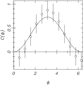
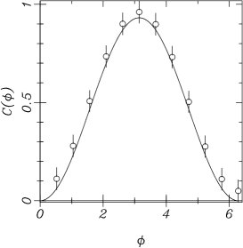
Figure 2: Tomographic measurement of $C(\phi)$ in Eq. (4.18) for $\varphi=0$. On the left: $\eta=0.85$, $\chi=0.3\,\pi$, $N=6\times 10^{6}$. On the right: $\eta=0.9$, $\chi=0.4\,\pi$, $N=1.7\times 10^{7}$.

In the simulations the quantum efficiency of detectors D1 and D2 is $\eta_{1}=\eta_{2}=30\%$ and the phase $\varphi$ in the state (2.13) is $\varphi=0$. The values of the quantum efficiency $\eta$ of homodyne detectors, the coupling $\chi$ of type-I downconvertors, and the number $N$ of simulated homodyne data are reported in the caption of the figures. The results of the simulations show that for homodyne detectors with quantum efficiency $\eta=85\%$ one needs about $10^{7}$ data to reconstruct the state with relatively small statistical error. The experimental values compare very well with the theoretical ones. The bars represent the statistical error, whereas the solid line is the theoretical value of $C(\phi)$. In each plot, all points are obtained by the same sample of data which causes the evident correlation between the statistical deviations.

References

References

• [1] D. M. Greenberger, M. Horne, and A. Zeilinger, in Bell’s Theorem, Quaantum Thoery, and Conceptions of the Universe, M. Kafatos, Ed. (Kluwer, Dordrecht 1989) pp. 69-72.
• [2] See T. E. Keller, M. H. Rubin, Y. H. Shih, and L. Wu, Phys. Rev. A 57, 2076 (1998), and references therein.
• [3] A. Einstein, B. Podolsky, and N. Rosen, Phys. Rev. 47, 777 (1935).
• [4] D. Bouwmeester, J. Pan, M. Daniell, H. Weinfurter, and A. Zeilinger, Phys. Rev. Lett. 82, 1345 (1999).
• [5] G. M. D’Ariano, C. Macchiavello, and M. G. A. Paris, Phys. Rev. A 50, 4298 (1994).
• [6] G. M. D’Ariano, in Quantum Optics and the Spectroscopy of Solids, T. Hakioǧlu and A. S. Shumovsky, Eds. (Kluwer, Dordrecht 1997) pp. 139-174.
• [7] G. Breitenbach, S. Schiller and J. Mlynek, Nature 387, 471 (1997).
• [8] G. M. D’Ariano, P. Kumar, and M. F. Sacchi, unpublished.
• [9] G. M. D’Ariano, Acta Physica Slovaca 49, 513 (1999).