On the observation of decoherence with a movable mirror

Abstract

Following almost a century of debate on possible ‘independent of measurement’ elements of reality, or ‘induced’ elements of reality - originally invoked as an ad-hoc collapse postulate, we propose a novel line of interference experiments which may be able to examine the regime of induced elements of reality. At the basis of the proposed experiment, lies the hypothesis that all models of ’induced’ elements of reality should exhibit symmetry breaking within quantum evolution. The described symmetry experiment is thus aimed at being able to detect and resolve symmetry breaking signatures.
Pacs numbers: 03.65.Bz, 42.50.Vk, 42.50.Dv.

I Introduction

The loss of the ability to consistently use the word particle (referring to a classical point of mass), is of course one of the well known implications of quantum mechanics, and stands at the base of what has been named the ‘measurement problem’. Instead, we make use of a mathematical entity called the wave function, which is allowed superpositions which cannot describe our classical notion of reality. This is perhaps most readily exhibited in the double slit experiment. Indeed it was Feynman who described the double slit experiment as ”…it contains the only mystery”[1]. It is also a matter of general knowledge that many of the important contributors to the theory were not satisfied with this state of affairs. They felt that some level of independent reality does in fact exist, and connects to quantum expectations through some set of local or non-local hidden variables. Just to mention a few, de-Broglie for example, tried to formulate alternatives such as the ‘guiding wave’ or the ‘double solution’ models, which were, by his own admittance, unsuccessful. Nevertheless, until his last days, he continued to believe that a theory maintaining some sort of particle independent reality should be found [2]. Bohm, went a step further by publishing a consistent formalism which enables the existence of a particle, while reproducing standard quantum expectations [3]. Indeed some, such as Bell, have taken the view that Bohm’s success presents a superior interpretation, while others thought differently [4]. Einstein with the EPR paradox, Schrödinger with the cat enigma, and other important contributors, were also uncomfortable. We refer the interested reader to some of the many available textbooks on the interpretation of the past and possibilities of the future regarding quantum theory [5].

Simply stated, the measurement problem may be described as follows: If there are two possible pointer positions (in the measuring apparatus), the superposition principle maintains that any superposition of those two pointer positions must also be a possible state. However, such superposition states of macroscopic pointers have never been observed [6]. In the language of the above single particle double slit experiment: The superposition principle does not allow us to use the word particle if we are to describe the evolution of the quantum system. However, the outcome of the experiment necessitates the use of the word particle in contradiction to the superposition principle. Even if one accepts Bohr’s escape route, which divided the world into quantum and classical, one is left with a fuzzy, impossible to define, border between the two.

A second class of models attempting to resolve the measurement problem invokes ‘induced reality’ rather than ‘independent reality’. Namely, classical reality as an outcome of processes, which depend on parameters such as time and mass (or number of particles). One example of such a model would be the spontaneous localization through the GRW (Ghirardi, Rimini and Weber) mechanism and its successors [7]. Another example is what Folman and Vager described as the ‘non-passive Bohmian particle’ [8], which Bohm described as a particle having influence on the wave function ”…so that there will be a two way relationship between wave and particle” [9]. In this scenario, the wave function, which determines the evolution of the system, is gradually distorted by the particle and its location – away from the form of superposition. There are numerous other hypothesized models such as Gravity based induced decoherence (see Penrose [10]), but perhaps the most well known model of this class of ‘induced reality’ models, is that of a ”collapse” due to the coupling to the environment. This is usually referred to as Decoherence, which states in essence that the reduced density matrix Von Neumann called for (having no off diagonal elements) may be arrived at naturally through the entanglement of the system and the detector to the environment (see Zurek [11]). In addition to the usual parameters of time, mass and spatial separation (which are needed if we are to explain our observations), Decoherence correlates the loss of coherence to the coupling onto the environment.

The question we would like to address in this note, is how may we try and experimentally investigate the second class of models (where by decoherence, we will be referring to the important x space), so that their general validity would be asserted, and furthermore, how may we possibly differentiate between them.

II The experimental problem

There are two major experimental problems concerning the observation of localization as a function of time, mass and the variation of the coupling to the environment.

Problem I:It is hard to observe a quantum system without coupling to it and initiating unwanted decoherence as part of the measuring process. In such a measurement, decoherence and the collapse postulate cannot be differentiated, since the more we couple the environment (e.g. through our pointer) to the observed system, the more we know about that system, and the more dephasing we expect from the collapse postulate [12]. Here, we mention the collapse postulate in the sense of our consciousness gaining knowledge about the system.
Resolution I:Use non-demolishing measurements in which the system’s unitary evolution in the base of your choice (in our case it will always be x), is not affected by the measurement.

Here, it is interesting to note, that following a suggestion for a gravitationally induced collapse model [10], Schmiedmayer, Zeilinger and colleagues have also investigated the idea of monitoring the behavior of a coherent system in order to observe decoherence [13]. They made the point that any ‘welcher weg’ information would have to be erased or not invoked in the first place, for such an experiment to be performed. As will be shown in the following, this is exactly the idea behind our proposed experiment and why we consider it to be non-demolishing.

Problem II:Traditionally, observed coherent systems in a state of superposition are particles, atoms or molecules. These are either too light to observe localization in the time frame of the experiment, or, their mass is fixed, making it hard to determine the proportionality of localization to mass. Furthermore, particles in well defined states of spatial superposition, are usually in motion, which makes the control of their environment a hard task.
Resolution II:Keep particles only as probe while turning the set-up into the observed system, which is in a well defined spatial superposition, with a variable mass and environment.

Finally we note that the affect of the environment, as well as other parameters, on localization has long been the subject of experimental interest, but as far as we know, with no conclusive results. For example, one such on going experimental effort concerns the handedness of chiral molecules [14]. Another experiment investigated decoherence of an ‘atom-cavity field’ entangled state, where the macroscopic element was that of the phase difference between the cavity fields [15]. Recently, several schemes have suggested ways to directly investigate macroscopic objects [16]. In this context, micro movable mirrors (which are also discussed in this paper) have also been discussed extensively [17]. This, however, as far as we know, only in the context of cavities. In the following we present what is to the best of our knowledge a novel type of experimental procedure in the context of localization, which may shed new light on the processes initiating it. It relates to the issue of symmetry in quantum phenomena, which is an underlying feature of the theory. Namely that the difference between classical and quantum states is that the phase between possible positions is lost, and hence symmetry in space may exist between probabilities but not amplitudes.

III The experimental assumptions

In ref. [8], Folman and Vager proposed to incorporate the two experimental resolutions described above by utilizing a symmetry experiment with a movable mirror, to observe localization and decoherence. Their point was that localization could be observed, not only by the breaking of energy conservation (producing photon emission) – as suggested by Pearle and Squires [7], but also by the breaking of symmetry. However, they mainly dealt with issues pertaining to unfavorable empty wave models and gave little consideration to the experimental feasibility. In this note, we expand the idea of the symmetry experiment to include all models of the second type. We also include different versions of the experiment, which may be more realizable and conclusive. Finally, we also present initial calculations to examine the experimental feasibility.

Before describing the experiment, we lay down the foundation by emphasizing several assumptions that cannot, to the best of our understanding, be avoided. For convenience, we first deal with independent collapse mechanisms such as the GRW mechanism, and then move on to the more subtle question of non-independent collapse mechanisms.

Working assumption I: The invoking of localization, via models of the second type, destroys amplitude (wave function) symmetry, even when we have not gained any knowledge of which of the possible x states has been occupied. Namely, symmetric or anti-symmetric states become asymmetric. Consequently, eigen-states of Parity are lost. For example, it is well known that for localized chiral molecules having well defined handedness, Parity is not a good quantum number. In general, if this working assumption were not valid, then it would follow that a classical reality or at the very least the change of the wave function, independent of our consciousness, has not been invoked by this second class of models, although this was their main goal. Indeed, symmetry of the wave function must be lost as the loss of the relative phase is an essential part of all localization schemes.

Working assumption II: Measuring whether Parity is a good quantum number of the system (or even collapsing the system into an eigen-state of Parity) does not localize the system (in the sense of the collapse postulate), as it gives us no knowledge what so ever concerning its location. More so, even in the context of models where localization is independent of our knowledge, a measurement of Parity does not decohere the system (in x space). This working assumption is self evident as the spatial spread of the wave function remains unchanged by the Parity operator. Using once again the example of chiral molecules, measuring Parity does not induce handedness. In another example, as shown by Scully et al. [18], sending excited atoms through optical cavities which serve as ’welcher weg’ detectors, does not destroy the interference pattern if the only knowledge gained is that a photon has been released (i.e. both cavities were exposed to the same photon detector), and no knowledge is available regarding at which cavity the photon has been released. As photon emission can only be done in conjunction with a symmetric atom wave function, the ‘quantum eraser’ experiment shows us that measuring the Parity of the atomic wave function, does not destroy its coherency.

Working assumption III: There are no other possible causes for symmetry breaking aside from the hypothesized localization. Namely, if the set-up is symmetric and the Hamiltonian conserves Parity (we neglect the weak force), any sign of symmetry breaking must be due to localization. Again, if this was not so, we would have observed symmetry breaking long ago, due to a breaking term in the interaction.

Following working assumptions I, II & III, we set out to search for symmetry breaking effects.

IV The experiment

The first stage of the experiment includes the preparation of a symmetric initial particle wave function $\Phi_{i}$. This may be done by the apparatus presented in figure  1. D1 and D2 are two particle detectors (if needed, with the ability to measure the particle’s energy). $S$ is the particle source. The phase shifter ($PS$) cancels the phase difference introduced by the beam splitter ($BS$), between the phase of the transmitted wave and that of the reflected. We of course assume a perfect $50\%/50\%$ $BS$ and a $PS$ which is invariant to changes (as is the $BS$) in the wave number. The same apparatus also serves as the measurement apparatus with Parity eigen-states.

The interaction region may hold several types of experiments.

a. The closed loop interferometer:

This interferometer has the distinct advantage of ensuring symmetry, as its two optical paths are one and hence identical.

In the simplest case, where we set out to examine induced collapse independent of the environment, the interaction region may stay empty.

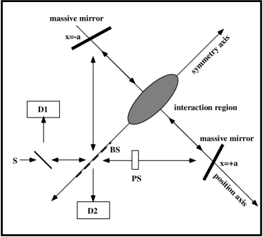
FIG. 1.: The closed loop interferometer. As the interaction region C is transparent, both paths are identical as they are one of the same. S, D1, D2, BS, PS are the particle source, the two detectors, the beam splitter and the phase shifter, respectively. The eigen-states of the measuring system are Parity eigen-states. While transversing the apparatus, the initial symmetric wave function is exposed to the influence of the relevant parameters such as time, spatial separation, and environment, or any other symmetric interaction which we place at the interaction region C. There is no reason for the outgoing wave function to loose its initial symmetry and hence we expect no ’click’ in detector D2, unless loss of coherence due to localization has occured.

The two important parameters are time and mass (or number of elementary particles). Mass could be controlled by the size of the particles we send into the interferometer, and time by their velocity and the size of the interferometer.

Dependence of localization on the environment, may be examined by introducing a symmetric interaction which would keep the Hamiltonian invariant to space inversion along the position axis (e.g. magnetic or electric field or modulating crystal).

In all these cases, a ’click’ in D2 would mean that the single particle initially arriving from $S$ with a symmetric $\Phi_{i}$ has now transformed to a final $\Phi_{f}$ which is anti-symmetric or asymmetric. As there are no reasons for $\Phi_{f}$ to be anti-symmetric (see assumption III) we conclude that $\Phi_{f}$ is asymmetric. In the single particle case some of the asymmetric photons would end up in detector D2, telling us that the particle was localized. This could be verified by repeating the experiment with a multi-photon pulse and observing hits on both detectors. As the collapse postulate cannot be responsible for the observed symmetry breaking (see assumption II), we conclude that we have observed induced localization (see assumption I).

b. The open loop interferometer:

If we are not able to achieve coherent symmetric states with very massive particles (needed if we are to observe induced localization on the time scale in which the particles transverse the apparatus), or if we are unable to satisfactorily control the particles’ environment while they are in motion, we would have to resort to a more complex experimental scheme which we describe here as the open loop interferometer. Different from the previous interferometer, here, the interaction region is blocked by a second symmetric quantum system. In this scheme, we loose the simplicity of having only massive reflections but we gain the possibility of observing a quantum object in a localized potential, for long periods of time and with the ability to control its mass and environment. Consider, for example, the set-up of figure 2.

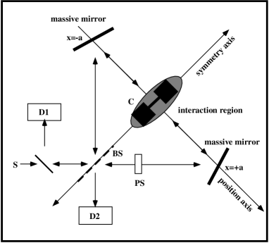
FIG. 2.: The open loop interferometer. Here, in addition to what has been described in figure 1, we position a two sided foil mirror, held in an harmonic potential, into the interaction region C. Hence, we entangle the transversing particle to the state of the set-up, which is also in a well defined quantum state with a well defined spatial uncertainty. Thus, we are able to examine the quantum evolution of a macroscopic system. Using Parity eigen-states to measure the state of the outgoing particle, we learn about the decoherence of the set-up, without affecting it.

Here, a mirror has been placed in the interaction region. In this example, the mirror in the interaction region ($C$) is actually a two sided reflecting foil which is in an harmonic oscillator potential. Neglecting inner degrees of freedom, such as those corresponding to the Debye-Waller factors (since it is known that these factors also exist in massive mirrors but still they reflect coherently), we take account only of the center-of-mass of the foil, and note that it is in a Parity eigen-state (say, the even ground state $\Psi_{i}$). We further note that $\Psi_{i}$ is symmetric with respect to the same symmetry axis as $\Phi_{i}$. Namely, they are both symmetric with respect to the axis that lies in the plane of the beam splitter, which is also the plane of the average position of the foil.

As the total initial wave function $\Omega_{i}~{}=~{}\Phi_{i}~{}\otimes~{}\Psi_{i}$ is symmetric and as the Hamiltonian is Parity conserving and invariant under the combined two reflections of the x’,x” coordinates of the two wave functions, the final total wave function $\Omega_{f}$ must also be symmetric and hence it may be defined as

$$\Omega_{f}~{}=~{}\sum{\Phi_{s}~{}\otimes~{}\Psi_{s}~{}+~{}\Phi_{as}~{}\otimes~{}\Psi_{as}}$$ (1)

where ‘s’ and ‘as’ stand for symmetric and anti-symmetric, and the summation is over all possible foil states (The latter is a general consequence of Parity conservation. For a formal derivation with the specific coherent reflection Hamiltonian, see appendices). We note that these arguments are independent of the mass of the foil $C$.

Changing the observation time, or the environment or the mass of the foil, would allow us to investigate the process of induced localization. Registering a ’click’ in detector D2 with an energy that is not in accordance with the energy gap between the foil’s initial symmetric state and one of the odd states, will indicate the occurrence of symmetry breaking and of induced localization. Again, using a multi-photon pulse may enable a complementary check to the single photon probe.

Let us add here that although we leave the important question of preparation for future publications, we would like to note that preparing the foil in a pure quantum state, is for some cases not a necessary pre-condition. Any well defined probability distribution of state occupation, will sufice. For example, reference [16] advocates the appropriateness of the thermal state of a moving mirror, as a well defined initial quantum state.

Finally we note, that changing the set-up slightly, one may prohibit localization signals from detector D2 (i.e. only anti-symmetric excitation events would ‘click’ at D2), and hence establish yet another complementary check on the source of the deviations. As an example of such an apparatus, we present the set-up of figure 3. Here, massive mirrors $A$ and $B$ maintain the loop actually closed.

We end this section by noting that the above presented experimental procedure should be able to investigate any model in which decoherence is also a function of mass and time. As these parameters are essential in all models of the second type, we conclude that the symmetry experiment may be utilized to investigate the full range of models of this class.

FIG. 3.: The semi-closed loop interferometer. Here, we add two massive mirrors to the set-up of figure 2, so as to close the interferometer loop. This, makes the set-up insensitive to localization signals while still sensitive to quantum excitations of the mirror foil, hence enabling a further verification of our understanding of the results.

V Some numbers

Let us make some initial calculations for the open loop interferometer, to show what kind of experimental procedure would be needed to realize this experiment.

We start by the demand that the wavelength $\lambda$ of the probing particle would be much smaller than the localization position $X_{loc}$ which is of the order of the width $W$ of the ground state at interaction region $C$ (If this were not so, the localization signal would be suppressed as $\frac{I_{2}}{I_{1}}=\tan^{2}(4\pi\frac{W}{\lambda})$ where $I_{1}$ and $I_{2}$ are the photon intensities at detectors D1 and D2. A derivation is given in appendix A). For now, let us then assume an harmonic potential so that $W=\sqrt{\hbar(n+\frac{1}{2})/(\frac{1}{2}m\omega)}>>\lambda$ (which only differs by a factor $\sqrt{2}$ from the frequently used $W=\sqrt{<x^{2}>}$).

We would first like to see if we are able to isolate through energy measurements of the outgoing particles, those ‘clicks’ at D2 which do not originate from the standard odd excitations of the foil mirror. If we take for example the photon as a probing particle, and assume that we are able to use light from x-ray to red at a wavelength of $0.1-1000nm$, and system $C$ is say in the ground $n=0$ state, we find that for x-ray (red):

$$\sqrt{\frac{\hbar}{m\omega}}>>0.1nm(1000nm)~{}or~{}m\omega<<10^{-14}(10^{-22})$$ (2)

The needed energy resolution $\frac{\hbar\omega}{E_{\gamma}}$ in order to be able to take account only of non excitation events, as a function of the number of particles in the foil, is presented in figure  4.

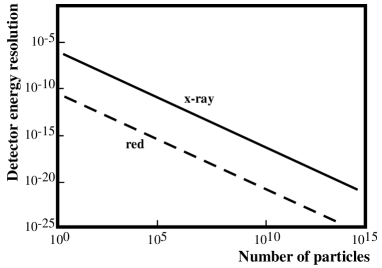
FIG. 4.: Needed energy resolution $\frac{\hbar\omega}{E_{\gamma}}$ as a function of the number of foil nucleons, for the two examined extremes of the feasibly used light spectrum.

Demanding a detector energy resolution of say $10^{-13}$, the harmonic frequency $\omega$ should be less than $10^{5}$, which would mean for the preferred x-ray, an oscillating mass of $10^{-19}kg$ or $10^{8}$ particles. This would mean a $10^{-7}$ collapse probability per second (If one is to take for example a GRW factor of $10^{-15}$ collapse probability per particle per second [19]). To observe ten events one would need three parallel set-ups continuously performing a one second experiment for the length of a year. Indeed, it seems that with present available energy detection resolution, it would be very hard to perform this experiment, while maintaining sensitivity to the full range of possible second class models and parameter values [20].

Following the above conclusion, let us now examine whether perhaps energy measurements would not be needed since excitations will be suppressed by the maximally allowed energy transfer. We note that the maximum energy transfer by the photon cannot exceed that allowed by momentum conservation, namely: $\frac{2(\hbar k)^{2}}{m}\approx\frac{8\times 10^{-47}}{m}$ which would mean in the case of a $10^{8}$ nucleon oscillator, an approximate transfer of $8\times 10^{5}Hz$. This should be compared with the $10^{4}Hz$ maximally allowed energy spacing, under condition (2). This ratio between the maximum transferred energy by momentum conservation and the maximally allowed harmonic energy spacing is constant for all masses and wavelengths, and has the value of $\frac{2(\hbar k)^{2}}{m}/\frac{\hbar^{2}}{m\lambda^{2}}=8\pi^{2}$. Namely, momentum conservation does not prohibit the harmonic oscillator system from being excited to at least the first odd level.

As we have taken $|k_{i}|$ and $|k_{f}|$ to be identical, the latter calculation is of course only valid in the limit of massive objects which due to their mass do not receive significant recoil energy. For exact numbers, we would need to make the quantum calculation which is simple enough. The probability for the foil not to be excited is simply the well known Debye-Waller factor $P_{0\rightarrow 0}$ which is for the case of the x-ray, and again under condition (2), smaller than

$$\exp(-\hbar^{2}(2k)^{2}/2m\hbar\omega)=\exp(-8\hbar\pi^{2}/\lambda^{2}~{}10^{-14})\approx 10^{-35}$$ (3)

(The full calculation may be found in appendix B). We see that the energy transfer can actually be equal to many times the harmonic energy spacing. Hence, we come to the conclusion that working within the ‘high resolution’ $W>>\lambda$ regime and with non-excitation events, is not feasible (this is true for both x-ray and red light).

Finally, one may then ask: Can we avoid the need for energy measurement altogether by simply preparing an experimental procedure in which $P_{0\rightarrow n(odd)}$ (i.e. the expected excitation signal at D2) is well known? Namely, by knowing what the expected ‘noise’ in D2 is (i.e. the anti-symmetric photons coming from excitation events), one can differentiate between the signal at D2 and the ‘noise’. However, for the experiment to be feasible, one must make sure that the noise does not overwhelm the signal. Hence, we need to calculate the values of the ratio

$$R=\frac{1-P_{0\rightarrow n=0,2,4,..}}{I_{2}/(I_{2}+I_{1})}$$ (4)

where,

$$\frac{I_{2}}{I_{2}+I_{1}}=\int_{-\infty}^{+\infty}f(X_{loc})\sin^{2}(4\pi\frac{X_{loc}}{\lambda})dX_{loc}$$ (5)

and where,

$$f(X_{loc})=\Psi_{0}^{\dagger}(X_{loc})\Psi_{0}(X_{loc})$$ (6)

One more possibility to bypass the need for identifying the photons via an energy measurement, is to use multi-photon pulses, as described before.

In the following section we investigate these two propositions.

VI The proposed experimental procedure

From the previous section it is understood that for lack of very small line width sources and very high resolution energy detectors, it seems we are left with two viable experimental procedures, which do not make use of energy measurements:

a. Single photon experiment, where the search will be for deviations from the calculated ratio $I_{1}/I_{2}$ between symmetric and anti-symmetric photon final states. Here, many repetitions of the same single photon experiment will enable us to directly measure the ratio between symmetric and anti-symmetric final states, which in turn is a consequence of the excitation probabilities. This experiment will enable us to measure the excitation probabilities in a quantum macroscopic system and to be sensitive to deviations which are due to localization.

b. Multi-photon (pulse) experiment, where $I_{1}/I_{2}$ are different for a symmetric outgoing pulse, an anti-symmetric outgoing pulse and an a-symmetric outgoing pulse. Here, a localization event may be detected by the abnormal intensity of a single pulse split at the beam splitter.

Experiment a: To see if this experimental procedure allows for a reasonable signal over noise ratio, and for what values of the parameters it does so, we calculate $R$ as a function of $m,~{}\lambda$ and $\omega$. As mentioned before, we ignore the internal degrees of freedom (based on the coherent reflection of visible light mirrors and x-ray gratings) and treat the center-of-mass motion of the mirror. Namely, as in the Mössbauer effect, there are no excitations of internal degrees of freedom. Whether or not this is a good approximation, depends on the specifics of the incoming wave and the mirror, including its thickness and material (see in the following, discussion regarding the extinction coefficient in section ‘The mirror’). With the above assumption, and in the Lamb-Dicke limit (see full calculation in appendix C), we find $R$ to be

$$\frac{\eta^{2}+(higher~{}orders)}{I_{2}/(I_{2}+I_{1})}$$ (7)

where $\eta$ is the Lamb-Dicke parameter $\sqrt{\frac{E_{r}}{\hbar\omega}}=\frac{4\pi}{\sqrt{2}}W/\lambda$ ($E_{r}$ is the recoil energy), and where we have neglected factors which appear in appendix C.

Of course, whether or not a system is in the Lamb-Dicke limit depends on the chosen experimental parameters. Indeed, the accurate calculation of $R$, which is essential for any experimental realization, will depend heavily on the set-up. Hence, keeping to a general frame, we plot in figure 5 a simple example of the behavior of $R$: the upper bound of $R$, namely,

$$R_{bound}=\frac{1-P_{0\rightarrow 0}}{I_{2}/(I_{2}+I_{1})}$$ (8)

(this simple enough calculation is also presented in appendix C). The rather striking ‘inversion’ in $R_{bound}$ seen in the figure, is dependent on the mass of the foil, its frequency and the frequency of the impinging light, only via the parameter $\eta$! For x-ray and $10^{15}$ particles, the frequency of the foil is $f=\frac{10^{-1}}{\eta^{2}}Hz$. This means that in order to observe the inversion in $R$, one would have to work in the regime of very low frequencies. However, it is expected that the full ’inversion’ presented in figure 5, would not be experimentally observable in any case; as can be readily seen from the Debye-Waller expression in eq. (3), which simply equals $\exp(-\eta^{2})$: $P_{0\rightarrow 0}<10\%(>90\%)$ for $\eta>1.5(<0.3)$. One may then roughly assume that for the first case $1-P_{0\rightarrow 0}\rightarrow 2(1-P_{0\rightarrow n=0,2,4,..})$ since $P_{0\rightarrow 0}\rightarrow 0$ and $P_{0\rightarrow 0,2,4,..}\rightarrow\frac{1}{2}$. Similarly for the second case, $1-P_{0\rightarrow 0}\rightarrow 1-P_{0\rightarrow n=0,2,4,..}$ since $P_{0\rightarrow 0}\rightarrow 1$ and $P_{0\rightarrow 0,2,4,..}\rightarrow 1$. Hence, we find respectively that for $\eta>1.5$: $R\rightarrow\frac{1}{2}R_{bound}$, and for $\eta<0.3$: $R\rightarrow R_{bound}$. Consequently, this means that instead of observing the full ’inversion’ one should be able to observe a peak in the value of $R$ for $\eta$ in the region of $0.9$. This is qualitatively described in figure 5.

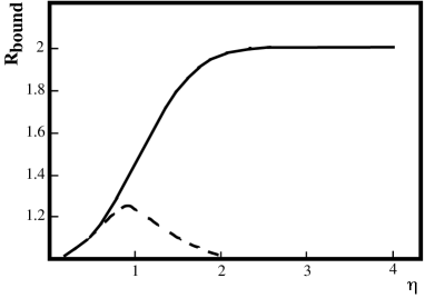
FIG. 5.: $R_{bound}$ as a function of $\eta$, which in turn is a function of the foil mass and frequency, and the wavelength of the light, with the relation $\eta=\frac{4\pi}{\sqrt{2}}W/\lambda=\frac{4\pi}{\lambda}\sqrt{\hbar/2m\omega}$. The dashed line qualitatively presents the general expected form of $R$ (see text). Note that the Lamb-Dicke limit is only valid for $\eta<<1$.

As $R\leq~{}R_{bound}$, the experimental sensitivity for the various values of the experimental parameters, will be better than that indicated by the bound. Observing the above form of the dependence of $R$ as a function of $m$, may serve as yet another verification that the deviations that are observed at detector D2, indeed originate from localizations. For example, for a constant $10Hz$ foil frequency, the range of $0.1<\eta<2$ could be scanned by simply changing the mass of the foil in the range $10^{12}<no.~{}of~{}particles<10^{15}$.

As for red light, one can easily see that for $10^{15}$ particles $f=\frac{10^{-9}}{\eta^{2}}Hz$, which means that although one may perform the experiment with red light (reasonable anti-symmetric ‘noise’ to signal ratio), one is not able to explore the ‘inversion’ regime, as the needed foil frequency would be far below $1Hz$ (which would probably be mechanically hard to achieve. See following section: ”The mirror”), or alternatively, the needed foil mass would be extremely small, and in order to observe decoherence, one would have to maintain a stable and isolated experiment, for long periods of time. Nevertheless, if one has enough statistics, one may try and observe the logarithmic behavior of $R$ for smaller values of the $\eta$ parameter. In any case, it should be once again noted, that as the observation of the ‘inversion’ or logarithmic behavior are mere verifications, the experiment itself could be performed with a large range of light and mirror frequencies.

Finally, we add that although in general, localization times in the different models depend on the number of particles or the mass, some models also take into account the spatial seperation. For our bound mirror foil, the larger the mass, the smaller the ground state size and hence the position uncertainty, which constitutes the seperation between the different possible positions. Thus increasing the mass will on the one hand shorten the decoherence time but on the other hand prolong it. It is therefore clear that the exact parameters needed in order to achieve decoherence on the experimental time scale, are model dependent. However, it is also clear that any model attempting to explain the ’localization of the pointer’ must also predict the localization of our mirror. It remains to adjust the experimental parameters so that the predicted decoherence times are within the experimental time scales.

We now turn to the second possible experiment.

Experiment b: The immediate and clear advantage of a multi-photon pulse experiment, is of course the fact that a single experiment (i.e. one pulse) can detect a localization. The clear signal would be an $I_{2}/I_{1}$ ratio which is classically related to the $X_{loc}$ of the localization. Integrating over all observed localization signals, should of course be in agreement with the density function of the ground state. The important issue at hand is: what would be the signal coming from non-localization events (coherent excitation and non-excitation events).

Let us assume the pulse as being a simple sum of $N$ independent photons. Let us also assume that we are working in the limit where $N\times P_{int}<<1$, where $P_{int}$ is the probability of an inelastic (i.e. excitation) photon-foil interaction. Namely, if a photon inelastically interacts with the foil, the chance of another such interaction in that pulse, is negligible. As we have seen for the Lamb-Dicke limit, this is indeed the case. In this limit we can expect that a maximum of one photon would ’click’ at D2 for every pulse, while for a localization event, we would expect on average many more. We will leave further elaboration regarding this option for a specific note, and simply state that as long as the above assumptions are correct, and as long as the pulse time imitates the single photon experiment in that it is short relative to the period of the oscillator, we expect the multi-photon experiment to have interesting features worth examining.

We now turn to discuss some aspects of the mirror design.

VII The mirror

In the previous paragraphs, we calculated the excitation probability without taking into account the specific features of the mirror. Obviously, a full account of the mirror features has to be made. This is not just a matter of the mirror’s material. The mirror’s thickness may also dominate the ability of the mirror to reflect or to have a wanted ground frequency (e.g. of the order of the example $10Hz$). In the following we present some preliminary classical considerations which will have to be followed when constructing the mirror.

For example, if one takes an atom to have a volume of $10$ cubic Angstrom, then a $1mm^{2}$ mirror, would have a thickness of only $10-1000$ atom layers for $10^{13}$ to $10^{15}$ atoms. The question then arises if such a small thickness can have non-negligible reflectance. Taking perpendicular impinging beams (i.e. parallel and perpendicular polarisations give rise to the same border reflection), and for simplicity ignoring interference between reflections coming from the two mirror bounderies, one should expect reflection from each of them, with a strength of $|(N_{1}-N_{2})/(N_{1}+N_{2})|^{2}$ where $N_{1}$ and $N_{2}$ are the complex indices of refraction of the mirror and its surroundings ($N=n+i\kappa$, where $n$ is the index of refraction and $\kappa$ is usually referred to as the extinction coefficient. If $n/\kappa>>1$, then $\kappa$ may be neglected in the above calculation). From the latter it is clear that in order to reflect, the mirror material must be immersed in an environment with an index of refraction different than its own, or alternatively, when this is hard to achieve such as for x-ray, the mirror should be constructed to Bragg reflect the light. $\kappa$ also affects the internal scattering and heating of the mirror. A small $\kappa$ ensures that the internal absorption $1-\exp(-2k\kappa x)$ will remain small (where $k$ is the wave vector of the incoming wave and $x$ is simply the propagation distance of the wave within the material). Experimental values for the extinction coefficient in the x-ray region are usually of the order of $10^{-6}$ to $10^{-7}$  [21]. Making use of these numbers and a mirror thickness of $100A$, one finds an absorption of less than $1\%$. Of course, a more accurate account should also take into consideration factors like the dependence of the extinction coefficient on temperature, errors rising from roughness and contamination of the mirror surface, etc. [21]. For red light, having an extinction coefficient of about $10$ (for example, metals in the red region), one finds that the absorption for a $100A$ mirror would be above $50\%$ and must therefore be seriously considered.

One should also consider the mechanical properties of such a mirror. Namely, can the mirror be fabricated to have the example frequency of $10Hz$. It is well known that rectangular or circular plates with clamped edges have a fundamental $(0,0)$ mode frequency of order $C_{L}h/L^{2}$ (times $1.654$ or $0.4694$ for rectangular and circular, respectively), where $L$ is the dimension of an oscillating plate of thickness $h$ and $C_{L}=\sqrt{E/\rho(1-\nu^{2})}$ is the velocity of sound in the plate [22]. $E$ is Young‘s Modulus. Taking for example metals, $E$ is in the order of $10-20\times 10^{3}N/m^{2}$, $\rho$ is the density, which for metals is in the order of $10-20\times 10^{3}kg/m^{3}$, and $\nu$ is Poisson‘s ratio, which is $0.3$ for most materials. Taking the thickness to be $100A$ and the mirror to be of dimension $1mm$, one finds that the frequency will be of the order of $10Hz$ as required.

Finally , we discuss environmentally induced decoherence.

VIII Observing environmental Decoherence

Before the end of this paper, we would like to revisit the issue of the work assumptions. The working assumptions, which have been presented in the beginning of the paper, form the underlying logic behind the hypothesis that the symmetry experiment should exhibit sensitivity to all models of the second class. However, the different models of this class have slightly different features and hence require slightly different working assumptions to ensure the sensitivity of the experiment to them. In the beginning of the paper, we started for simplicity with the GRW model. As an example of a different model, of a non-independent collapse nature, we now briefly discuss the environmentally induced collapse model. Here we will simply repeat the three working assumptions for the case of environment related collapses, and note that a fourth assumption should be added:

Working assumption I: The invoking of coherence-loss, via models of the second type, destroys amplitude (wave function) symmetry, even when we have not gained any knowledge of which of the possible x states has been occupied. Namely, symmetric or anti-symmetric states become asymmetric. Consequently, eigen-states of Parity are lost. Here we have replaced the original mention of localization with the more general and perhaps appropriate word ‘coherence-loss’. If this working assumption were not valid, then it would follow that a classical reality or at the very least the loss of phase relations, independent of our consciousness, has not been invoked by the Decoherence model, although this was its main goal [23].

Working assumption II: No change.

Working assumption III: No change.

Finally, if our experiment is to be able to observe Decoherence, we need a fourth assumption:

Working assumption IV: For the case of Decoherence, we assume that for two counter-propagating particles (in the case of the closed-loop interferometer) or for two counter-propagating foil states (in the case of the open-loop interferometer), the states of the environment are orthogonal. Hence, in the framework of Decoherence, the main condition for coherence-loss to occur, is fulfilled by the experiment we have described. As one can see in reference [11], the states of the environment corresponding to a certain two-state superposition, must be orthogonal if decoherence is to occur. If this condition cannot be realized by any kind of ’aconscious’ interaction between our system and the environment, just as it would for two pointer positions, then again, as in assumption I, we find that the model has not achieved what it has set out to do, namely, arrive at a loss of coherence independent of our consciousness.

IX Outlook

In a sequential paper, we will specifically treat the predictions of the different models of the second type in the context of the symmetry experiment. There, we will also address the question of system preparation (e.g. initial mirror states [16] and mirror cooling [24]).

One should of course also thoroughly examine the mirror model and other realistic mechanisms which are able to produce an asymmetric signal, e.g. collisions of background gases with the mirror. The latter can, for example, be isolated through different scaling laws with respect to the mirror surface area.

Finally, one should note that other, perhaps advantageous, possibilities for the interaction region $C$, may include large atoms or molecules or perhaps even condensate gases, in a trap with very long coherence times.

X Summary and conclusion

We have discussed the class of induced localization models, among them Decoherence. We have shown that if these models comply with several assumptions, essential to their philosophy, then, a symmetry based experiment should be able to investigate the hypothesized loss of coherency.

A Localization signal

Let us assume the foil $C$ is localized at distance $|X_{loc}|$ from the $x=0$ symmetry axis.

Let us now assume a normal plane wave $\exp(ikx)$ where $k$ is the absolute value of the wave number. Dividing away the normalization and other identical factors, and remembering that the phase shifter cancels the phase difference introduced by the beam splitter (here for example we take $\pi/2$), one finds for $\frac{I_{1}}{I_{2}}$:

$\frac{|\exp(i[k(x+2X_{loc})])+\exp(i[k(x-2X_{loc})])|^{2}}{|\exp(i[k(x+2X_{loc})+\pi/2])+\exp(i[k(x-2X_{loc})+3\pi/2])|^{2}}=$

$\frac{|[\exp(i2kX_{loc})+\exp(-i2kX_{loc})]\exp(i\pi)|^{2}}{|\exp(i2kX_{loc})\exp(i\pi/2)+\exp(-i2kX_{loc})\exp(i3\pi/2)|^{2}}=$

$\frac{\cos^{2}(2kX_{loc})}{\sin^{2}(2kX_{loc})}$

where, for simplicity, we have neglected taking account of the expected non-negligible transmittance of the mirror, due to its small thickness.

One should also consider the fact that in a bound state it could be that localizations would cause excitation to higher quantum levels with specific Parity, rather than ending up as the localized asymmetric states we are considering here [7]. Hence, in a real experiment, this rate should be calculated and subtracted from the signal.

B Debye-Waller factor

Let us calculate the Debye-Waller factor for the foil:

First, we expand the ground state in the momentum basis $|i\rangle=\sum_{k^{\prime}}|k^{\prime}\rangle\langle k^{\prime}|i\rangle$ and note that $\exp(-ik^{\Delta}x)$ operating on a plane wave state, changes the wave number by an amount $k^{\Delta}$ which is simply the difference between the incoming photon wave number $k_{1}$ and that of the outgoing photon $k_{2}$ i.e. $k^{\Delta}=k1+k2$ namely, $\exp(ik^{\Delta}x)|k^{\prime}\rangle=|k^{\prime}-k^{\Delta}\rangle$. Summing over all $k^{\prime}$ one gets the familiar $|f\rangle=\exp(-ik^{\Delta}x)|i\rangle$. Now,

$$P_{0\rightarrow n}=|\int\Psi_{0}^{\dagger}(x)(K_{+}+K_{-})\Psi_{n}(x)|^{2}$$ (B1)

where $K_{+}=\frac{1}{2}(\exp(-ik^{\Delta}x)+\exp(ik^{\Delta}x))$ and $K_{-}=\frac{1}{2}(\exp(-ik^{\Delta}x)-\exp(ik^{\Delta}x))$ are simply the symmetric and anti-symmetric kick operators. The factor $\frac{1}{2}$ in the $K$ operators, which comes from the normalization of the photon wave function, ensures that although different from the standard Mössbauer calculation i.e. here we have a kick from both sides, the result stays the same (see appendix C).

Let us now calculate $P_{0\rightarrow 0}$. We note $Q_{n}(x)=\Psi_{n}^{\dagger}(x)\Psi_{n}(x)$ as the density operator and find:

$$P_{0\rightarrow 0}=|\int\Psi_{0}^{\dagger}(x)K_{+}\Psi_{0}(x)|^{2}\approx$$ (B2)

$$|\int Q_{0}\frac{1}{2}(2-(k^{\Delta})^{2}x^{2})|^{2}=|\int Q_{0}-\frac{(k^{\Delta})^{2}}{2}\int Q_{0}x^{2}|^{2}=$$ (B3)

$$|1-\frac{(k^{\Delta})^{2}}{2}\langle x^{2}\rangle_{0}|^{2}\approx 1-(k^{\Delta})^{2}\langle x^{2}\rangle_{0}\approx$$ (B4)

$$\exp(-(k^{\Delta})^{2}\langle x^{2}\rangle_{0})=\exp(-\hbar^{2}(k^{\Delta})^{2}/2m\hbar\omega)$$ (B5)

As for this case $k_{1}=k_{2}$ since there is no energy transfer, the final result is

$$\exp(-2\hbar^{2}k_{1}^{2}/m\hbar\omega)$$ (B6)

The above probability for the foil not to be excited is simply the well known Debye-Waller factor for the case of reflection.

C Excitation probabilities

In the previous appendix, we presented the classical quantum calculation for the Debye-Waller factor. In the following, we present the same calculation but in the language of annihilation and creation operators, in a way which can be easily expanded to calculate excitation probabilities to all levels. Furthermore, in this appendix we rigorously describe how the system Hamiltonian allows for excitations to both symmetric and anti-symmetric states.

Let us consider $H$ the total coherent scattering Hamiltonian of our system $H_{light}+H_{c.m.-mirror}+H_{polarization}+H_{interaction}$ to be:

$$\hbar\nu(\hat{a}_{+}^{\dagger}\hat{a}_{+}+\hat{a}_{-}^{\dagger}\hat{a}_{-}+1)+$$ (C1)

$$\hbar\omega(\hat{b}^{\dagger}\hat{b}+\frac{1}{2})+\hbar\mu(\hat{c}^{\dagger}\hat{c}+\frac{1}{2})-\alpha E^{2}$$ (C2)

where, $\nu$, $\omega$ and $\mu$ are the frequencies of the light, mirror and polarization, respectively, and $\hat{a}$, $\hat{b}$ and $\hat{c}$, are the usual creation and annihilation operators. $\hat{a}_{+}$ and $\hat{a}_{-}$ denote photons going right and left along the x-axis of the experimental set-up described earlier. $\alpha$ is the polarizability and $E$ is the electric field of the incoming light, which is simply:

$${\bf E}={\bf\epsilon}\big{\{}\hat{a}_{+}e^{(ikx)}+\hat{a}_{-}e^{(-ikx)}-\hat{a}_{+}e^{(-ikx)}-\hat{a}_{-}e^{(ikx)}\big{\}}\tilde{e}$$ (C3)

where $\tilde{e}=i\sqrt{\frac{\hbar\nu}{2\epsilon_{0}V}}$ and ${\bf\epsilon}$ is the polarization vector (${\bf P}=\alpha{\bf E}$ is usually denoted as the polarization of the medium. Here, for simplicity, we neglect the variation of ${\bf P}$ as a function of $x$. For wavelengths short compared to the thickness of the mirror, this will of course have to be taken into account. We also note that expressing ${\bf P}$ in terms of $(\hat{c}+\hat{c}^{\dagger})$ as is usually done, and using the adiabatic approximation $\frac{d\hat{c}}{dt}=i[H,\hat{c}]=0$ to calculate $\hat{c}$, gives the same result). Hence we find for $H_{int}$,

$$-\alpha\big{\{}(2\hat{a}_{+}\hat{a}_{-}-\hat{a}_{+}\hat{a}_{+}^{\dagger}-\hat{a}_{-}\hat{a}_{-}^{\dagger}-\hat{a}_{+}^{\dagger}\hat{a}_{+}+2\hat{a}_{+}^{\dagger}\hat{a}_{-}^{\dagger}-\hat{a}_{-}^{\dagger}\hat{a}_{-})+$$ (C4)

$$(\hat{a}_{+}-\hat{a}_{-}^{\dagger})^{2}e^{(i2kx)}+(\hat{a}_{-}-\hat{a}_{+}^{\dagger})^{2}e^{(-i2kx)}\big{\}}\tilde{e}^{2}$$ (C5)

Noting that the first term is responsible for off-energy-shell (virtual) photons and phase shifts, we write:

$$V_{eff}=\alpha\tilde{e}^{2}\big{\{}(\hat{a}_{+}\hat{a}_{-}^{\dagger}+\hat{a}_{+}^{\dagger}\hat{a}_{-})2\cos(2kx)+$$ (C6)

$$i(\hat{a}_{+}\hat{a}_{-}^{\dagger}-\hat{a}_{+}^{\dagger}\hat{a}_{-})2\sin(2kx)\big{\}}$$ (C7)

We see here, how $V_{eff}$ has the ability to excite the foil into a symmetric state while leaving the photon wave function symmetric, or alternatively, to excite the foil into an anti-symmetric state while changing the photon state from symmetric to anti-symmetric. Expressing the latter formally, we note:

$$|\Psi(0)\rangle=\frac{1}{\sqrt{2}}|0\rangle_{m}(|1\rangle|0\rangle+|0\rangle|1\rangle)_{p}$$ (C8)

where $m$ means ‘mirror’ and $p$ ’photon’. As $\frac{i}{\hbar}\frac{d}{dt}|\Psi(t)\rangle=H_{0}|\Psi(t)\rangle+V_{eff}|\Psi(t)\rangle$, the changes in the wave function will be proportional to:

$$2\cos(k^{\Delta}x)|0\rangle_{m}\frac{1}{\sqrt{2}}(|1\rangle|0\rangle+|0\rangle|1\rangle)_{p}+$$ (C9)

$$2i\sin(k^{\Delta}x)|0\rangle_{m}\frac{1}{\sqrt{2}}(|1\rangle|0\rangle-|0\rangle|1\rangle)_{p}$$ (C10)

where $k^{\Delta}$ has been defined in the previous appendix. The relative excitation probabilities will thus be:

$$P_{0\rightarrow n(even)}=\frac{\alpha^{2}\tilde{e}^{4}}{\hbar^{2}}|\langle n|\cos(k^{\Delta}x)|0\rangle|^{2}$$ (C11)

and

$$P_{0\rightarrow n(odd)}=\frac{\alpha^{2}\tilde{e}^{4}}{\hbar^{2}}|\langle n|\sin(k^{\Delta}x)|0\rangle|^{2}$$ (C12)

Let us calculate $P$:

In the Lamb-Dicke limit [25], $\eta=\sqrt{\frac{E_{r}}{\hbar\omega}}=k^{\Delta}\sqrt{\frac{\hbar}{2m\omega}}=\frac{4\pi}{\sqrt{2}}W/\lambda<<1$, where $\eta$ is the Lamb-Dicke parameter, $W$ the size of the harmonic potential ground state, $\lambda$ the wavelength of the impinging light, $m$ and $\omega$ the mass and frequency of the oscillator, and $E_{r}$ the recoil energy. As can be readily seen, in this limit the ground state size (or recoil energy) is much smaller than the wavelength of the incoming beam (or oscillator energy spacing). Hence, an expansion of the excitation matrix element in powers of $\eta$, is allowed. Making use of our typical numbers (i.e. $m=10^{15}$ particles and $\omega=2\pi\times 10Hz$), one finds that our system is within this limit for the full range of x-ray to red light. This limit is of course very different from our initial demand of $\sqrt{\frac{\hbar}{m\omega}}>>\lambda$, which results for the same mass and frequency range, in extremely low values for the harmonic oscillator frequency. It is also very different than the parameter regime which one would need in order to observe the described form of $R$. We now turn to calculate the probability for excitation to the even and odd states. Using the results of the previous appendix and the above definition of $\eta$, and using the normal convention for the position operator $\hat{x}=(\frac{\hbar}{2m\omega})^{\frac{1}{2}}(\hat{a}+\hat{a}^{\dagger})$, we find:

$$P_{0\rightarrow n(even)}=\sum_{n}|\langle n|\cos[\eta(\hat{a}+\hat{a}^{\dagger})]|0\rangle|^{2}\approx$$ (C13)

$$\sum_{n}|\langle n|1-\frac{1}{2}\eta^{2}(\hat{a}+\hat{a}^{\dagger})^{2}|0\rangle|^{2}=1-\eta^{2}$$ (C14)

$$P_{0\rightarrow n(odd)}=\sum_{n}|\langle n|\sin[\eta(\hat{a}+\hat{a}^{\dagger})]|0\rangle|^{2}\approx$$ (C15)

$$\sum_{n}|\langle n|\eta(\hat{a}+\hat{a}^{\dagger})|0\langle|^{2}=\eta^{2}$$ (C16)

where we expanded up to second order in $\eta$, and where all probabilities should be multiplied by $\frac{\alpha^{2}\tilde{e}^{4}}{\hbar^{2}}$ and by the total photon scattering probability $\Omega$. A very small $\Omega$ (e.g. due to small thickness), will cause the overall intensity in D2 to be much smaller than that calculated above, as $P$ are calculated only for the portion of the photons which are scattered.

2. In order to calculate $R_{bound}$, one simply needs to calculate $I_{2}/(I_{2}+I_{1})$, as we have already calculated $P_{0\rightarrow 0}$ in the previous appendix.

As

$$\int_{0}^{\infty}\exp(-a^{2}x^{2})\cos(bx)=\int_{0}^{\infty}\exp(-a^{2}x^{2})(1-2\sin^{2}(\frac{b}{2}x))$$ (C17)

and as

$$\int_{0}^{\infty}\exp(-a^{2}x^{2})=\frac{\sqrt{\pi}}{2a}$$ (C18)

and

$$\int_{0}^{\infty}\exp(-a^{2}x^{2})\cos(bx)=\frac{\sqrt{\pi}\exp(-b^{2}/4a^{2})}{2a}$$ (C19)

one finds:

$$\int_{-\infty}^{+\infty}\exp(-a^{2}x^{2})\sin^{2}(\frac{b}{2}x)=\frac{\sqrt{\pi}}{2a}(1-\exp(-b^{2}/4a^{2}))$$ (C20)

Defining, $a=\sqrt{\frac{m\omega}{\hbar}}$ and $b=\frac{8\pi}{\lambda}$, we find:

$$R_{bound}=\frac{1-P_{0\rightarrow 0}}{I_{2}/(I_{2}+I_{1})}=$$ (C21)

$$2\frac{1-\exp(-8\pi^{2}/\lambda^{2}a^{2})}{1-\exp(-16\pi^{2}/\lambda^{2}a^{2})}$$ (C22)

REFERENCES

- [1] Feynman R., Leighton R. & Sands M., The Feynman Lectures on Physics, vol.III, Addison Wesley (1965).
- [2] De-Broglie L., La Thermodynamique de la Particle Isolee, Gauthier-Villars Paris (1964) p.v, and Mugur-Schachter M. (de-Broglie’s student), Private communication. See also: Costa de Beauregard O., Waves and Particles in Light and Matter, van der Merwe Alwyn & Garrucio Augusto (Eds.), Plenum Press (1990).
-
[3]
Bohm D., Phys. Rev. 85 (1952) p.166 & 180.
Bohm D. & Hiley B.J., The Undivided Universe, Routledge Press (1993) See also: David Z. Albert, Scientific American (May 1994).
It should be noted that since non-locality is probably here to stay, the notion of reality, which was achieved by Bohm, does not fully retrieve our classical notion of reality. This point was put forward by: Englert B.J., Scully M.O., Sussmann G. & Walther H, Z. Naturforsch 47a (1992) p.1175. - [4] Millard B. & Shimony A., in Bohmian mechanics and Quantum Theory: An Appraisal, Cushing et al. (Eds.), Kluwer Academic Publishers (1996) p.251 and references therein.
-
[5]
Peres A., Quantum Theory: Concepts and Methods, Kluwer Academic Publishers (1993).
Miller A.I. (Ed.), Sixty-Two Years of Uncertainty, Plenum Press (1990)
Bell J.S., Speakable and Unspeakable in Quantum Mechanics, Cambridge University Press (1987).
Selleri F., Wave-Particle Duality & QM versus Local Realism, Plenum Press (1992 & 1988).
Bub J., Interpreting the Quantum World, Cambridge University Press (1997). - [6] Wigner E.P., Am. J. Phys. 31 (1963) p.6.
- [7] Pearle P. & Squires E., Phys. Rev. Lett. 73 1 (1994) p.1 and references therein.
- [8] Folman R. & Vager Z., Found. Phys. Lett. 8 4 (1995) p.345.
- [9] Bohm D. & Hiley B.J., The Undivided Universe, Routledge Press (1993) p.346.
- [10] Penrose R., General Relativity and Gravitation 28 (1996) p.581. See also references in [7,16].
- [11] Zurek W.H., Physics Today (October 1991) p.36, and references therein. Also references in [16].
- [12] See for example a recent Electron double slit experiment with a controllable Welcher Weg detector: Schuster R. et al., Nature 385 (6615), (1997) p.417-420.
- [13] Bouwmeester D. et al., in Gravitation and Relativity at the turn of the Millennium, Dadhich N. & Narlikar J. (Eds.), IUCAA press – India (1998) p.333.
- [14] Vager Z., Chem. Phys. Lett. 273 (1997) p.407 and references therein.
- [15] Brune M. et al, Phys. Rev. Lett. 77 24 (1996) p.4887.
- [16] S.Bose et al., quant-ph/9712017 (18 Apr 99), and references therein.
- [17] S.Bose et al., Phys. Rev. A 56 5 (1997) p.4175 and references therein.
- [18] Scully M.O. et al., Nature 351 (May 1991) p.111 and references therein.
- [19] see for example in Speakable and Unspeakable in Quantum Mechanics, Bell J.S., Cambridge Press (1987) p.202 and references therein.
- [20] It is unclear what are the exact dynamics with which the whole collective ’pointer’ follows the localization of one atom, and how the localization time would be influenced by the fact that for some experimental parameters, the uncertainty in the collective position (ground state size of the mirror) is smaller than which is the GRW spatial spread of the collapsed wave function. It could very well be that for some experimental parameters, and for some specified dynamics, even smaller decoherence times of the collective are to be expected. On the other hand, we note for example, that some models, such as the Continuous Spontanious Localization model [7], predict much shorter collapse times. For such models, it could very well be that the symmetry experiment may be performed using availbale energy detection resolution.
- [21] See for example, E.D.Palik, Handbook of Optical Constants of Solids Vol. I&II, Academic Press, 1985, and references therein.
- [22] See for example, T.D. Rossing & N.H.Fletcher, Principles of Vibration and Sound, Springer-Verlag (1994) and references therein.
- [23] See for example: ”Conscious observers have lost their monopoly…The environment can also monitor a system such monitoring causes decoherence, which allows the familiar approximation known as classical objective reality…” in ref. [11].
- [24] S.Mancini et al., Phys. Rev. Lett. 80 (1998) p.688.
- [25] See for example: J.I.Cirac et al., Phys. Rev. A 46 5 (1992) p.2668 and references therein.