Complex Square Well — A New Exactly Solvable Quantum Mechanical Model

Abstract

Recently, a class of ${\cal PT}$-invariant quantum mechanical models described by the non-Hermitian Hamiltonian $H=p^{2}+x^{2}(ix)^{\epsilon}$ was studied. It was found that the energy levels for this theory are real for all $\epsilon\geq 0$. Here, the limit as $\epsilon\to\infty$ is examined. It is shown that in this limit, the theory becomes exactly solvable. A generalization of this Hamiltonian, $H=p^{2}+x^{2M}(ix)^{\epsilon}$ ($M=1,2,3,\ldots$) is also studied, and this ${\cal PT}$-symmetric Hamiltonian becomes exactly solvable in the large-$\epsilon$ limit as well. In effect, what is obtained in each case is a complex analog of the Hamiltonian for the square well potential. Expansions about the large-$\epsilon$ limit are obtained.

]

I Introduction

The infinite square-well potential,

$$V_{\rm SW}(x)=\left\{\begin{array}[]{cl}0&(|x|<1),\\ 1&(|x|=1),\\ \infty&(|x|>1),\end{array}\right.$$ (1)

is the simplest of all quantum potentials. It is studied at the beginning of any introductory class in quantum mechanics. This model is a useful teaching tool because the eigenvalues and eigenfunctions for this potential can all be found in closed form.

The infinite square-well potential can be regarded as the limiting case of a class of potentials of the form

$$V_{M}(x)=x^{2M}\qquad(M=1,2,3,4,\ldots).$$ (2)

Here, as $M\to\infty$, $V_{M}(x)\to V_{\rm SW}(x)$.

The eigenvalues of the Hamiltonian for $V_{M}$,

$$H=p^{2}+x^{2M},$$ (3)

can only be found in closed form for the special case of the harmonic oscillator $M=1$. For all other positive integer values of $M$ there is no exact solution to these anharmonic oscillators. Thus, the only two exactly solvable cases known are the extreme lower and upper limits $M=1$ and $M\to\infty$. The asymptotic behavior of the eigenvalues of $H$ in Eq. (3) for large $M$ was studied in Ref. [1].

In a recent letter [2] the spectra of the class of non-Hermitian ${\cal PT}$-symmetric Hamiltonians of the form

$$H=p^{2}+x^{2}(ix)^{\epsilon}\qquad(\epsilon\geq 0)$$ (4)

were shown to be real and positive. It is believed that the reality and positivity of the spectra are a consequence of ${\cal PT}$ symmetry. Here, the case $\epsilon=0$ is again the harmonic oscillator. For finite values of $\epsilon$ larger than $0$ there is no exact analytical solution for the eigenvalues. However, solutions can be found by numerical integration; the eigenvalues of $H$ in Eq. (4) as functions of $\epsilon$ are displayed in Fig. 1.

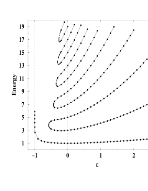
FIG. 1.: Energy levels of the Hamiltonian $H=p^{2}+x^{2}(ix)^{\epsilon}$ as functions of the parameter $\epsilon$. There are three regions: When $\epsilon\geq 0$ the spectrum is entirely real and positive. All eigenvalues rise monotonically with increasing $\epsilon$. The lower bound of this region, $\epsilon=0$, corresponds to the harmonic oscillator, whose energy levels are $E_{k}=2k+1$. When $-1<\epsilon<0$, there are a finite number of real positive eigenvalues and an infinite number of complex conjugate pairs of eigenvalues. As $\epsilon$ decreases from $0$ to $-1$, the number of real eigenvalues decreases. As $\epsilon$ approaches $-1^{+}$, the ground-state energy diverges. For $\epsilon\leq-1$ there are no real eigenvalues.

In the past we have always regarded the parameter $\epsilon$ as being small; we have defined theories by analytically continuing away from $\epsilon=0$. However, in this paper we investigate the large-$\epsilon$ limit of the Hamiltonian in Eq. (4). We will show that in this limit the theory becomes exactly solvable. An exact formula for the $k$th energy level in the limit of large $\epsilon$ is

$$E_{k}(\epsilon)\sim{1\over 4}\left(k+{1\over 2}\right)^{2}\epsilon^{2}\qquad(\epsilon\to\infty).$$ (5)

More generally, we will consider the large-$\epsilon$ limit of an infinite number of classes of ${\cal PT}$-symmetric Hamiltonians of the form [3]

$$H=p^{2}+x^{2M}(ix)^{\epsilon}\qquad(\epsilon\geq 0,~{}M=1,2,3,\ldots).$$ (6)

For each positive integer value of $M$, these Hamiltonians may be regarded as complex deformations of the Hermitian Hamiltonian $H=p^{2}+x^{2M}$ in Eq. (3). In the limit as $\epsilon\to\infty$ each of these Hamiltonians becomes exactly solvable; the spectrum for large $\epsilon$ is given by

$$E_{k}(M,\epsilon)\sim{1\over 4}\left(k+{P\over M+1}\right)^{2}\epsilon^{2}\qquad(\epsilon\to\infty),$$ (7)

where $P=1,2,3,\ldots,M$.

For the Hamiltonian $H$ in Eq. (6) the Schrödinger differential equation corresponding to the eigenvalue problem $H\psi=E\psi$ is

$$-\psi^{\prime\prime}(x)+x^{2M}(ix)^{\epsilon}\psi(x)=E\psi(x).$$ (8)

To obtain real eigenvalues from this equation it is necessary to define the boundary conditions properly. The regions in the cut complex-$x$ plane in which $\psi(x)$ vanishes exponentially as $|x|\to\infty$ are wedges. In Refs. [2, 3] the wedges for $\epsilon>0$ were chosen to be the analytic continuations of the wedges for the anharmonic oscillator ($\epsilon=0$), which are centered about the negative and positive real axes and have angular opening $\pi/(M+1)$. This analytic continuation defines the boundary conditions in the complex-$x$ plane. For arbitrary $\epsilon>0$ the anti-Stokes’ lines at the centers of the left and right wedges lie below the real axis at the angles

$$\theta_{\rm left} = -\pi+{\epsilon\pi\over 4M+2\epsilon+4},$$ (9)

$$\theta_{\rm right} = -{\epsilon\pi\over 4M+2\epsilon+4}.$$ (11)

The opening angle of each of these wedges is $2\pi/(2M+\epsilon+2)$. In Refs. [2, 3] the time-independent Schrödinger equation was integrated numerically inside the wedges to determine the eigenvalues to high precision. Observe that as $\epsilon$ increases from its anharmonic oscillator value ($\epsilon=0$), the wedges bounding the integration path undergo a continuous deformation as a function of $\epsilon$. As $\epsilon$ increases, the opening angles of the wedges become smaller and both wedges rotate downward towards the negative-imaginary axis. Also, note that the angular difference $\theta_{\rm right}-\theta_{\rm left}=2\pi(M+1)/\epsilon$ approaches zero as $\epsilon$ increases.

This paper is organized very simply. In Sec. II we consider the special case $M=1$ in Eq. (4). Then in Sec. III we generalize to the case of arbitrary integer $M$ in Eq. (6). Finally, in Sec. IV we examine expansions about the $\epsilon\to\infty$ limit of the theory.

II Special Case $M=1$.

The eigenvalues of $H$ in Eq. (4) can be found approximately using WKB theory. The left and right turning points for this calculation lie inside the left and right wedges at

$$x_{\rm left} = E^{1/(2+\epsilon)}\exp\left(-i\pi+{\epsilon\over 2\epsilon+4}i\pi\right),$$ (12)

$$x_{\rm right} = E^{1/(2+\epsilon)}\exp\left(-{\epsilon\over 2\epsilon+4}i\pi\right).$$ (13)

As explained in Ref. [2], the WKB quantization formula is

$$\left(k+{1\over 2}\right)\pi\sim\int_{x_{\rm left}}^{x_{\rm right}}dx\,\sqrt{E-x^{2}(ix)^{\epsilon}}\quad(k\to\infty),$$ (14)

where the path of integration is a curve from the left turning point to the right turning point along which the quantity $dx$ times the integrand of Eq. (14) is real. This path lies in the lower-half $x$ plane and is symmetric with respect to the imaginary axis. The path resembles an inverted parabola; it emerges from the left turning point and rises monotonically until it crosses the imaginary axis; it then falls monotonically until it reaches the right turning point. As calculated in Ref. [2], the WKB quantization formula (14) gives

$$E_{k}\sim\left[{\Gamma\left({3\epsilon+8\over 2\epsilon+4}\right)\sqrt{\pi}\left(k+{1\over 2}\right)\over\sin\left({\pi\over\epsilon+2}\right)\Gamma\left({\epsilon+3\over\epsilon+2}\right)}\right]^{2\epsilon+4\over\epsilon+4}\quad(k\to\infty).$$ (15)

When the parameter $\epsilon$ is large, the right side of Eq. (15) simplifies dramatically and we have the result in Eq. (5) with corrections of order $\epsilon\ln\epsilon$. As we will see, this happens to be the exact answer for all energy levels; that is, for all values of $k$. Since the WKB formula in Eq. (15) is only valid for large $k$ with $\epsilon$ fixed, it is not at all obvious why the leading-order WKB calculation gives the exact answer.

It is surprising to learn that the energy levels grow as $\epsilon^{2}$ for large $\epsilon$. Recall that the energy levels of the Hamiltonian in Eq. (3) approach finite limits as $M\to\infty$. [These limits are the energy levels of the conventional square well $V_{\rm SW}$ in Eq. (1).] To understand why the energy levels for the ${\cal PT}$-symmetric Hamiltonian in Eq. (4) grow as $\epsilon^{2}$ we use the uncertainty principle. From Eq. (13) we see that the turning points rotate towards each other as $\epsilon\to\infty$. (They both approach the point $-i$ on the negative imaginary axis.) Indeed, the distance between the turning points is of order $1/\epsilon$. [For the case of the Hamiltonian $H$ in Eq. (3) the turning points stabilize at $\pm 1$ as $M\to\infty$.] Thus, the quantum particle is trapped in a region whose size $\Delta x$ is of order $1/\epsilon$. The uncertainty in the momentum $\Delta p$ of the particle is therefore of order $\epsilon$. Finally, since the energy is the square of the momentum, we conclude that the energy levels must be of order $\epsilon^{2}$.

Let us rederive this result using the time-energy version of the uncertainty principle. As explained in Refs. [2, 3], a classical particle described by the Hamiltonian in Eq. (4) exhibits periodic motion. The period $T$ of this complex pendulum is given exactly by the formula

$$T=4\sqrt{\pi}E^{-{\epsilon\over 4+2\epsilon}}{\Gamma\left({3+\epsilon\over 2+\epsilon}\right)\cos\left({\epsilon\pi\over 4+2\epsilon}\right)\over\Gamma\left({4+\epsilon\over 4+2\epsilon}\right)}.$$ (16)

For large $\epsilon$ we have

$$T\sim 4\pi/(\epsilon\sqrt{E})\qquad(\epsilon\to\infty).$$ (17)

Multiplying this equation by $E$ gives the product $ET$ on the left side, which, by the uncertainty principle is of order 1. Thus, solving for $E$, we find again that $E$ is of order $\epsilon^{2}$ for large $\epsilon$.

This last calculation illustrates an important difference between conventional quantum theories and ${\cal PT}$-symmetric quantum theories. In a conventional Hermitian theory both the classical periodic motion and the WKB path of integration coincide; this classically allowed region lies on the real axis between the turning points. For ${\cal PT}$-symmetric theories the WKB contour and the classical path do not coincide. The classical periodic motion follows a path joining the turning points that, like the WKB path, is symmetric about the negative imaginary axis. However, unlike the WKB path, the classical path moves downward rather than upward as it approaches the negative-imaginary axis (see, for example, Fig. 2 of Ref. [3]).

Having discussed this problem heuristically, we now give a precise calculation of the spectrum in the limit of large $\epsilon$. We begin by substituting

$$x=\left(-i+{z\pi\over 2+\epsilon}\right)E^{1\over 2+\epsilon}$$ (18)

into Eq. (8) with $M=1$. The resulting differential equation for large $\epsilon$ is

$${d^{2}\over dz^{2}}\psi(z)+F\pi^{2}\left(1+e^{iz\pi}\right)\psi(z)=0,$$ (19)

where

$$F=E/\epsilon^{2}$$ (20)

and we have used the identity $\lim_{\epsilon\to\infty}(1+x/\epsilon)^{\epsilon}=e^{x}$.

The advantage of the differential equation (19) is that it is independent of $\epsilon$. [As such, this equation corresponds to the $M$-independent Schrödinger equation for the square well that is obtained from Eq. (3) in the limit of large $M$.] In the variable $z$ the turning points at $z=-1$ and $z=1$ are fixed and well separated in the limit of large $\epsilon$. The large-$\epsilon$ behavior of $E$ in Eq. (5) is already evident in Eq. (20). Imposing the appropriate boundary conditions on Eq. (19) gives eigenvalues $F$ that are clearly independent of $\epsilon$. Thus, for large $\epsilon$ we see that $E$ grows like $\epsilon^{2}$.

Because there is no longer any small parameter in Eq. (19), this equation cannot be solved approximately using a perturbative method such as WKB. It is necessary to solve this equation exactly. Fortunately, we can solve it exactly by making a simple substitution. The change of variable

$$w=2\sqrt{F}e^{i\pi z/2}$$ (21)

converts Eq. (19) to a modified Bessel equation [4]:

$$w^{2}{d^{2}\over dw^{2}}\psi(w)+w{d\over dw}\psi(w)-\left(w^{2}+\nu^{2}\right)\psi(w)=0,$$ (22)

where

$$\nu=2\sqrt{F}.$$ (23)

The exact solution to this equation is a linear combination of modified Bessel functions [4]:

$$\psi(w)=C_{1}I_{\nu}(w)+C_{2}K_{\nu}(w),$$ (24)

where $C_{1}$ and $C_{2}$ are arbitrary constants. Thus, in terms of the $z$ variable we have

$$\psi(z)=C_{1}I_{\nu}\left(\nu e^{i\pi z/2}\right)+C_{2}K_{\nu}\left(\nu e^{i\pi z/2}\right).$$ (25)

We must now impose boundary conditions on $\psi(z)$. Emanating from the turning points at $z=-1$ and $z=1$ are three Stokes’ lines (lines along which the solution is purely oscillatory and not growing or falling exponentially) and three anti-Stokes’ lines (lines along which the solution is purely exponential and not oscillatory). These Stokes’ and anti-Stokes’ lines are shown as dashed and solid lines on Fig. 2. The Stokes’ lines emerge from the turning points going up to the left and the right at $30^{\circ}$ and also directly down. The anti-Stokes’ lines emerge from the turning points going down to the left and the right at $30^{\circ}$ and directly up. Note that the Stokes’ line going up to the right from the turning point at $z=-1$ joins continuously onto the Stokes’ line going up to the left from the turning point at $z=1$. The anti-Stokes’ lines going down to the left from $z=-1$ and down to the right from $z=1$ eventually become vertical and asymptote to the lines ${\rm Re}\,z=-2$ and ${\rm Re}\,z=2$. We impose the boundary conditions that $\psi(z)\to 0$ on these anti-Stokes’ lines because these correspond to the center lines of the wedges in Eq. (11) in the complex-$x$ plane (for $M=1$).

To summarize, in the large-$\epsilon$ limit of the Hamiltonian in Eq. (4), the eigenvalue problem for the scaled eigenvalues $F$ is a two-turning-point problem that lies along an arch-shaped contour. The legs of the arches lie below the real-$z$ axis and approach $\pm 2-i\infty$. The turning points at $z=\pm 1$ are joined by the Stokes’ line lying above the real-$z$ axis as indicated in Fig. 2. This is the complex version of the infinite-square-well problem in elementary quantum mechanics. In the square-well problem there are also two turning points at $\pm 1$ joined by a Stokes’ line lying on the real axis. However, there are no anti-Stokes’ lines along which the wave function dies away exponentially; the wave function simply vanishes at the turning points.

The quantized energy levels are determined by imposing the boundary conditions discussed above on the modified Bessel functions in Eq. (25). For simplicity, we impose these conditions on the vertical lines $z=\pm 2-iy$, where $y\to+\infty$. In terms of the variable $y$ the wave function $\psi$ in Eq. (25) becomes

$$\psi(y)=C_{1}I_{\nu}\left(\nu e^{-i\pi}e^{\pi y/2}\right)+C_{2}K_{\nu}\left(\nu e^{-i\pi}e^{\pi y/2}\right)$$ (26)

at $z=-2-iy$, and

$$\psi(y)=C_{1}I_{\nu}\left(\nu e^{i\pi}e^{\pi y/2}\right)+C_{2}K_{\nu}\left(\nu e^{i\pi}e^{\pi y/2}\right)$$ (27)

at $z=2-iy$.

FIG. 2.: Stokes’ lines and anti-Stokes’ lines for the differential equation (19). Three Stokes’ lines (dashed lines) and three anti-Stokes’ lines (solid lines) emerge from the turning points at $z=\pm 1$. The path of integration for the WKB quantization condition in Eq. (14) corresponds to the arch-shaped dotted line connecting the turning points.

Our objective now is to simplify these equations by making the arguments of the modified Bessel equations entirely real and positive. To do so we use the following functional equations satisfied by $I_{\nu}$ and $K_{\nu}$ [4]:

$$I_{\nu}\left(e^{m\pi i}z\right) = e^{m\nu\pi i}I_{\nu}(z),$$ (28)

$$K_{\nu}\left(e^{m\pi i}z\right) = e^{-m\nu\pi i}K_{\nu}(z)-i\pi{\sin(m\nu\pi)\over\sin(\nu\pi)}I_{\nu}(z),$$ (29)

where $m$ is an integer. According to these relations, Eq. (26) becomes

$$\psi(y) = C_{1}e^{-\nu\pi i}I_{\nu}\left(\nu e^{\pi y/2}\right)$$ (30)

$$+ C_{2}\left[e^{\nu\pi i}K_{\nu}\left(\nu e^{\pi y/2}\right)+i\pi I_{\nu}\left(\nu e^{\pi y/2}\right)\right]$$ (31)

and Eq. (27) becomes

$$\psi(y) = C_{1}e^{\nu\pi i}I_{\nu}\left(\nu e^{\pi y/2}\right)$$ (32)

$$+ C_{2}\left[e^{-\nu\pi i}K_{\nu}\left(\nu e^{\pi y/2}\right)-i\pi I_{\nu}\left(\nu e^{\pi y/2}\right)\right].$$ (33)

Next, we use the asymptotic behavior of the modified Bessel functions for large positive argument. The function $I_{\nu}(r)$ grows exponentially and the function $K_{\nu}(r)$ decays exponentially for large positive $r$ [4]:

$$I_{\nu}(r) \sim {1\over\sqrt{2\pi r}}\,e^{r}\qquad(r\to+\infty),$$ (34)

$$K_{\nu}(r) \sim \sqrt{\pi\over 2r}\,e^{-r}\qquad(r\to+\infty).$$ (35)

Eliminating the growing exponentials in Eqs. (31) and (33) gives a pair of linear equations to be satisfied by the coefficients $C_{1}$ and $C_{2}$:

$$C_{1}e^{-\nu\pi i}+C_{2}i\pi = 0,$$ (36)

$$C_{1}e^{\nu\pi i}-C_{2}i\pi = 0.$$ (37)

A nontrivial solution to Eq. (37) exists only if the determinant of the coefficients vanishes:

$${\rm det}\left(\begin{array}[]{cc}e^{-\nu\pi i}&i\pi\\ e^{\nu\pi i}&-i\pi\end{array}\right)=-2i\pi\cos(\nu\pi)=0.$$ (40)

TABLE I.: Comparison of the numerical values of $F(\epsilon)$ with that predicted in Eq. (41) for the ground state $k=0$ of an $x^{2}(ix)^{\epsilon}$ theory. The second column gives the exact values of the ground-state energy for various values of $\epsilon$ in the first column. In the third column is the value of $F$ obtained from the exact energy in the second column using Eq. (51), which is a more precise version of Eq. (20). Finally, in the fourth and fifth columns are the first and second Richardson extrapolants [5] of the numbers in the third column. Note that the exact values of $F(\epsilon)$ and their Richardson extrapolants rapidly approach the asymptotic value $1/16=0.0625.$

$\epsilon$	$E_{0}(\epsilon)$	$F(\epsilon)$	$R_{1}(\epsilon)$	$R_{2}(\epsilon)$
8	$5.55331$	$0.07825$	$-$	$-$
18	$20.67629$	$0.06998$	$0.06336$	$-$
28	$46.94324$	$0.06742$	$0.06281$	$0.06259$
38	$84.78728$	$0.06617$	$0.06266$	$0.06253$
48	$134.43752$	$0.06542$	$0.06260$	$0.06251$
58	$196.03417$	$0.06493$	$0.06257$	$0.06251$

Hence, $\nu=k+{1\over 2}$, and from Eq. (23), we have the exact result

$$F={1\over 4}\left(k+{1\over 2}\right)^{2}\qquad(k=0,1,2,3,\ldots).$$ (41)

Finally, we use Eq. (20) to obtain the large-$\epsilon$ behavior of the eigenvalues $E$ given in Eq. (5). We verify this result numerically in Table I.

III Arbitrary Integer $M$

The calculation of the energy levels for the general class of theories given in Eq. (6) is a straightforward generalization of the calculation for the case $M=1$ in Sec. II. The crucial ingredient in the calculation is understanding the array of Stokes’ and anti-Stokes’ lines along which we impose the boundary conditions. This difference leads to $M$-dependent wave functions, but the condition that determines the eigenvalues is still a simple trigonometric equation.

Just as for the case $M=1$, we scale the differential equation (8) using Eq. (18). In the limit as $\epsilon\to\infty$ the resulting differential equation is identical to Eq. (19) except that now there is a factor of $(-1)^{M+1}$ multiplying the exponential term. Again, we define $F$ as in Eq. (20) and change to the variable $w$ as prescribed by Eq. (21). This gives the differential equation

$$w^{2}{d^{2}\over dw^{2}}\psi(w)+w{d\over dw}\psi(w)$$ (42)

$$\qquad-\left[(-1)^{M+1}w^{2}+\nu^{2}\right]\psi(w)=0,$$ (43)

which is the generalization of Eq. (22). In this equation $\nu$ is defined as before by Eq. (23). Note that except for the appearance of the $(-1)^{M+1}$ multiplying the $w^{2}$ term this equation is independent of $M$.

To solve Eq. (43) we consider the two cases of odd $M$ and even $M$ separately. If $M$ is odd this equation is identical to Eq. (22), and the general solution is that given in Eq. (24). If $M$ is even Eq. (43) is no longer a modified Bessel equation, but instead is just the standard Bessel equation. Hence, in this case the general solution to Eq. (43) is a linear combination of the ordinary Bessel functions $J_{\nu}$ and $Y_{\nu}$:

$$\psi(w)=C_{1}J_{\nu}(w)+C_{2}Y_{\nu}(w).$$ (44)

Thus, in terms of the variable $z$ the wave function in this case is

$$\psi(z)=C_{1}J_{\nu}\left(\nu e^{i\pi z/2}\right)+C_{2}Y_{\nu}\left(\nu e^{i\pi z/2}\right).$$ (45)

Although it appears that this solution is independent of the parameter $M$, one must recall that the boundary conditions do depend on $M$. Thus, the wave functions and energy eigenvalues do indeed depend on $M$. To be precise, for a given $M$ the Stokes’ lines emanating from $z=\pm M$ are joined by a string of adjacent arches of length $2$. The anti-Stokes’ lines leave $\pm M$ and asymptote to the lines ${\rm Re}\,z=\pm(M+1)$.

For odd $M$ we impose the boundary conditions as for the case $M=1$ except that the wave function $\psi$ vanishes along different lines. For even $M$ the wave functions in Eq. (45) must first be expressed in terms of modified Bessel functions using the functional equations [4]

$$J_{\nu}(iz) = e^{\nu\pi i/2}I_{\nu}(z),$$ (46)

$$Y_{\nu}(iz) = {-2\over\pi}e^{-\nu\pi i/2}K_{\nu}(z)+ie^{\nu\pi i/2}I_{\nu}(z),$$ (47)

and then be treated using the same procedure as for odd $M$.

Although the matrix elements for the linear equations obtained for odd $M$ and even $M$ are quite different, the eigenvalue conditions are similar. For $M=2$ the condition is

$$\cos(2\nu\pi)=-1/2,$$ (48)

whose solution is

$$\nu=k+{1\over 3}\quad{\rm and}\quad\nu=k+{2\over 3}.$$ (49)

Thus, for large $\epsilon$ the energy is given by

$$E={1\over 4}\left(k+{P\over 3}\right)^{2}\epsilon^{2},$$ (50)

where $P=1,2$. Note that this result is the $M=2$ case of Eq. (7). This expression is verified numerically in Table II for the case of the ground state energy corresponding to $k=0$ and $P=1$. For arbitrary $M$ one obtains the result in Eq. (7).

TABLE II.: Comparison of the numerical values of $F(\epsilon)$ with that predicted in Eq. (50) for the ground state $k=0,P=1$ of an $x^{4}(ix)^{\epsilon}$ theory. The second column gives the exact values of the ground-state energy for various values of $\epsilon$ in the first column. In the third column is the value of $F$ obtained from the energy in the second column using Eq. (51). Finally, in the fourth and fifth columns are the first and second Richardson extrapolants [5] of the numbers in the third column. Note that the exact values of $F(\epsilon)$ and their Richardson extrapolants rapidly approach the asymptotic value $1/36=0.0277778.$

$\epsilon$	$E_{0}(\epsilon)$	$F(\epsilon)$	$R_{1}(\epsilon)$	$R_{2}(\epsilon)$
8	$2.65128$	$0.05035$	$-$	$-$
18	$9.21477$	$0.03551$	$0.02661$	$-$
28	$20.70525$	$0.03232$	$0.02722$	$0.02740$
38	$37.32010$	$0.03097$	$0.02746$	$0.02766$
48	$59.16865$	$0.03023$	$0.02756$	$0.02772$
58	$86.31766$	$0.02977$	$0.02764$	$0.02775$

Observe that the magnitude of the energy eigenvalues decreases as $M$ increases. At first glance this might seem surprising, but it can be easily understood in terms of the uncertainty principle. As $M$ increases, the anti-Stokes’ lines on which we impose the boundary conditions for the differential equation (8) move away from the negative imaginary axis, as we can see from Eq. (11). For example, for fixed $\epsilon$ the anti-Stokes’ lines for $M=2$ are separated by a greater distance than for $M=1$; the anti-Stoke’s lines for $M=3$ are separated by a greater distance than for $M=2$, and so on. Hence, the uncertainty in the position $\Delta x$ increases with $M$. By the uncertainty principle, this increase in the uncertainty of the position corresponds to a decrease in the uncertainty of the momentum, and thus, a decrease in the energy. This argument explains the large-$M$ behavior of the result in Eq. (7).

IV Higher-Order Corrections to the $\epsilon\to\infty$ Limit for $M=1$

In this section we show how to calculate the corrections to the large-$\epsilon$ behavior in Eq. (5). These corrections are of order $\epsilon$ and $\epsilon\ln\epsilon$. From these higher-order calculations we obtain an extremely accurate approximation $E_{k}$ for all $k$. Our asymptotic analysis begins with the change of variable in Eq. (18), but we use a more precise version of Eq. (20):

$$F(\epsilon)={E^{\epsilon+4\over\epsilon+2}\over(\epsilon+2)^{2}}.$$ (51)

We find that the function $F(\epsilon)$ is a series in inverse powers of $\epsilon$ of the form $F=f_{0}+f_{1}\epsilon^{-1}+f_{2}\epsilon^{-2}+\cdots$. The coefficient $f_{0}=F(\infty)$ is given in Eq. (41). Our objective here is to calculate $f_{1}$, and from this to calculate the first correction to $E$.

In addition to $F(\epsilon)$, the wave function $\psi$ is also a series in inverse powers of $\epsilon$, $\psi(z)=\psi_{0}+\psi_{1}(z)\epsilon^{-1}+\psi_{2}(z)\epsilon^{-2}+\cdots$. Using this series and collecting like powers of $\epsilon$ we obtain the following sequence of differential equations:

$$\epsilon^{0}:\quad{d^{2}\over dz^{2}}\psi_{0}(z)+f_{0}\pi^{2}\left(1+e^{iz\pi}\right)\psi_{0}(z)=0,$$ (52)

$$\epsilon^{-1}:\quad{d^{2}\over dz^{2}}\psi_{1}(z)+f_{0}\pi^{2}\left(1+e^{iz\pi}\right)\psi_{1}(z)$$ (53)

$$\qquad\qquad=-\left[f_{0}\pi^{2}e^{iz\pi}{z^{2}\over 2}+f_{1}(1+e^{iz\pi})\right]\pi^{2}\psi_{0}(z),$$ (54)

$$\epsilon^{-2}:\quad{d^{2}\over dz^{2}}\psi_{2}(z)+f_{0}\pi^{2}\left(1+e^{iz\pi}\right)\psi_{2}(z)$$ (55)

$$\qquad\qquad=-\left[f_{0}\pi^{2}e^{iz\pi}{z^{2}\over 2}+f_{1}(1+e^{iz\pi})\right]\pi^{2}\psi_{1}(z)$$ (56)

$$\qquad\qquad-\left[f_{0}e^{iz\pi}\left(z^{2}\pi^{2}+z^{3}\pi^{3}i-{z^{4}\pi^{4}\over 8}\right)\right.$$ (57)

$$\qquad\qquad\left.+f_{1}e^{iz\pi}{z^{2}\pi^{2}\over 2}+f_{2}\left(1+e^{iz\pi}\right)\right]\pi^{2}\psi_{0}(z).$$ (58)

The first equation is exactly Eq. (19). The second equation contains the coefficient $f_{1}$. To solve for $f_{1}$ we observe that the solution to the homogeneous part of the equation is just the solution to the first equation. This suggests using the method of reduction of order; to wit, we let $\psi_{1}(z)=u_{1}(z)\psi_{0}(z)$. To solve the resulting equation for $f_{1}$ we then multiply by $\psi_{0}(z)$ and integrate over the $WKB$ path with respect to $z$. The first equation can be used to simplify this equation and the left side becomes the expression $u_{1}(z)\psi_{0}^{2}(z)$ evaluated at the end points. Since $\psi_{0}(-i\infty)=0$, the left side equals zero, and we can solve for $f_{1}$ in quadrature form. To be explicit,

$$f_{1}=-{1\over 2}f_{0}\pi^{2}{\int_{-2-i\infty}^{2-i\infty}dz\,z^{2}\psi_{0}^{2}(z)e^{iz\pi}\over\int_{-2-i\infty}^{2-i\infty}dz\,\psi_{0}^{2}(z)(1+e^{iz\pi})}.$$ (59)

To prepare for evaluating these integrals we change to the variable $w$ in Eq. (21) with $F=f_{0}$ and obtain

$$f_{1}={1\over 2}{\int_{-\infty+i\delta}^{-\infty-i\delta}dw\,w\psi_{0}^{2}(w)\ln^{2}\left({w\over 2\sqrt{f_{0}}}\right)\over\int_{-\infty+i\delta}^{-\infty-i\delta}{dw\over w}\psi_{0}^{2}(w)\left(1+{w^{2}\over 4f_{0}}\right)},$$ (60)

where $\delta$ is infinitesimal and the contour of integration goes around the origin.

For the case $k=0$ these integrals are easy to evaluate because $f_{0}=1/16$ and $\psi_{0}(w)=I_{1/2}(w)+K_{1/2}(w)/\pi=e^{w}/\sqrt{2\pi w}$. Substituting these expressions into Eq. (60) gives

$$f_{1}={1\over 2}{\int_{-\infty+i\delta}^{-\infty-i\delta}dw\,e^{2w}\ln^{2}(2w)\over\int_{-\infty+i\delta}^{-\infty-i\delta}dw\,e^{2w}\left(4+{1\over w^{2}}\right)}.$$ (61)

By carefully evaluating the discontinuities across the branch cut and the residues at the singularities of the integrands, we obtain

$$f_{1}=\gamma/4,$$ (62)

where $\gamma$ is Euler’s constant. Combining this result with Eq. (51) and solving for $E$ in the limit of large $\epsilon$ yields

$$E={1\over 16}\epsilon^{2}-{1\over 4}\epsilon\ln\epsilon+{1\over 4}(1+\gamma+2\ln 2)\epsilon+{\rm O}(\ln\epsilon).$$ (63)

By comparison, if we calculate to next order in WKB, we obtain for the $k$th energy level

$$E_{k} \sim \left[{\Gamma\left({8+3\epsilon\over 4+2\epsilon}\right)\sqrt{\pi}(k+1/2)\over\sin\left({\pi\over 2+\epsilon}\right)\Gamma\left({3+\epsilon\over 2+\epsilon}\right)}\right]^{4+2\epsilon\over 4+\epsilon}$$ (64)

$$\times \left[1+{(2+\epsilon)(1+\epsilon)\sin\left({2\pi\over 2+\epsilon}\right)\over 6\pi(k+1/2)^{2}(4+\epsilon)^{2}}\right]\quad(k\to\infty).$$ (65)

Taking the large $\epsilon$ limit of this expression gives

$$E={\epsilon^{2}\over 16}-{1\over 4}\epsilon\ln\epsilon+{1\over 4}\left({7\over 3}+\ln 2\right)\epsilon+{\rm O}(\ln\epsilon).$$ (66)

The appearance of a $\log\epsilon$ term in this behavior is a consequence of the structure of Eq. (51). Note that the coefficent of the $\epsilon$ term for $WKB$ differs from the exact result but $WKB$ is numerically very accurate. WKB gives $0.75662$ compared with $0.74088$ for the exact result.

In Table III the results of a Richardson extrapolation [5] of the exact values of $F(\epsilon)$ are given. These results verify that the value of $f_{1}$ is correct.

This work was supported in part by the U.S. Department of Energy.

TABLE III.: Comparison of the numerical value of the coefficient $f_{1}$ in Eq. (62) with a fit to the exact values of $F(\epsilon)$ for the case of the ground state $k=0$ of an $x^{2}(ix)^{\epsilon}$ theory. The second column gives the exact values of the ground-state energy for various values of $\epsilon$ in the first column. In the third column is the approximation to $f_{1}$ obtained from $F(\epsilon)$ by subtracting off the leading large-$\epsilon$ behavior given in Eq. (41). In the fourth and fifth columns are the first and second Richardson extrapolants [5] of the numbers in the third column. Note that the approximations in column 3 and their Richardson extrapolants rapidly approach the asymptotic value of $f_{1}=\gamma/4=0.144304$.

$\epsilon$	$E_{0}(\epsilon)$	$R_{0}(\epsilon)$	$R_{1}(\epsilon)$	$R_{2}(\epsilon)$
8	$5.55331$	$0.12597$	$-$	$-$
18	$20.67629$	$0.13460$	$0.14150$	$-$
28	$46.94324$	$0.13767$	$0.14321$	$0.14389$
38	$84.78728$	$0.13926$	$0.14372$	$0.14418$
48	$134.43752$	$0.14024$	$0.14394$	$0.14425$
58	$196.03417$	$0.14090$	$0.14406$	$0.14428$

REFERENCES

[1] S. Boettcher and C. M. Bender, J. Math. Phys. 31, 2579
(1990).
[2] C. M. Bender and S. Boettcher, Phys. Rev. Lett. 80, 5243
(1998).
[3] See C. M. Bender, S. Boettcher, and
P. N. Meisinger, J. Math. Phys. 40, 2201 (1999).
[4] M. Abramowitz and I. A. Stegun, Handbook of Mathematical
Functions (National Bureau of Standards, Washington, 1964), chap. 9.
[5] C. M. Bender and S. A. Orszag, Advanced Mathematical
Methods for Scientists and Engineers (McGraw-Hill, New York, 1978), Chap. 8.