The Best Copenhagen Tunneling Times

Abstract

Recently, people have caculated tunneling’s characteristic times within Bohmian mechanics. Contrary to some characteristic times defined within the framework of the standard interpretation of quantum mechanics, these have reasonable values. Here, we introduce one of available definitions for tunnelling’s characteristic times within the standard interpretation as the best definition that can be accepted for the tunneling times. We show that, due to experimental limitations, Bohmian mechanics leads to same tunneling times.

I Introduction

A problem which does not have a clear cut answer in quantum mechanics, is the time that it takes for an electron to pass through a potential barrier. This is a problem that is important from both a theoretical perspective[1, 2] and a technological view[3, 4].

In quantum mechanics, time enters as a parameter rather than an observable (to which an operator can be assigned). Thus, there is no direct way to calculate tunneling times. People have tried to introduce quantities which have the dimension of time and can somehow be associated with the passage of the particle through the barrier. These efforts have led to the introduction of several times, some of which are completely unrelated to the others [5-17]. Some people have used Larmor precession as a clock[5] to measure the duration of tunneling for a steady state [6, 7] or for a wave packet[8]. Others, have used Feynman paths like real paths to calculate an average tunneling time with the weighting function $exp[iS(x(t))/\hbar]$, where $S$ is the action associated with the path $x(t)$- where $x(t)$’s are Feynman paths initiated from a point on the left of the barrier and ending at another point on the right of it[9]. On the other hand, a group of people have used some features of an incident wave packet and the comparable features of the transmitted packet to introduce a delay as tunneling time[10, 18]. There are many other approaches, some of which are mentioned in Refs. [10-17]. But, there is no general consensus among physicists about the meaning of them and about which, if any, of them being the proper tunneling time. In Bohmian mechanics[19], however, there is a unique way of identifying the time of passage through a barrier. This time has a reasonable behaviour with respect to the width of the barrier and the energy of particle[20, 21].

It is expected that with the availability of reliable experimental results in the near future, an appropriate definition can be selected from the available ones, or that they would prepare the ground for a more appropriate definition of the transmission time. But now, we want to use the definition of tunneling time in the framework of Bohmian mechanics to select one of available definitions for quantum tunneling times (QTT) within the standard interpretation as the best definition.

Our paper is organized as follows: after introducing Olkhovsky-Recami QTT, by using a heuristic argument in section II, we introduce, in section III, Bohmian QTT. Then, in section IV, we give a critical discussion about Cushing’s thought experiment and about what it really measures.

II Tunneling’s characteristic times in the Copenhagen framework

To begin with, we consider the time at which a particle passes through a definite point in space. We describe the particle by a Gaussian wave packet which is incident from the left. The most natural way to estimate this time of passage is to find the time at which the peak of the wave packet passes through that point. But this is not a right criterion for finding the time of passage of the particle (even if the wave packet is symmetrical). To clarify the matter, we divide the packet, in the middle, into two parts. The probability of finding the particle in the front section is $\frac{1}{2}$ and the same is true for the back section. We represent the transit time of the centre of gravity of the front section by $t_{1}$ and that of the back section by $t_{2}$. The average time for particle’s passage through that point is $T=\frac{1}{2}(t_{1}+t_{2})$. If the transit time for the peak of the wave is denoted by $t$, we have:

$$t_{1}=t-\frac{x_{1}}{v_{g}}$$ (2)

$$t_{2}=t+\frac{x_{2}}{v_{g}}$$ (3)

where $v_{g}$ is the group velocity of the wave packet and $x_{1}$ and $x_{2}$ are, respectively, the distances of the centers of gravity of the front and the back sections of the packet from its peak position, when these centers pass the point under consideration. Thus, we have:

$$T=\frac{1}{2}(t_{1}+t_{2})=t+\frac{x_{2}-x_{1}}{2v_{g}}$$ (4)

If the wave packet did not spread, $x_{1}$ and $x_{2}$ would remain equal and $T$ would be equal to $t$. But, since the wave packet spreads, $T\neq t$. In fact, the average transit time for the particle is later than that of wave’s peak. Because, the spreading of the packet decreases the transit time of the centre of gravity of wave’s front section, and increases that of the back

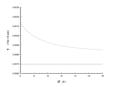
FIG. 1.: Average time for the transmission of the probability flux ($---$) and the passage of the peak (——), for packets having different widths ($\sigma$).

section. But the change is not symmetrical (i.e. $x_{1}\neq x_{2}$), as the back section of the wave experiences the spreading for a longer time.

Now, consider a wave packet $\psi(x,t)$, which is incident from the left and approaches a far point $x$. The best time that we can attribute to particle’s passage through $x$ is

$$\tau(x)=\frac{\int_{0}^{\infty}t\ |\psi(x,t)|^{2}\ v(x,t)\ dt}{\int_{0}^{\infty}\ |\psi(x,t)|^{2}\ v(x,t)\ dt}$$ (5)

where $v(x,t)=$$\frac{j(x,t)}{|\psi(x,t)|^{2}}$, $j(x,t)$ being the probability current density. In fact, we have divided the wave packet into infinitesimal elements. The transit time when particle is in one of these elements is weighted by the probability of finding the particle there (i.e. $|\psi(x,t)|^{2}\ dx=|\psi(x,t)|^{2}\ v(x,t)\ dt$). Fig.(1) illustrates the difference between this time and the time that the peak passes that point. For narrow wave packets, for which the rate of spreading is large, this difference is large. From (3), one can define a distribution for the transit time through $x$:

$$P(x,t)=\frac{|\psi(x,t)|^{2}\ v(x,t)}{\int_{0}^{\infty}|\psi(x,t)|^{2}\ v(x,t)dt}=\frac{j(x,t)}{|T|^{2}}$$ (6)

where $|T|^{2}$ is the transition probability for passing through $x_{o}$. Dumont and Marchioro introduced this definition for the distribution of the time at which a particle passes through the far side of a potential barrier[22]. They did not find it possible to define the time spent by the particle in the barrier. Leavens showed that this is also the distribution for the same time in Bohmian mechanics[23].

By looking at (3), one notices that $\tau(x)$ is in fact the average time for the passage of the probability density $|\psi|^{2}$ through $x_{o}$. Since the probability density represents the probability of the presence of the particle, it is natural to take the average time for the passage of probability density through a point as a measure of the average time for particle’s passage through that point. But, while part of the probability flux passes through the barrier, the particle itself might not be detected on the other side of the barrier. We don’t, however, expect to get a definite prediction for an individual system, and in the laboratory we usually consider an ensemble of systems. Thus, it is natural to take the average time for the passage of the probability density as a measure of the average time for particle’s passage. From now on, we talk about particle’s average time of transit. Consider, a particle incident on a barrier from the left. Then, one can easily extend (3) to define average times for particle’s entrance into the barrier ($\tau_{{}_{in}}$), particle’s exit from the right side of the barrier ($\tau_{out}^{{}^{T}}$), and particle’s exit from the left side of the barrier ($\tau_{out}^{{}^{R}}$). To simplify the matter we use the following notations:

$$(\ \ldots\Theta\ )_{x}^{\pm}=\int_{0}^{\infty}\ dt\ \ldots\ (\pm)j(x,t)\ \Theta[\pm j(x,t)]$$ (7)

where $j(x,t)$ represents the probability current density at the point $x$ at time $t$, and $\Theta$ is the usual step function. Using this definition and (3), we define $\tau_{{}_{in}}$, $\tau_{{}_{out}}^{{}^{R}}$ and $\tau_{{}_{out}}^{{}^{T}}$ as:

$$\tau_{{}_{in}}=\frac{\int_{0}^{\infty}\ dt\ t\ j(a,t)\ \Theta[+j(a,t)]}{\int_{0}^{\infty}\ dt\ j(a,t)\ \Theta[+j(a,t)]}=\frac{(\ t\ \Theta\ )_{a}^{{}^{+}}}{(\ \Theta\ )_{a}^{{}^{+}}}\vspace{5mm}$$ (9)

$$\tau_{{}_{out}}^{{}^{T}}=\frac{\int_{0}^{\infty}\ dt\ t\ j(b,t)\ \Theta[+j(b,t)]}{\int_{0}^{\infty}\ dt\ j(b,t)\ \Theta[+j(b,t)]}=\frac{(\ t\ \Theta\ )_{b}^{{}^{+}}}{(\ \Theta\ )_{b}^{{}^{+}}}\vspace{5mm}$$ (10)

$$\tau_{{}_{out}}^{{}^{R}}=\frac{\int_{0}^{\infty}\ dt\ t\ (-)j(a,t)\ \Theta[-j(a,t)]}{\int_{0}^{\infty}\ dt\ (-)j(a,t)\ \Theta[-j(a,t)]}=\frac{(\ t\ \Theta\ )_{a}^{{}^{-}}}{(\ \Theta\ )_{a}^{{}^{-}}}$$ (11)

where $a$ and $b$ represent the coordinates of the left and right side of the barrier respectively. Using these times, one can write, the times that particle spends in the barrier before the transmission ($\tau_{{}_{T}}^{{}^{OR}}$) or reflection ($\tau_{{}_{R}}^{{}^{OR}}$) as:

$$\tau_{{}_{T}}^{{}^{OR}}=\tau_{{}_{out}}^{{}^{T}}-\tau_{{}_{in}}$$ (13)

$$\tau_{{}_{R}}^{{}^{OR}}=\tau_{{}_{out}}^{{}^{R}}-\tau_{{}_{in}}$$ (14)

We shall call them OR times (referring to Olkhovsky and Recami[24]). The average time spent by the particle in the barrier, irrespective of being transmitted or reflected, the so called dwelling time, is thus given by

$$\tau_{{}_{d}}^{{}^{OR}}=(\ \Theta\ )_{b}^{{}^{+}}\tau_{{}_{T}}^{{}^{OR}}+(\ \Theta\ )_{a}^{{}^{-}}\tau_{{}_{R}}^{{}^{OR}}$$ (15)

where $(\Theta)^{{}^{+}}_{b}$ and $(\Theta)^{{}^{-}}_{a}$ represent the probability of particle’s exit from the right and left sides of the barrier respectively. Now, the probability of particle’s exit from the right, $(\Theta)^{{}^{+}}_{b}$, is equal to the probability of particle’s transmission through the barrier, $|T|^{2}$. But the probability of particle’s exit from the left, $(\Theta)^{{}^{-}}_{a}$, is not equal to the probability of reflection from the barrier, $|R|^{2}$. Because, the particle could be reflected without entering the barrier. Using (7), one can write (8) in the form:

$$\tau_{{}_{d}}^{{}^{OR}}=(\ \Theta\ )_{b}^{{}^{+}}\ \tau_{{}_{out}}^{{}^{T}}+(\ \Theta\ )_{a}^{{}^{-}}\ \tau_{{}_{out}}^{{}^{R}}-(\ \Theta\ )_{a}^{{}^{+}}\tau_{{}_{in}}$$ (16)

where we have made use of the fact that $(\ \Theta\ )_{b}^{{}^{+}}+(\ \Theta\ )_{a}^{{}^{-}}=(\ \Theta\ )_{a}^{{}^{+}}$, which follows from the conservation of probability. The first two terms in (9) represent the average of particle’s exit time from the barrier, irrespective of the direction of exit. Using (6) we can write the right hand side of (9) in the form:

$$\tau_{{}_{d}}^{{}^{OR}}=\int_{0}^{\infty}\ dt\ t\ [j(b,t)-j(a,t)]$$ (17)

Using continuty equation, one can easily show that (10) coincides with the standard dwelling time defined by

$$\tau_{{}_{D}}=\int_{0}^{\infty}\ dt\ \int_{a}^{b}|\psi(x,t)|^{2}\ dx$$ (18)

III Tunneling’s characteristic times in Bohmian framework

In the causal interpretation of quantum mechanics, proposed by David Bohm[19], a particle has a well defined position and velocity at each instant, where the latter is obtained from a field $\psi(x,t)$ satisfying the Schrödinger equation. If the particle is at $x$ at the time $t$, its velocity is given by

$$v(x,t)=\frac{j(x,t)}{|\psi(x,t)|^{2}}$$ (19)

For a particle which is prepared in the state $\psi(x,0)$ at $t=0$, any uncertainty in its dynamical variables is a result of our ignorance about its initial position $x_{o}$. Our information about particle’s initial position is given by a probability distribution $|\psi(x_{o},0)|^{2}$. If we know the initial position $x_{o}$ of the particle, we can find its position at a later time, $x(x_{o};t)$, from (12). Then, when a particle encounters a barrier, it is determined whether the particle passes through the barrier or not, and one can determine when the particle enters the barrier and when it leaves the barrier. Thus the time spent by the particle within the barrier is easily calculated. But, since we do not know particle’s initial position, we consider an ensemble of initial positions, given by the distribution $|\psi(x_{o},t)|^{2}$. Then, we calculate the average time spent by the particle within the barrier. To compare the time of reflection or transmission in this framework with OR charactristic times, we first consider the time of arrival at $x_{1}$, for a particle that was at $x_{o}$ at $t=0$

$$t(x_{1};x_{o})=\int_{C_{x_{o}}}dx\ t(x;x_{o})\ \delta(x_{1}-x)$$ (20)

where the integral is defined along Bohmian path $C_{x_{o}}$ which starts at $x_{o}$. This relation can also be written in the form:

$$t(x_{1};x_{o})=\int_{0}^{\infty}\ dt\ |v(x(x_{o};t),t)|\ t\ \delta(x_{1}-x(x_{o};t))$$ (21)

where

$$\delta(x_{1}-x(x_{o};t))=\frac{\delta(t(x_{1})-t)}{|v(x(x_{o};t),t)|}$$ (22)

Since it is possible for the particle to pass the point $x_{1}$ twice (due to reflection from the barrier), we define $t^{\pm}(x_{o};x_{1})$ in the following manner:

$$t^{\pm}(x_{o};x_{1})=\int_{0}^{\infty}\ dt\ |v(x(x_{o};t),t)|\ t\ \delta(x_{1}-x(x_{o};t))\ \Theta[\pm v(x(x_{o};t),t)]$$ (23)

where $t^{+}$ and $t^{-}$ correspond to the cases where the particle passes $x_{1}$ from left to right and from right to left respectively. Since for long periods of time, a particle either passes or is reflected (depending on its $x_{o}$), we define $\Theta_{R}$ and $\Theta_{T}$ in the following way[20, 21]:

$$\Theta_{T}(x_{o})=1,\ \ \Theta_{R}(x_{o})=0\hskip 21.68121pt(for\ transmission)$$ (25)

$$\Theta_{T}(x_{o})=0,\ \ \Theta_{R}(x_{o})=1\hskip 38.30301pt(for\ reflection)$$ (26)

Thus, we have $\Theta_{T}(x_{o})+\Theta_{R}(x_{o})=1$. Using these functions, the average times spent by the transmitted and the reflected particles, $\tau_{{}_{T}}^{{}^{B}}$ and $\tau_{{}_{R}}^{{}^{B}}$, respectively, are given by

$$\tau_{{}_{T}}^{{}^{B}}=\frac{\langle\hskip 3.61371ptt^{+}(x_{o};b)\ \Theta_{T}(x_{o})\hskip 3.61371pt\rangle-\langle\hskip 3.61371ptt^{+}(x_{o};a)\ \Theta_{T}(x_{o})\hskip 3.61371pt\rangle}{\langle\hskip 3.61371pt\Theta_{T}(x_{o})\hskip 3.61371pt\rangle}$$ (28)

$$\tau_{{}_{R}}^{{}^{B}}=\frac{\langle\hskip 3.61371ptt^{-}(x_{o};a)\ \Theta_{R}(x_{o})\hskip 3.61371pt\rangle-\langle\hskip 3.61371ptt^{+}(x_{o};a)\ \Theta_{R}(x_{o})\hskip 3.61371pt\rangle}{\langle\hskip 3.61371pt\Theta_{R}(x_{o})\hskip 3.61371pt\rangle}$$ (29)

where

$$\langle\hskip 3.61371pt\ldots\hskip 3.61371pt\rangle=\int_{-\infty}^{+\infty}\ dx_{o}\ \ldots\ |\psi(x_{o},t)|^{2}$$ (30)

But $\langle\hskip 3.61371pt\Theta_{R}(x_{o})\hskip 3.61371pt\rangle=|T|^{2}$ and $\langle\hskip 3.61371pt\Theta_{R}(x_{o})\hskip 3.61371pt\rangle=|R|^{2}$[20]. Thus, we have for the dwelling time:

$$\tau_{d}^{{}^{B}}=|T|^{2}\tau_{{}_{T}}^{{}^{B}}+|R|^{2}\tau_{{}_{R}}^{{}^{B}}\hskip 91.0598pt$$ (31)

$$=\langle\hskip 3.61371ptt^{+}(x_{o};b)\ \Theta_{T}(x_{o})\hskip 3.61371pt\rangle+\langle\hskip 3.61371ptt^{-}(x_{o};a)\ \Theta_{R}(x_{o})\hskip 3.61371pt\rangle-\langle\hskip 3.61371ptt^{+}(x_{o};a)\hskip 3.61371pt\rangle$$ (32)

where we have made use of the fact that $\Theta_{T}+\Theta_{R}=1$. Using the fact that $\int_{-\infty}^{+\infty}dx_{o}\ f(x(x_{o},t),t)\ |\psi(x_{o},0)|^{2}\ \delta(x-x(x_{o},t))=f(x,t)\ |\psi(x,0)|^{2}$, one can easily show that

$$\langle\hskip 3.61371ptt^{+}(x_{o};b)\ \Theta_{T}(x_{o})\hskip 3.61371pt\rangle=(\ t\ \Theta\ )_{b}^{{}^{+}}$$ (34)

$$\langle\hskip 3.61371ptt^{-}(x_{o};a)\ \Theta_{R}(x_{o})\hskip 3.61371pt\rangle=(\ t\ \Theta\ )_{a}^{{}^{-}}$$ (35)

$$\langle\hskip 3.61371ptt^{+}(x_{o};a)\hskip 3.61371pt\rangle=(\ t\ \Theta\ )_{a}^{{}^{+}}$$ (36)

Thus, $\tau_{{}_{d}}^{{}^{B}}$ is equal to $\tau_{{}_{d}}^{{}^{OR}}$ and therefore equal to $\tau_{{}_{D}}$. Of course, the equality of $\tau_{{}_{d}}^{{}^{B}}$ and $\tau_{{}_{D}}$ was shown earlier by Leavens[20, 21]. But the relations (21) are new and they are important because they show the relation between OR characteristic times and those defined in Bohmian mechanics. Notice that in the causal interpretation of Bohm, one defines two average entrance times $\tau_{in}^{{}^{T}}$ and $\tau_{in}^{{}^{R}}$, depending on wether the particle is reflected or transmitted:

$$\tau_{in}^{{}^{T}}=\frac{\langle\hskip 3.61371ptt^{+}(x_{o},a)\ \Theta_{T}(x_{o})\hskip 3.61371pt\rangle}{\langle\hskip 3.61371pt\Theta_{T}(x_{o})\hskip 3.61371pt\rangle}$$ (38)

$$\tau_{in}^{{}^{R}}=\frac{\langle\hskip 3.61371ptt^{+}(x_{o},a)\ \Theta_{R}(x_{o})\hskip 3.61371pt\rangle}{\langle\hskip 3.61371pt\Theta_{R}(x_{o})\hskip 3.61371pt\rangle}$$ (39)

whereas OR have defined only one average time. This is because in the standard interpretation of quantum mechanics, it is not definite whether a particle that has entered a barrier, is transmitted or reflected. It is natural to have the average time for particle’s entrance, irrespective of wether it is reflected or transmitted, to be equal to $|T|^{2}\tau_{in}^{{}^{T}}+|R|^{2}\tau_{in}^{{}^{R}}=\langle\hskip 3.61371ptt^{+}(x_{o};a)\hskip 3.61371pt\rangle$ in Bohmian framework. Then, we must have $(\ t\ \Theta\ )_{a}^{{}^{+}}=|T|^{2}\tau_{in}^{{}^{T}}+|R|^{2}\tau_{in}^{{}^{R}}$, which is easy to prove.

It is natural to expect that the average time for particle’s transmision through a potential barrier to be a function of the width of the barrier. This time should generally increase with the width of barrier. However, due to quantum effects, one does not expect it to be a linear function of this width. Most of the times defined within the framework of the standard interpretation of quantum mechanics, do not have this property, and some of them even yield negative times! On the other hand, we expect the transition time to decrease with the increase in the energy of the incident particle. The transition time in OR approach has both of these properties . The digrams in Fig.(2) and Fig.(3) represent the trasmission time as a function of the width of the barrier and as a function of particle’s energy respectively, for both Bohmian and OR times. The numerical method used to solve the time dependent Schrödinger equation was the fourth order (in time steps $\delta t$) symmetrized product formula method, developed by De Readt [28]. We chose $\delta x=$$\pi$$/30k_{o}$, where $k_{o}=\sqrt{\frac{2mE_{o}}{\hbar^{2}}}$ and $\delta t={\delta x}^{2}/25$ in all calulation ($E_{o}$ is the energy of the incident Gaussian wave packet). One notices that OR transmission time coincides with that of Bohmian case for large $|T|^{2}$ (i.e. $d<2$ in the diagrams of Fig(2) and $E_{o}>V_{o}$ in diagram of Fig(3)). This is natural, because while the average time for particle’s exit from the right side of the barrier is always the same in both approaches, in the limit of $|T|^{2}\rightarrow 1$, the average entrance time for the tansmitted particle is the same in OR approach and in Bohmian approach ($|T|^{2}\rightarrow 1\Rightarrow\tau_{{}_{in}}^{{}^{T}}\rightarrow\tau_{{}_{in}}$). Thus in this limit we have $\tau_{{}_{T}}^{{}^{B}}=\tau_{{}_{T}}^{{}^{OR}}$. On other hand, as we said earlier, the average time for particle’s exit from the left, in OR approach, is generally different from that of Bohmian case. But, if we choose $a$ to be a point far (relative to the width of wave packet) from the left side of the barrier, then, the time for particle’s exit from the left side is the same in both approaches. Since, in this case for $|R|^{2}\rightarrow 1$, the average time of entrance for reflected particles in causal approach become equal to the average time of entrance in OR approach ($|R|^{2}\rightarrow 1\Rightarrow\tau_{{}_{in}}^{{}^{R}}\rightarrow\tau_{{}_{in}}$). Thus we have $\tau_{{}_{R}}^{{}^{B}}=\tau_{{}_{R}}^{{}^{OR}}$. It appears that OR approach gives the most natural definition for a positive definite transmission time, within the framework of the standard interpretation of quantum mechanics.

(a)

(b)

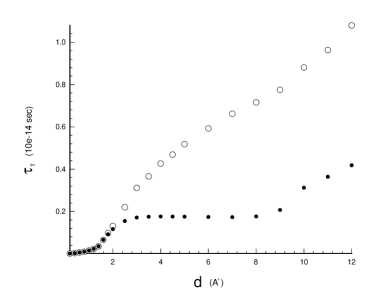
(c)

FIG. 2.: Diagrams (a), (b) and (c) show the dependence of the transmission time $\tau_{{}_{T}}$ in terms of the width of a square barrier with the height $V_{o}=10eV$ and the incident energy $E_{o}=\frac{\hbar^{2}k_{o}^{2}}{2m}=5eV$. These diagrams represent, respectively, Gaussian wave packets having the width $\sigma=6A^{o},\sigma=12A^{o}$ and $\sigma=18A^{o}$. We have shown the Bohmian results by hollow spheres and those of the standard interpretation by solid circles.

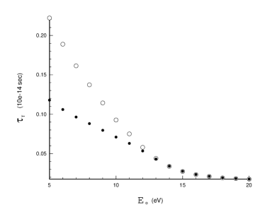
FIG. 3.: This diagram shows the transit time for a square barrier of width $b-a=3A^{o}$ and of height $V_{o}=10eV$, for Gaussian wave packets having $\sigma=12A^{o}$ and differents energies. We have shown Bohmian results by hollow spheres and those of the standard interpretation by solid circles.

IV Experimental test

It is generally believed that the standard quantum mechanics and Bohmian mechanics have identical predictions for physical observables. On the other hand, there is no Hermitian operator associated with time. Is it possible to consider a phenomenon involving time, e.g. tunneling, to differentiate between these two theories? By considering a thought experiment, Cushing gave a positive response to this question. His argument was the following [1, 2]:
(1) There is presently no satisfactory account of a quantum tunneling time (QTT) in the standard quantum mechanics.
(2) There is a well defined account of QTT in Bohmian interpretation. If it can be measured, then such a measurement would constitute a test of the interpretation .
(3) It might be possible to measure the Bohmian QTT with an experiment of a certain type.
(4) Therefore, from (2) and (3), if an experiment of that type is possible, such an experiment could serve as a test of Bohm’s interpretation.
(5) Because of (1), the outcome of an experiment of that type would not support or refute the copenhagen interpretation.
In a recent article, K. Bedard[2], by refering to (1), (2) and (5) questioned Cushing’s conclusion. Her argument was based on the fact that the two theories have different microontologies. Therefore, the QTT obtainable from Bohmian mechanics has no counterpart in the standard quantum mechanics. Thus, the measurement of such a time cannot be considered a test between the two theories. Here, we shall question (3), i.e. the claim that Cushing’s thought experiment can be used to measure Bohmian times.

Cushing’s experiment consists of a potential barrier between $x_{1}$ and $x_{2}$ with width $d$ ($d=b-a$). A detector $D_{T}$ is located at $x_{2}$ on the right of barrier and a detector $D_{R}$ is located at $x_{1}$ on the left of the barrier ($x_{1}<a<b<x_{2}$). Electrons are incident from the left. $D_{T}$ records the arrival times of the transmitted electrons at $x_{2}$ and $D_{R}$ records the times of the reflected electron at $x_{1}$. The distance from $x_{1}$ to the left side of the barrier ($a$) is a much more than width of wave packet. The same holds for $x_{2}$. The recording of the arrival time of the incident electron at $x_{1}$ will collapse the wave function. In that case, any subsequent tunneling time prediction on the basic of the known incident wave packet would be quite useless. To resolve this problem, Cushing considers the preparation of the state of the incident particle at $x_{1}$, rather than its detection. Thus, the time recorded at $x_{1}$ is the preparation time for the transit of the particle, if $D_{T}$ would detect it, and the preparation time for the reflected paticle, if $D_{R}$ would detect it. To provide this condition, we prepare a source of electrons in front of which there is a shutter. The shutter starts to open little before $t_{o}=0$ and closes little after $t_{o}$. Thus $t_{o}$ is the most probable time for the passage of the electron from $x_{1}$. In other words, $t_{o}$ is the time when the peak of the wave packet passes $x_{1}$. By choosing a weak source, we can be sure to have at most one electron emerging from shutter’s opening. The time of passage for the particle through $x_{1}$ is $t_{1}=t_{o}\pm\frac{\Delta x}{v_{o}}$, where $\Delta x$ is the widths of the packet and $v_{o}$ is the speed of the particle. Cushing claims that ” in principle, this error could be made as small as we like (for large enough $v_{o}$)”[1]. In our opinion, the error must be campared with $\tau_{{}_{T}}$ not with $t_{1}$. In fact, we want to obtain $\tau_{{}_{T}}$ which is the difference of the two time ($t_{2}-t_{1}$), where $t_{2}$ is the time that electron is detected at $x_{2}$ by $D_{T}$). The error could be small if we compare it with $t_{1}$ and $t_{2}$ but not if we compare it with their difference. Thus, we must have:

$$\frac{\Delta x}{v_{o}}\ll\tau_{{}_{T}}$$ (40)

By refering to the Fig.(3), one can see that $\tau_{{}_{T}}$ decreases quicker than $\frac{1}{v_{o}}$. Thus, the increase in $v_{o}$ decreases the right hand side of (23) more than its left hand side and we are not able to decrease relative error in this way. One may hope obtaining condition (23) by decreasing $\Delta x$. But decreasing $\Delta x$ is not useful. Because, by refering to Fig.(2) (a, b, c) one can see that $\tau_{{}_{T}}$ decreases almost linearly with $\Delta x$.

Experimental limitations dictate that the arrival time of particles to the barrier be measured independent of whether they shall be reflected or transmitted (i.e. state preparation time). Thus, although Bohm’s theory considers $\tau_{{}_{in}}^{{}^{T}}$ and $\tau_{{}_{in}}^{{}^{R}}$, it must pay attention only to the measurements of $\tau_{{}_{in}}=|T|^{2}\tau_{{}_{in}}^{{}^{T}}+|R|^{2}\tau_{{}_{in}}^{{}^{R}}$, to avoid experimental limitations. In this way, the precise time that it attributes to particle’s transmission through the barrier or reflection is $\tau_{{}_{T}}^{{}^{OR}}$ and $\tau_{{}_{R}}^{{}^{OR}}$ respectively. Thus, at the experimental level, even in the case of tunneling times we have the same predictions in the two theories. In fact, here, we encounter a problem like the case of the celebrated two-slit experiment. In the framework of Bohmian mechanics, all particles observed on the lower (upper) half of the screen must come from the lower (upper) slit. But, any effort to know which particle came from which slit destroys the interference pattern. Thus, in the two-slit experiment, the two theory come to the same result due to experimental limitations. It appears that, from various definitions given for QTT in the framework of the standard quantum mechanics, our choice of OR’s is the best. Because, in our opinion it is the best time that can be related to the tunneling phenomena in the framework of the standard interpretation of quantum mechanics. We can justify our claim in the follow way:
(1) There is a unique and well defined account of QTT in Bohm’s interpretation.
(2) There are several accounts of QTT in standard interpretation.
(3) These two theories have the same prediction for observables.
(4) Bohmian prediction for QTT coincides with one of Copenhagen QTT (OR’s).

In fact, OR’s is the only definition that gives the same result, at the experimental level, as Bohmian mechanics, although it does not associate an operator with $\tau_{{}_{T}}$ (at least up to now). In this way, we have used a theory with additional microontology (Bohmian mechanics) to give the best definition for a quantity in a theory with less microontology. Bohm’s theory may also shed light on other definitions of QTT in the standard quantum mechanics.

Conclusion

Considering the fact that the microontology of Copenhagen theory includes wave function (probability amplitude), and not point-like particles, the best time one could attribute to the passage of a particle from a point of space is the average time of the passage of probability flux (eq.(3)). Generalization of this time to QTT, leads one to OR’s times. On other hand, the microontology of Bohmian mechanics includes point-like particles in addition to wave function, and it leads uniquely to Bohmian QTT (eq.(18)). We have compared them for different width and energy of wave packet in Fig.(2) and Fig.(3) by use of numerical calculation.

Now, Bohmian QTT could not be measured due to experimental limitations. The best times that could be obtained in Bohmian mechanics are the same as OR’s. The agreement of one of the several available definitions of QTT in Copenhagen quantum mechanics with the unique definition of Bohmian mechanics, separates it from others. Because, it is reasonable to expect same prediction for the two theories even in the case of QTT.

Acknowledgments

The authors would like to thank Dr. C. R. Leavens drawing our attention to prior work of Olkhovsky and Recami.

REFERENCES

- [1] Cushing, J. T., Found. Phys. 25, 1995, 269.
- [2] Bedard, K., Found. Phys. Lett. 10, 1997, 183.
- [3] Ranfagni, A., Mugnai, P., Fabeni, P. and Pazzi, G. P., Appl. Phys. Lett. 58, 1990, 774.
- [4] Capasso, F. and Mohammed, K., Cho, A.Y., IEEEJ. Quantum Electron. QE22, 1986, 1853.
- [5] Baz, A.L., Sov. J. Nucl. Phys. 4, 1967, 182.
- [6] Rybachenko, V.F., Sov. J. Nucl. Phys. 5, 1967, 635.
- [7] Büttiker, M., Phys. Rev. B27, 1983, 6178.
- [8] Falck, J.P. and Hauge, E.H., Phys. Rev. B38, 1988, 3287.
- [9] Sokolorski, D. and Baskin, L.M., Phys. Rev. A36, 1987, 4604.
- [10] Hauge, E. H., Falck, J.P., and Fjeldly, T.A., Phys. Rev B36, 1987, 4203.
- [11] Jaworski, W. and Wardlaw, D.M., Phys. Rev. A37, 1988, 2843.
- [12] Ming-Quey Chen and Wang, M.S., Phys. Lett. B149, 1990, 441.
- [13] Yücel, S. and Andrei, Eva Y., Phys. Rev. B46, 1992, 2448.
- [14] Fertig, H.A., Phys. Rev. Lett. 65, 1990, 234.
- [15] Hagmann, M.J., Solid State Commun. 82, 1992, 867.
- [16] Delgado, V. and Muga, J.G., Phys. Rev. A56, 1997, 3425.
- [17] Landauer, R. and Martin, Th., Rev. Mod. Phys. 66, 1994, 217.
- [18] Hauge, E. H. and Stovneng, J.A., Rev. Mod. Phys. 61, 1989, 917.
- [19] Bohm, D., Phys. Rev. 85, 1952, 166-193.
- [20] Leavens, C.R., Solid State Commun. 74, 1990, 923 and 76, 1990, 253.
- [21] Leavens, C.R., Found. Phys. 25, 1995, 229.
- [22] Dumont, R.S. and Marchioro, T.L., Phys. Rev. A47, 1993, 85.
- [23] Leavens, C.R., Phys. Lett. A178, 1993, 27.
- [24] Olkhovsky, V.S. and Recami, E., Phys. Rep. 214, 1992, 339.
- [25] Olkhovsky, V.S., Recami, E. and Zaichenko, A.K., Solid State Commun. 89, 1994, 31.
- [26] Leavens, C.R., Solid State Commun. 85, 1993, 115.
- [27] Delgado, V., Brouard, S. and Muga, J.G.,, Solid State Commun. 94, 1995, 979.
- [28] De Readt, H., Computer Physics Reports. 7, 1987, 1.
- [29] Brouard, S., Sala, R. and Muga, J.G.,, Phys. Rev. A 49 , 1994, 4312.