Stochastic wave function method for non-Markovian quantum master equations

Abstract

A generalization of the stochastic wave function method to quantum master equations which are not in Lindblad form is developed. The proposed stochastic unravelling is based on a description of the reduced system in a doubled Hilbert space and it is shown, that this method is capable of simulating quantum master equations with negative transition rates. Non-Markovian effects in the reduced systems dynamics can be treated within this approach by employing the time-convolutionless projection operator technique. This ansatz yields a systematic perturbative expansion of the reduced systems dynamics in the coupling strength. Several examples such as the damped Jaynes Cummings model and the spontaneous decay of a two-level system into a photonic band gap are discussed. The power as well as the limitations of the method are demonstrated.

I Introduction

The theory of open quantum systems is a fundamental approach to the understanding of dissipation on a microscopic and macroscopic level in many fields of physics, such as quantum optics, and solid state physics. Besides the conventional density matrix formalism, there has been an increasing interest over the last years in the stochastic wave function method [1, 2, 3, 4, 5, 6], where the state of the open system is described by an ensemble of pure states instead of a reduced density matrix. This method permits a description of the dynamics of an individual quantum system subject to a continuous measurement [7, 8] and hence provides additional information about the state of the system compared to the description by a reduced density matrix. Moreover, the stochastic wave functions method has been shown to be an effective numerical tool for the solution of density matrix equations with many degrees of freedom since a reduced density matrix has $N^{2}$ degrees of freedom, whereas a stochastic wave vector only has $N$ components [9, 10].

Since the stochastic wave function method originated in the context of quantum optics most publications on this subject consider the weak coupling regime and the Born-Markov approximation seems to be inevitably connected with this approach. On the other hand, the stochastic wave functions method could also provide a useful numerical tool in other fields of physics, where the Born-Markov approximation is not justified. This has been shown for example by Imamoglu [11], who extended the stochastic wave function method to the strong coupling regime by considering an enlarged system which contains a few ficticious bath-modes, that are weakly coupled to a Markovian environment. Although this concept is quite general, the drawback of this method is obvious: even if the state space of the system is small, the numerical treatment of the enlarged system can become very expensive if more than a few ficticious modes are needed to approximate the reduced systems dynamics. Another approach to a non–Markovian stochastic wave function method developed by Jack, Collett and Walls [12] is based on a continuous measurement interpretation of the stochastic unraveling. In this approach the stochastic equation of motion for the reduced state vector involves a multiple time integration over the system’s history conditioned on the measurement record over a finite time interval. Furthermore, it has been claimed recently by Diósi et al. [13, 14] that it is in principle possible to construct an exact stochastic Schrödinger equation which describes the non-Markovian time evolution of an open quantum system.

In this article we present an extension of the stochastic wave function method beyond the Born-Markov approximation which is based on the time-convolutionless projection operator technique [15, 16]. This ansatz yields a systematic perturbative expansion scheme for the stochastic dynamics of the reduced system which is valid in an intermediate coupling regime where non-Markovian effects are important, but a perturbative expansion is still justified. The major advantage of our method is that it does not rely on an enlarged phase space and that it uses a stochastic evolution equation which is local in time.

The paper is organized as follows. In Sec. II we briefly review three different approaches to equations of motion for the reduced density matrix: the derivation of the Markovian quantum master equation (Sec. II A), the Nakajima-Zwanzig projection operator technique (Sec. II B), which yields a generalized master equation, and the time-convolutionless projection operator technique (Sec. II C), leading to a quantum master equation which is local in time. Sec. III deals with the stochastic unravelling of quantum master equations: in Sec. III A we review the stochastic unravelling of quantum master equations which are in Lindblad form, such as the Markovian quantum master equation, whereas in Sec. III B we present an unravelling of arbitrary linear density matrix equations which are local in time, such as the time-convolutionless quantum master equation. These algorithms are then applied to the damped Jaynes-Cummings model and the spontaneous decay of a two-level system into a photonic band gap in Sec. IV. Sec. V contains our summary.

II Derivations of quantum master equations

We shall begin with a description of the models we want to examine and state the basic assumptions underlying the following sections. Throughout this article, we consider a quantum mechanical system S which is coupled to a reservoir R. The combined system is supposed to be closed and its Hamiltonian is of the form

$$H=H_{0}+\alpha H_{\rm I},$$ (1)

where $H_{0}$ is the Hamiltonian of the system and the reservoir and $H_{\rm I}$ the interaction Hamiltonian. The time evolution of the combined system’s density matrix in the interaction picture $W(t)$ is determined by the Liouville-von Neumann equation

$$\frac{\partial}{\partial t}W(t)=-i\alpha[H_{\rm I}(t),W(t)]\equiv\alpha L(t)W(t),$$ (2)

where the interaction Hamiltonian in the interaction picture is defined as $H_{\rm I}(t)=\exp(iH_{0}t)H_{\rm I}\exp(-iH_{0}t)$. The initial state of the combined system is supposed to factorize,

$$W(0)=\rho(0)\otimes\rho_{\rm R},$$ (3)

where $\rho_{\rm R}$ is some stationary state of the reservoir, i. e., the system and the reservoir are initially uncorrelated. For technical simplicity, we further assume that odd moments of $H_{\rm I}(t)$ with respect to $\rho_{\rm R}$ vanish, i. e.,

$$\mbox{Tr}_{\rm R}\left\{\rho_{\rm R}H_{\rm I}(t_{1})\cdots H_{\rm I}(t_{2k+1})\right\}=0,$$ (4)

although this assumption is not essential for the methods we want to use in this article (see Ref. [15]).

Since Eq. (2) is in general a system of (infinitely) many differential equations, exact solutions are only known in rare cases. Moreover, even if an exact solution can be found, one is usually not interested in the dynamics of the environment but wants to calculate the time evolution of system observables. Therefore, we seek an approximate equation of motion for the reduced density matrix $\rho(t)=\mbox{Tr}_{\rm R}\{W(t)\}$ of the open system. In this section we will describe three different approaches to that goal: the Born-Markov approximation, the Nakajima-Zwanzig projection operator technique and the time-convolutionless projection operator technique.

A The Markovian quantum master equation

In this section we sketch an intuitive derivation of the Markovian quantum master equation based on the Born-Markov approximation (see, e. g., [17, 18]). The starting point is an exact equation of motion for the reduced density matrix which can be obtained by integrating the Liouville-von Neumann equation (2) twice, differentiating with respect to $t$ and taking the trace over the reservoir. This yields the exact equation of motion

$$\dot{\rho}(t)=-\alpha^{2}\int_{0}^{t}ds\,\mbox{Tr}_{\rm R}\left\{\left[H_{\rm I}(t),\left[H_{\rm I}(s),W(s)\right]\right]\right\},$$ (5)

which still contains the density matrix $W(t)$ of the composed system.

The first approximation we make is the Born approximation which consists in approximating the density matrix of the composed system by a product of the form

$$W(t)\approx\rho(t)\otimes\rho_{\rm R},$$ (6)

where $\rho(t)$ refers to the variables of the reduced system and $\rho_{\rm R}$ denotes a stationary state of the environment. Such an approximation is justified if the coupling between the system and the environment is weak. Inserting Eq. (6) into Eq. (5) we obtain the closed integro-differential equation for the reduced density matrix

$$\dot{\rho}(t)=-\alpha^{2}\int_{0}^{t}ds\,\mbox{Tr}_{\rm R}\left\{\left[H_{\rm I}(t),\left[H_{\rm I}(s),\rho(s)\otimes\rho_{\rm R}\right]\right]\right\}.$$ (7)

This equation is further simplified by making the Markov approximation: replacing $\rho(s)$ by $\rho(t)$ yields a closed differential equation of motion for the reduced density matrix which contains only $\rho(t)$, namely

$$\dot{\rho}(t)=-\alpha^{2}\int_{0}^{t}ds\,\mbox{Tr}_{\rm R}\left\{\left[H_{\rm I}(t),\left[H_{\rm I}(s),\rho(t)\otimes\rho_{\rm R}\right]\right]\right\}.$$ (8)

The Markov approximation is based on the assumption that the correlation time of the reservoir $\tau_{\rm R}$ is small compared to the time scale $\tau_{\rm S}$ on which $\rho(t)$ changes. The final form of the quantum master equation is obtained by extending the upper limit of the integral to infinity, which is valid for times $t\gg\tau_{\rm R}$ since the integrand is negligible for $s\gg\tau_{\rm R}$.

Within this derivation of the quantum master equation, the Markov approximation appears as an additional approximation besides the Born approximation, and one is tempted to believe, that the generalized master equation (7) is more accurate than the master equation (8). However, as we will see in Secs. II B and II C, both approximations are only valid to second order in the coupling strength $\alpha$ and are hence equally accurate (see also [19, 20]). We will also demonstrate this by means of a specific example in Sec. IV B.

B Nakajima-Zwanzig projection operator technique

The Nakajima-Zwanzig projection operator technique [21, 22, 23] is based on a partition of the state of a system into a relevant and an irrelevant part by defining an adequate projection operator ${\cal P}$ which projects the state on the relevant part and a projector ${\cal Q}=1-{\cal P}$ which projects on the irrelevant part. For our system reservoir model we define the projector ${\cal P}$ in the usual way as

$${\cal P}W(t)=\mbox{Tr}_{\rm R}\left\{W(t)\right\}\otimes\rho_{\rm R}\equiv\rho(t)\otimes\rho_{\rm R},$$ (9)

where $\rho_{\rm R}$ is a stationary state of the reservoir. The equation of motion for the two components ${\cal P}W(t)$ and ${\cal Q}W(t)$ can be obtained directly form the Liouville-von Neumann equation (2):

$$\frac{\partial}{\partial t}{\cal P}W(t) = \alpha{\cal P}L(t){\cal P}W(t)+\alpha{\cal P}L(t){\cal Q}W(t)$$ (10)

$$\frac{\partial}{\partial t}{\cal Q}W(t) = \alpha{\cal Q}L(t){\cal P}W(t)+\alpha{\cal Q}L(t){\cal Q}W(t).$$ (11)

Taking into account the initial condition Eq. (3) the formal solution of Eq. (11) reads

$${\cal Q}W(t)=\alpha\int_{0}^{t}ds\,{\cal G}(t,s){\cal Q}L(s){\cal P}W(s)$$ (12)

where ${\cal G}(t,s)$ is defined as

$${\cal G}(t,s)=T_{\leftarrow}\exp\left(\alpha\int_{s}^{t}ds^{\prime}\,{\cal Q}L(s^{\prime})\right).$$ (13)

The symbol $T_{\leftarrow}$ indicates the chronological time ordering. Substituting the expression for ${\cal Q}W(t)$ into the equation of motion of the relevant part of the state (10) we obtain the generalized master equation for ${\cal P}W(t)$

$$\frac{\partial}{\partial t}{\cal P}W(t)=\alpha{\cal P}L(t){\cal P}W(t)+\int_{0}^{t}ds\,\widetilde{K}(t,s){\cal P}W(s),$$ (14)

with the memory kernel

$$\widetilde{K}(t,s)=\alpha^{2}{\cal P}L(t){\cal G}(t,s){\cal Q}L(s).$$ (15)

It is important to note, that the generalized master equation (14) is exact and that, hence, the explicit computation of the memory kernel $\widetilde{K}(t,s)$ is, in general, as complicated as the explicit solution of the Liouville-von Neumann equation (2). However, Eq. (14) serves as a starting point for systematic approximations. For example, a perturbative expansion of the memory kernel $\widetilde{K}(t,s)$ to second order in the coupling strength $\alpha$ leads to the generalized quantum master equation in the Born approximation (7). On the other hand, although the computation of the memory kernel is essentially facilitated by using a perturbative expansion, the final form of the equation of motion is still an integro-differential equation, the integration of which can be rather difficult. We can overcome this by using the time-convolutionless projection operator technique, which will be described in the following Section.

C Time-convolutionless projection operator technique

The basic idea of the time-convolutionless projection operator technique [15, 16] is to replace $W(s)$ in the formal solution of the irrelevant part (12) by

$$W(s)=G(t,s)({\cal P}+{\cal Q})W(t),$$ (16)

where the backward propagator $G(t,s)$ of the composite system is defined as

$$G(t,s)=T_{\rightarrow}\exp\left(-\alpha\int_{s}^{t}ds^{\prime}\,L(s^{\prime})\right),$$ (17)

and $T_{\rightarrow}$ indicates the anti-chronological time ordering. Solving Eq. (16) for ${\cal Q}W(t)$, we find

$${\cal Q}W(t)=\left[1-\Sigma(t)\right]^{-1}\Sigma(t){\cal P}W(t),$$ (18)

with

$$\Sigma(t)=\alpha\int_{0}^{t}ds{\cal G}(t,s){\cal Q}L(s){\cal P}G(t,s),$$ (19)

which can be substituted in Eq. (10) to obtain the exact, time-convolutionless equation of motion for the relevant part of the system

$$\frac{\partial}{\partial t}{\cal P}W(t) = K(t){\cal P}W(t)$$ (20)

$$\equiv \alpha{\cal P}L(t)\left[1-\Sigma(t)\right]^{-1}{\cal P}W(t).$$ (21)

The crucial point of this construction is the existence of the generator $K(t)$ which relies on the existence of the operator $\left[1-\Sigma(t)\right]^{-1}$. Since $\Sigma(0)=0$ and $\Sigma(t)$ is continuous, this operator exists for all $t$ if and only if it can be expanded in a geometric series

$$\left[1-\Sigma(t)\right]^{-1}=\sum_{n=0}^{\infty}\Sigma(t)^{n}.$$ (22)

This condition is always satisfied for short times or in the weak coupling regime, but can be violated in the strong coupling regime, as will be demonstrated explicitly in Sec. IV B. Therefore, we define the intermediate coupling regime as the range of coupling parameters $\alpha$, where non-Markovian effects are significant, but the generator $K(t)$ exists for all $t$.

Using Eq. (22) we can also write the generator of the time-convolutionless master equation as

$$K(t)=\sum_{n=0}^{\infty}\alpha{\cal P}L(t)\Sigma(t)^{n}.$$ (23)

This form is the starting point for a perturbative expansion of $K(t)$ in powers of the coupling strength $\alpha$. To fourth order one obtains, for example,

$$K(t)=\alpha^{2}K_{2}(t)+\alpha^{4}K_{4}(t)+{\cal O}(\alpha^{6})$$ (24)

where

$$K_{2}(t)=\int_{0}^{t}dt_{1}{\cal P}L(t)L(t_{1}){\cal P},$$ (25)

and

$$K_{4}(t)=\int_{0}^{t}dt_{1}\int_{0}^{t_{1}}dt_{2}\int_{0}^{t_{2}}dt_{3}$$ (28)

$$\times\Big{[}{\cal P}L(t)L(t_{1})L(t_{2})L(t_{3}){\cal P}-{\cal P}L(t)L(t_{1}){\cal P}L(t_{2})L(t_{3}){\cal P}$$

$$-{\cal P}L(t)L(t_{2}){\cal P}L(t_{1})L(t_{3}){\cal P}-{\cal P}L(t)L(t_{3}){\cal P}L(t_{1})L(t_{2}){\cal P}\Big{]}.$$

The higher–order terms can be obtained in a way similar to van Kampen’s cumulant expansion [19, 24]. All terms containing odd orders of the coupling strength vanish in this expansion, since by definition of ${\cal P}$ and $L(t)$ we have ${\cal P}L(t_{1})\cdots L(t_{2k+1}){\cal P}=0$ (see Eq. (4)). It is important to note that the general structure of the time-convolutionless equation of motion (20) of the reduced density matrix is not changed by the perturbative expansion, i. e., the approximative equation of motion is also linear in $\rho(t)$ and local in time, unlike the perturbative expansion of the generalized master equation (14).

1 The equation of motion to second order

When we substitute the expressions for the generator $L(t)$ and the projection operator ${\cal P}$, Eqs. (2) and (9), respectively, into the second order contribution to $K(t)$ we immediately obtain the time-dependent quantum master equation (8) within the Born-Markov approximation (without extending the upper limit of the time integration to infinity). Thus, Eq. (7) as well as Eq. (8) are correct to the same order in the coupling and the major approximation in the heuristic derivation of the quantum master equation in Sec. II A is not the Markov, but the Born approximation. This seems to be somewhat counterintuitive, since after making the Born approximation the equation of motion of the reduced density matrix is still a complicated integro-differential equation, whereas the Markov approximation considerably simplifies the calculations. Nevertheless, it does in general not improve the accuracy of a calculation to make only the Born-approximation and to omit the Markov-approximation.

2 The equation of motion to fourth order

We now compute the explicit expression $K_{4}(t)$ for the fourth order contribution to the time-convolutionless equation of motion. To this end, we decompose the interaction Hamiltonian into a sum of products in the form

$$H_{\rm I}=\sum_{k}F_{k}\otimes Q_{k}.$$ (29)

We further assume, that the state $\rho_{\rm R}$ is not only stationary, but also Gaussian, i. e.,

$$\mbox{Tr}_{\rm R}\left\{\rho_{\rm R}Q_{i_{0}}(t)Q_{i_{1}}(t_{1})Q_{i_{2}}(t_{2})Q_{i_{3}}(t_{3})\right\}=$$ (31)

$$\mbox{Tr}_{\rm R}\left\{\rho_{\rm R}Q_{i_{0}}(t)Q_{i_{1}}(t_{1})\right\}\mbox{Tr}_{\rm R}\left\{\rho_{\rm R}Q_{i_{2}}(t_{2})Q_{i_{3}}(t_{3})\right\}$$

$$+ \mbox{Tr}_{\rm R}\left\{\rho_{\rm R}Q_{i_{0}}(t)Q_{i_{2}}(t_{2})\right\}\mbox{Tr}_{\rm R}\left\{\rho_{\rm R}Q_{i_{1}}(t_{1})Q_{i_{3}}(t_{3})\right\}$$ (32)

$$+ \mbox{Tr}_{\rm R}\left\{\rho_{\rm R}Q_{i_{0}}(t)Q_{i_{3}}(t_{3})\right\}\mbox{Tr}_{\rm R}\left\{\rho_{\rm R}Q_{i_{1}}(t_{1})Q_{i_{2}}(t_{2})\right\},$$ (33)

and we introduce the short-hand notation

$$\hat{0},\hat{1},\cdots \qquad\mbox{ denotes }F_{i_{0}}(t),F_{i_{1}}(t_{1}),\cdots$$

$$\langle 12\rangle,\cdots \qquad\mbox{ denotes }\mbox{Tr}_{\rm R}\left\{\rho_{\rm R}Q_{i_{1}}(t_{1})Q_{i_{2}}(t_{2})\right\},\cdots$$

and sum over repeated indices $i_{k}$. In this notation we find for example

$${\cal P}L(t)\cdots L(t_{3}){\cal P}W(t)$$ (34)

$$= \left[\hat{0},\left[\cdots,\left[\hat{3},\rho\right]\cdots\right]\right]\langle 0\cdots 3\rangle$$ (35)

$$= \sum_{i_{0}\cdots i_{3}}\left[F_{i_{0}}(t),\left[\cdots,\left[F_{i_{3}}(t_{3}),\rho(t)\right]\cdots\right]\right]$$ (37)

$$\times\mbox{Tr}_{\rm R}\left\{\rho_{\rm R}Q_{i_{0}}(t)\cdots Q_{i_{3}}(t_{3})\right\},$$

and inserting the expression (29) into Eq. (28), we obtain

$$K_{4}(t){\cal P}W(t)=\int_{0}^{t}dt_{1}\int_{0}^{t_{1}}dt_{2}\int_{0}^{t_{2}}dt_{3}$$ (43)

$$\times\big{\{}\langle 02\rangle\langle 13\rangle\left[\hat{0},\left[\hat{1},\hat{2}\right]\hat{3}\rho\right]-\langle 02\rangle\langle 31\rangle\left[\hat{0},\left[\hat{1},\hat{2}\right]\rho\hat{3}\right]$$

$$-\langle 20\rangle\langle 13\rangle\left[\hat{0},\hat{3}\rho\left[\hat{1},\hat{2}\right]\right]+\langle 20\rangle\langle 31\rangle\left[\hat{0},\rho\hat{3}\left[\hat{1},\hat{2}\right]\right]$$

$$+\langle 03\rangle\langle 12\rangle\left(\left[\hat{0},\left[\hat{3},\hat{2}\right]\rho\hat{1}\right]+\left[\hat{0},\left[\hat{1}\hat{2},\hat{3}\right]\rho\right]\right)$$

$$+\langle 30\rangle\langle 21\rangle\left(\left[\hat{0},\hat{1}\rho\left[\hat{3},\hat{2}\right]\right]+\left[\hat{0},\rho\left[\hat{2}\hat{1},\hat{3}\right]\right]\right)$$

$$-\langle 03\rangle\langle 21\rangle\left[\hat{0},\left[\hat{1},\hat{3}\right]\rho\hat{2}\right]-\langle 30\rangle\langle 12\rangle\left[\hat{0},\hat{2}\rho\left[\hat{1},\hat{3}\right]\right]\big{\}}.$$

Note that this expression contains commutators between various system operators, which can immensely simplify the explicit evaluation of $K_{4}(t)$, if certain commutation relations are specified, such as bosonic commutation relations for a harmonic oscillator, or the commutation relations for the pseudospin operators (see Sec. IV A).

III Stochastic unravelling of quantum master equations

A Quantum master equations in Lindblad form

In Ref. [25] Lindblad has shown that the equation of motion of a reduced density matrix has to be of the form

$$\frac{\partial}{\partial t}\rho(t)=-i\left[H_{\rm S}+\frac{1}{2}\sum_{i}S_{i}(t)L_{i}^{\dagger}L_{i},\rho(t)\right]$$ (44)

$$+ \sum_{i}\gamma_{i}(t)\left\{-\frac{1}{2}L_{i}^{\dagger}L_{i}\rho(t)-\frac{1}{2}\rho(t)L_{i}^{\dagger}L_{i}+L_{i}\rho(t)L_{i}^{\dagger}\right\},$$ (45)

if the dynamics of the reduced system is assumed to conserve positivity and to represent a quantum dynamical semi-group. Here, $H_{\rm S}$ is the Hamiltonian of the system, the time-dependent coefficients $S_{i}(t)$ describe an energy shift induced by the coupling to the environment, namely the Lamb and Stark shifts, and the positive rates $\gamma_{i}(t)$ model the dissipative coupling to the $i-$th decay channel.

In this case, the state of the open system can alternatively be described by a stochastic wave function $\psi(t)$ [1, 2, 3, 4, 5, 6], the covariance matrix of which equals the reduced density matrix, i. e.,

$$\rho(t)=\int D\psi D\psi^{*}\,|\psi\rangle\langle\psi|P[\psi,t],$$ (46)

where $P[\psi,t]$ is the probability density functional of finding the state of the open system in the Hilbert space volume element $D\psi D\psi^{*}$ at the time $t$ [26, 27].

The time evolution of the stochastic wave function is governed by a stochastic differential equation, which might either be diffusive [5, 6] or of the piecewise deterministic jump type [1, 2, 3, 4]. The latter takes the form [7]

$$d\psi(t)=-iG(\psi,t)dt+\sum_{i}\left(\frac{L_{i}\psi(t)}{\|L_{i}\psi(t)\|}-\psi(t)\right)dN_{i}(t),$$ (47)

where the $dN_{i}(t)$ are the differentials of independent Poisson process $N_{i}(t)$ with mean $\langle dN_{i}(t)\rangle=\gamma_{i}(t)\|L_{i}\psi(t)\|^{2}dt$. The drift generator takes the form

$$G(\psi,t) = H(t)\psi+\frac{1}{2}\sum_{i}S_{i}(t)L_{i}^{\dagger}L_{i}\psi$$ (49)

$$-\frac{i}{2}\sum_{i}\gamma_{i}(t)\left(L_{i}^{\dagger}L_{i}-\|L_{i}\psi\|^{2}\right)\psi.$$

For the differential of the Poisson process $dN_{i}(t)$ the Ito rule $dN_{i}(t)dN_{j}(t)=\delta_{ij}dN_{i}(t)$ holds, that is, $dN_{i}(t)$ can either be $0$ or $1$. If $dN_{i}(t)=0$, then the system evolves continuously according to the nonlinear Schrödinger-type equation

$$i\frac{\partial}{\partial t}\psi(t)=G(\psi,t),$$ (50)

whereas, if $dN_{i}(t)=1$ for some $i$, then the system undergoes an instantaneous, discontinuous transition of the form

$$\psi(t)\longrightarrow\frac{L_{i}\psi(t)}{\|L_{i}\psi(t)\|}.$$ (51)

Note that the generator $G(\psi,t)$ of the continuous time evolution is non-Hermitian and hence the propagator of $\psi(t)$ is non-unitary. However, due to the nonlinearity of the generator, the norm of $\psi(t)$ is preserved in time.

Using the Ito calculus for the differentials $dN_{i}(t)$ it is easy to check that the equation of motion of the covariance matrix of $\psi(t)$ equals the usual Markovian quantum master equation (44) in Lindblad form. Thus, expectation values of system observables can either be calculated by means of the reduced density matrix or as averages over different realizations of the stochastic process $\psi(t)$ and both descriptions yield the same results.

B General quantum master equations

The most general type of a quantum master equation which results from the time-convolutionless projection operator technique – or from a perturbative approximation – is linear in $\rho(t)$ and local in time (see Sec. II C) but needs not to be in the Lindblad form, as we will show in an example below (see Sec. IV C). However, these equations can always be written in the form

$$\frac{\partial}{\partial t}\rho(t)=A(t)\rho(t)+\rho(t)B^{\dagger}(t)+\sum_{i}C_{i}(t)\rho(t)D_{i}^{\dagger}(t),$$ (52)

with some time-dependent linear operators $A(t)$, $B(t)$, $C_{i}(t)$, and $D_{i}(t)$. In order to find an unraveling of this equation of motion we follow a strategy, which has already been successfully applied to the calculation of multitime correlation functions [28, 29]. We describe the state of the open system by a pair of stochastic wave functions

$$\theta(t)=\left(\begin{array}[]{c}\phi(t)\\ \psi(t)\end{array}\right).$$ (53)

Formally, $\theta(t)$ can be regarded as an element of the doubled Hilbert space $\widetilde{\cal H}={\cal H}\oplus{\cal H}$. If $\widetilde{P}[\theta,t]$ denotes the probability density functional of the process in the doubled Hilbert space $\widetilde{\cal H}$, we may define the reduced density matrix as

$$\rho(t)=\int D\theta D\theta^{*}|\phi\rangle\langle\psi|\widetilde{P}[\theta,t].$$ (54)

The time evolution of the state vector $\theta(t)$ is then governed by the stochastic differential equation

$$d\theta(t) = -iG(\theta,t)dt$$ (56)

$$+\sum_{i}\left(\frac{\|\theta(t)\|}{\left\|J_{i}(t)\theta(t)\right\|}J_{i}(t)\theta(t)-\theta(t)\right)dN_{i}(t),$$

where $dN_{i}(t)$ is the differential of a Poisson process with mean

$$\langle dN_{i}(t)\rangle=\frac{\left\|J_{i}(t)\theta(t)\right\|^{2}}{\|\theta(t)\|^{2}}dt,$$ (57)

and the functional $G(\theta,t)$ is defined as

$$G(\theta,t)=i\left(F(t)+\frac{1}{2}\sum_{i}\frac{\left\|J_{i}(t)\theta(t)\right\|^{2}}{\|\theta(t)\|^{2}}\right)\theta(t),$$ (58)

with the time-dependent operators

$$F(t)=\left(\begin{array}[]{cc}A(t)&0\\ 0&B(t)\end{array}\right),\quad J_{i}(t)=\left(\begin{array}[]{cc}C_{i}(t)&0\\ 0&D_{i}(t)\end{array}\right).$$ (59)

Again, this type of stochastic evolution equation describes a piecewise deterministic jump process, where the deterministic pieces are solutions of the differential equation

$$i\frac{\partial}{\partial t}\theta(t)=G(\theta,t),$$ (60)

and the jumps induce transitions of the form

$$\theta(t)\longrightarrow\frac{\|\theta(t)\|}{\|J_{i}\theta(t)\|}J_{i}\theta(t)=\frac{\|\theta(t)\|}{\|J_{i}\theta(t)\|}\left(\begin{array}[]{c}C_{i}\phi\\ D_{i}\psi\end{array}\right).$$ (61)

Note, that the structure of the stochastic differential equation in the doubled Hilbert space (56) is very similar to the structure of the stochastic differential equation (47). In fact, the unraveling of general quantum master equations presented in this section contains as a special case the unraveling of Lindblad–type equations shown in Sec. III A: If we set

$$A(t)=B(t)=-iH_{\rm S}-\frac{1}{2}\sum_{k}\left[\gamma_{k}(t)+iS_{k}(t)\right]L_{k}^{\dagger}L_{k}$$ (62)

and

$$C_{i}(t)=D_{i}(t)=\sqrt{\gamma(t)}L_{i},$$ (63)

the equation of motion (52) reduces to the Lindblad equation (44) and both unravelings are identical.

IV Example: The spontaneous decay of a two-level system

In this section we consider as an example of the general theory the exactly solvable model of a two-level system spontaneously decaying into the vacuum within the rotating wave approximation. The Hamiltonian of the total system is given by

$$H_{\rm 0} = \omega_{\rm S}\sigma^{+}\sigma^{-}+\sum_{k}\omega_{k}b_{k}^{\dagger}b_{k},$$ (64)

$$H_{\rm I} = \sigma^{+}\otimes B+\sigma^{-}\otimes B^{\dagger}\mbox{ with }B=\sum_{k}g_{k}b_{k},$$ (65)

where $\omega_{\rm S}$ denotes the transition frequency of the two-level system, the index $k$ labels the different field modes with frequency $\omega_{k}$, annihilation operator $b_{k}$ and coupling constant $g_{k}$, and $\sigma^{\pm}$ denote the pseudospin operators.

A Exact and approximated equations of motions

The exact solution and equation of motion for this model can be obtained in the following way: Define the states [30]

$$\psi_{0} = |0\rangle_{\rm S}\otimes|0\rangle_{\rm R}$$ (66)

$$\psi_{1} = |1\rangle_{\rm S}\otimes|0\rangle_{\rm R}$$ (67)

$$\psi_{k} = |0\rangle_{\rm S}\otimes|k\rangle_{\rm R}$$ (68)

where $|0\rangle_{\rm S}$ and $|1\rangle_{\rm S}$ indicate the ground and excited state of the system, respectively, the state $|0\rangle_{\rm R}$ denotes the vacuum state of the reservoir, and $|k\rangle_{\rm R}=b_{k}^{\dagger}|0\rangle_{\rm R}$ denotes the state with one photon in mode $k$. Since the interaction Hamiltonian conserves the total number of particles, the flow of the Schrödinger equation generated by $H_{\rm I}$ is confined to the subspace spanned by these vectors. Hence, we may expand the state of the total system at any time as

$$\phi(t)=c_{0}\psi_{0}+c_{1}(t)\psi_{1}+\sum_{k}c_{k}(t)\psi_{k},$$ (69)

with some probability amplitudes $c_{0}$, $c_{1}(t)$, and $c_{k}(t)$. The time evolution of these probability amplitudes is determined by a complicated system of ordinary differential equations, which can be solved in some simple cases by introducing the so-called pseudomodes [30]. With these probability amplitudes, the reduced density matrix takes the form

$$\rho(t)=\left(\begin{array}[]{cc}|c_{1}(t)|^{2}&c_{1}(t)c_{0}^{*}\\ c_{1}^{*}(t)c_{0}&|c_{0}|^{2}+\sum_{k}|c_{k}(t)|^{2}\end{array}\right).$$ (70)

Differentiating this expression with respect to time we get the following exact equation of motion,

$$\frac{\partial}{\partial t}\rho(t)=-\frac{i}{2}S(t)[\sigma^{+}\sigma^{-},\rho(t)]$$ (72)

$$+\gamma(t)\left\{-\frac{1}{2}\sigma^{+}\sigma^{-}\rho(t)-\frac{1}{2}\rho(t)\sigma^{+}\sigma^{-}+\sigma^{-}\rho(t)\sigma^{+}\right\},$$

where the time-dependent energy shift $S(t)$ and decay rate $\gamma(t)$ are defined as

$$S(t)=-2\Im\left\{\frac{\dot{c}_{1}(t)}{c_{1}(t)}\right\},\quad\gamma(t)=-2\Re\left\{\frac{\dot{c}_{1}(t)}{c_{1}(t)}\right\}.$$ (73)

Note, that if the decay rate $\gamma(t)$ is positive for all $t$, then this equation of motion is in the Lindblad form (44).

The equation of motion within the Born approximation can be expressed in terms of the reservoir correlation function. To this end, we define the real functions $\Phi(t)$ and $\Psi(t)$ as

$$\Phi(t)+i\Psi(t) = 2\mbox{Tr}_{\rm R}\left\{B(t)B^{\dagger}\rho_{\rm R}\right\}e^{i\omega_{\rm S}t}$$ (74)

$$= 2\int d\omega J(\omega)e^{i(\omega_{\rm S}-\omega)t},$$ (75)

where $B(t)=\exp(iH_{0}t)B\exp(-iH_{0}t)$, and we have performed the continuum limit. $J(\omega)$ is the spectral density. The equation of motion in the Born approximation (7) then reads

$$\frac{\partial}{\partial t}\rho(t)=-\int_{0}^{t}ds\,\bigg{\{}\frac{i}{2}\Psi(t-s)[\sigma^{+}\sigma^{-},\rho(s)]$$ (77)

$$+\Phi(t-s)\left[\frac{1}{2}\sigma^{+}\sigma^{-}\rho(s)+\frac{1}{2}\rho(s)\sigma^{+}\sigma^{-}-\sigma^{-}\rho(s)\sigma^{+}\right]\bigg{\}}.$$

Performing the Markov approximation and extending the upper limit of the time integral to infinity, we obtain the usual time-independent quantum master equation

$$\frac{\partial}{\partial t}\rho(t)=-\frac{i}{2}S_{\rm M}[\sigma^{+}\sigma^{-},\rho(t)]$$ (79)

$$+\gamma_{\rm M}\left\{-\frac{1}{2}\sigma^{+}\sigma^{-}\rho(t)-\frac{1}{2}\rho(t)\sigma^{+}\sigma^{-}+\sigma^{-}\rho(t)\sigma^{+}\right\},$$

where the Markovian Lamb shift $S_{\rm M}$ and the Markovian decay rate $\gamma_{\rm M}$ are defined as

$$S_{\rm M}=\int_{0}^{\infty}ds\,\Psi(s),\;\;\;\gamma_{\rm M}=\int_{0}^{\infty}ds\,\Phi(s).$$ (80)

The time-convolutionless expansion of the equation of motion according to Sec. II C leads to a quantum master equation which has the same structure as the exact equation of motion, but the time-dependent energy shift $S(t)$ and decay rate $\gamma(t)$ are approximated by the quantities

$$S^{(4)}(t)=\int_{0}^{t}dt_{1}\Psi(t-t_{1})+\frac{1}{2}\int_{0}^{t}dt_{1}\int_{0}^{t_{1}}dt_{2}\int_{0}^{t_{2}}dt_{3}$$ (81)

$$\times \Big{[}\Psi(t-t_{2})\Phi(t_{1}-t_{3})+\Phi(t-t_{2})\Psi(t_{1}-t_{3})$$ (82)

$$+ \Psi(t-t_{3})\Phi(t_{1}-t_{2})+\Phi(t-t_{3})\Psi(t_{1}-t_{2})\Big{]}$$ (83)

and

$$\gamma^{(4)}(t)=\int_{0}^{t}dt_{1}\Phi(t-t_{1})+\frac{1}{2}\int_{0}^{t}dt_{1}\int_{0}^{t_{1}}dt_{2}\int_{0}^{t_{2}}dt_{3}$$ (84)

$$\times \Big{[}\Psi(t-t_{2})\Psi(t_{1}-t_{3})-\Phi(t-t_{2})\Phi(t_{1}-t_{3})$$ (85)

$$+ \Psi(t-t_{3})\Psi(t_{1}-t_{2})-\Phi(t-t_{3})\Phi(t_{1}-t_{2})\Big{]}.$$ (86)

It is important to note that the explicit expressions for $S^{(4)}(t)$ and $\gamma^{(4)}(t)$ only involve ordinary integrations over the reservoir correlation functions, which can be done analytically in simple cases or numerically.

B The damped Jaynes-Cummings model on resonance

The damped Jaynes Cummings model describes the coupling of a two-level atom to a single cavity mode which in turn is coupled to a reservoir consisting of harmonic oscillators in the vacuum state. If we restrict ourselves to the case of a single excitation in the atom–cavity system, the cavity mode can be eliminated in favor of an effective spectral density of the form

$$J(\omega)=\frac{1}{2\pi}\frac{\gamma_{0}\lambda^{2}}{(\omega_{\rm S}-\omega)^{2}+\lambda^{2}},$$ (87)

where $\omega_{\rm S}$ is the transition frequency of the two-level system. The parameter $\lambda$ defines the spectral width of the coupling, which is connected to the reservoir correlation time $\tau_{\rm R}$ by the relation $\tau_{\rm R}=\lambda^{-1}$ and the time scale $\tau_{\rm S}$ on which the state of the system changes is given by $\tau_{\rm S}=\gamma_{0}^{-1}$. The exact probability amplitude $c_{1}(t)$ (see Eq. 69)) is readily obtained by using the method of poles [30], since $J(\omega)$ has simple poles at $\omega=\omega_{0}\pm i\lambda$. One gets

$$c_{1}(t)=c_{1}(0)e^{-\lambda t/2}\left(\cosh\frac{dt}{2}+\frac{\lambda}{d}\sinh\frac{dt}{2}{}\right),$$ (88)

where $d=\sqrt{\lambda^{2}-2\gamma_{0}\lambda}$, which yields the time-dependent population of the excited state

$$\rho_{11}(t)=\rho_{11}(0)e^{-\lambda t}\left(\cosh\frac{dt}{2}+\frac{\lambda}{d}\sinh\frac{dt}{2}\right)^{2}.$$ (89)

Using Eq. (73) we therefore obtain a vanishing Lamb shift, $S(t)\equiv 0$, and the time-dependent decay rate

$$\gamma(t)=\frac{2\gamma_{0}\lambda\sinh({dt}/{2})}{d\cosh({dt}/{2})+\lambda\sinh({dt}/{2})}.$$ (90)

In Fig. 1 (a) we illustrate this time-dependent decay rate $\gamma(t)$ (’exact’) together with the Markovian decay rate $\gamma_{\rm M}=\gamma_{0}$ (’Markov’) for $\tau_{\rm S}=5\tau_{\rm R}$. Note that for short times, i. e., for times of the order of $\tau_{\rm R}$, the exact decay rate grows linearly in $t$, which leads to the quantum-mechanically correct short–time behavior of the transition probability. In the long-time limit the decay rate saturates at a value larger than the Markovian decay rate, which represents corrections to the golden rule. The population of the excited state is depicted in Fig. 1 (b): for short times, the exact population decreases quadratically and is larger than the Markovian population, which is simply given by $\rho_{11}(0)\exp\left(-\gamma_{0}t\right)$, whereas in the long-time limit the exact population is slightly less than the Markovian population.

Next, we want to determine the solution of the generalized quantum master equation in the Born approximation. To this end, we insert the spectral density of the coupling strength (87) into Eq. (74) to obtain $\Psi(t)\equiv 0$ and

$$\Phi(t)=\gamma_{0}\lambda\exp(-\lambda t).$$ (91)

The solution of the generalized master equation (77) can be found in the following way. We differentiate Eq. (77) with respect to $t$ and obtain

$$\ddot{\rho}(t) = -\lambda\dot{\rho}(t)$$ (92)

$$+ \gamma_{0}\lambda\left[-\frac{1}{2}\sigma^{+}\sigma^{-}\rho(t)-\frac{1}{2}\rho(t)\sigma^{+}\sigma^{-}+\sigma^{-}\rho(t)\sigma^{+}\right].$$ (93)

Due to the exponential memory kernel, this equation of motion is an ordinary differential equation which is local in time, and contains only $\rho(t)$, $\dot{\rho}(t)$ and $\ddot{\rho}(t)$. Solving this system of differential equations for $\rho(t)$, we obtain the time evolution of the population of the upper level

$$\widetilde{\rho}_{11}(t)=\rho_{11}(0)e^{-\lambda t/2}\left(\cosh\frac{d^{\prime}t}{2}+\frac{\lambda}{d^{\prime}}\sinh\frac{d^{\prime}t}{2}\right),$$ (94)

where $d^{\prime}=\sqrt{\lambda^{2}-4\gamma_{0}\lambda}$. From this expression, we can determine the time-dependent decay rate

$$\widetilde{\gamma}(t)=\frac{\dot{\rho}_{11}(t)}{\rho_{11}(t)}=\frac{2\gamma_{0}\lambda\sinh({d^{\prime}t}/{2})}{d^{\prime}\cosh({d^{\prime}t}/{2})+\lambda\sinh({d^{\prime}t}/{2})},$$ (95)

the structure of which is similar to the exact decay rate (90). Note, however, the difference between the parameters $d$ and $d^{\prime}$ which can also be seen in Fig 1 (a) where we have also plotted the decay rate $\widetilde{\gamma}(t)$ (’GME 2’): For short times, the decay rate $\widetilde{\gamma}(t)$ is in good agreement with $\gamma(t)$, but in the long time limit, $\widetilde{\gamma}(t)$ is too large.

Finally, the time-convolutionless decay rate can be determined from Eq. (84), and to second and fourth order in the coupling we obtain

$$\gamma^{(2)}(t)=\gamma_{0}\left(1-e^{-\lambda t}\right),$$ (96)

and

$$\gamma^{(4)}(t)=\gamma_{0}\left\{1-e^{-\lambda t}+\frac{\gamma_{0}}{\lambda}\left[\sinh(\lambda t)-\lambda t\right]e^{-\lambda t}\right\},$$ (97)

respectively, which corresponds to a Taylor expansion of the exact decay rate $\gamma(t)$ in powers of $\gamma_{0}$, as can be checked by differentiating $\gamma(t)$ with respect to $\gamma_{0}$. Fig. 1 (a) clearly shows, that $\gamma^{(2)}(t)$ as well as $\gamma^{(4)}(t)$ approximate the exact decay rate very good for short times, and $\gamma^{(4)}(t)$ is also a good approximation in the long time limit.

The time evolution of the population of the excited state can be obtained by integrating the rate $\gamma^{(4)}(t)$ with respect to $t$. This yields

$$\rho^{(4)}_{11}(t)=\rho_{11}(0)\exp\left(-\int_{0}^{t}ds\,\gamma^{(4)}(s)\right).$$ (98)

In order to compare the quality of the different approximation schemes, we show the difference between the approximated populations and the exact population in Fig. 1 (c). Besides the analytical solutions of the generalized master equation (77) and the time-convolutionless master equations, we have also performed a stochastic simulation of the time-convolutionless quantum master equations with $10^{5}$ realizations. Since the approximated rates $\gamma^{(2,4)}(t)$ are positive for all $t$, the corresponding master equations are in Lindblad form, and we can use the stochastic simulation algorithm described in Sec. III A as an unravelling. Fig. 1 (c) shows, that the stochastic simulation is in very good agreement with the corresponding analytical solutions. Moreover, we see that the difference between the solution of the time-convolutionless master equation to fourth order and the exact master equation is small (see also Fig 1 (b)), whereas the errors of the generalized and the time-convolutionless master equation to second order which correspond to the Born approximation and the Born-Markov approximation (without extending the integral), respectively, are larger and of the same order of magnitude. In fact, the Markov approximation even leads to a slight improvement of the accuracy, compared to the Born approximation, which is surprising if we consider the heuristic derivation of the quantum master equation in Sec. II A.

As we pointed out in Sec. II, the approximation schemes used in this article are perturbative and hence rely on the assumption that the coupling is not too strong. But what happens, if the system approaches the strong coupling regime? We will investigate this question by means of the damped Jaynes-Cummings model on resonance, where the explicit expressions of the quantities of interest are known.

First, let us take a look at the exact expression for the population of the excited state (89): In the strong coupling regime, i. e., for $\gamma_{0}>\lambda/2$ or $\tau_{\rm S}<2\tau_{\rm R}$, the parameter $d$ is purely imaginary. Defining $\hat{d}=-id$ we can write the exact population as

$$\rho_{11}(t)=\rho_{11}(0)e^{-\lambda t}\left(\cos\frac{\hat{d}t}{2}+\frac{\lambda}{d}\sin\frac{\hat{d}t}{2}\right)^{2},$$ (99)

which is an oscillating function that has discrete zeros at

$$t=\frac{2}{\hat{d}}\left(\pi-\arctan\frac{\hat{d}}{\lambda}\right).$$ (100)

Hence, the rate $\gamma(t)$ diverges at these points (see Eq. (73)). Obviously, $\gamma(t)$ can only be an analytical function for $t\in[0,t_{0}[$, where $t_{0}$ is the smallest positive zero of $\rho_{11}(t)$.

On the other hand, as we have seen in Sec. IV B, the time-convolutionless quantum master equation corresponds basically to a Taylor expansion of $\gamma(t)$ in powers of $\gamma_{0}$, and the radius of convergence of this series is given by the region of analyticity of $\gamma(t)$. For $\gamma_{0}<\lambda/2$, this is the whole positive real axis, but for $\gamma_{0}>\lambda/2$ the perturbative expansion only converges for $t<t_{0}$. This behavior can be clearly seen in Fig. 1 (d), where we have depicted $\rho_{11}(t)$ and $\rho_{11}^{(4)}(t)$ for $\tau_{\rm S}=\tau_{\rm R}/5$, i. e., for a strong coupling: the perturbative expansion converges to $\rho_{11}(t)$ for $t\lesssim t_{0}\approx 6.3/\gamma_{0}$, but fails to converge for $t>t_{0}$.

The solution of the generalized master equation to second order shows a quite distinct behavior, but also fails in the strong coupling regime: for $\gamma_{0}>\lambda/4$ the population $\rho_{11}(t)$ starts to oscillate and even takes negative values, which is unphysical (see Fig. 1 (d)).

The ’failure’ of the time-convolutionless master equation at $t=t_{0}$ can also be understood from a more intuitive point of view. The time-convolutionless equation of motion (20) states that the time-evolution of $\rho(t)$ only depends on the actual value of $\rho(t)$ and on the generator $K(t)$. However, at $t=t_{0}$ the time evolution also depends on $\rho(0)$. This fact can be seen in Fig. 2, where we have plotted $\rho_{11}(t)$ for three different initial conditions, namely $\rho_{11}(0)=1.0$, $0.5$, $0.0$. At $t=t_{0}$, the corresponding density matrices coincide, regardless of the initial condition. However, the future time evolution for $t>t_{0}$ is different for these trajectories. It is therefore intuitively clear that a time-convolutionless form of the equation of motion which is local in time ceases to exist for $t>t_{0}$. The formal reason for this fact is that at $t=t_{0}$ the operator $1-\Sigma(t)$ (see Sec. II C), is not invertible and hence the generator $K(t)$ does not exist at this point.

C The damped Jaynes-Cummings model with detuning

In this section we treat the damped Jaynes-Cummings model with detuning, i. e., the same setup as in Sec. IV B but the center frequency of the cavity $\omega_{0}$ is detuned by an amount $\Delta=\omega_{\rm S}-\omega_{0}$ against the atomic transition frequency. In this case the spectral density of the coupling strength reads

$$J(\omega)=\frac{1}{2\pi}\frac{\gamma_{0}\lambda^{2}}{(\omega_{\rm S}-\Delta-\omega)^{2}+\lambda^{2}},$$ (101)

and thus the functions $\Phi(t)$ and $\Psi(t)$ are given by

$$\Phi(t) = \gamma_{0}\lambda e^{-\lambda t}\cos(\Delta t),$$ (102)

$$\Psi(t) = \gamma_{0}\lambda e^{-\lambda t}\sin(\Delta t).$$ (103)

With these functions, the time-dependent Lamb shift and decay rate to fourth order in the coupling, $S^{(4)}(t)$ and $\gamma^{(4)}(t)$, respectively, can be calculated using Eqs. (81) and (84). The integrals can be evaluated exactly and lead to the expressions

$$S^{(4)}(t)=\frac{\gamma_{0}\lambda\Delta}{\lambda^{2}+\Delta^{2}}\left[1-e^{-\lambda t}\left(\cos(\Delta t)+{\textstyle\frac{\lambda}{\Delta}}\sin(\Delta t)\right)\right]$$ (107)

$$-\frac{\gamma_{0}^{2}\lambda^{2}\Delta^{3}e^{-\lambda t}}{2(\lambda^{2}+\Delta^{2})^{3}}\Big{\{}\Big{[}1-3\left({\textstyle\frac{\lambda}{\Delta}}\right)^{2}\Big{]}\left(e^{\lambda t}-e^{-\lambda t}\cos(2\Delta t)\right)$$

$$-2\Big{[}1-\left({\textstyle\frac{\lambda}{\Delta}}\right)^{4}\Big{]}\Delta t\sin(\Delta t)+4\Big{[}1+\left({\textstyle\frac{\lambda}{\Delta}}\right)^{2}\Big{]}\lambda t\cos(\Delta t)$$

$$-{\textstyle\frac{\lambda}{\Delta}}\Big{[}3-\left({\textstyle\frac{\lambda}{\Delta}}\right)^{2}\Big{]}e^{-\lambda t}\sin(2\Delta t)\Big{\}}$$

and

$$\gamma^{(4)}(t)=\frac{\gamma_{0}\lambda^{2}}{\lambda^{2}+\Delta^{2}}\left[1-{e^{-\lambda t}}\left(\cos(\Delta t)-{\textstyle\frac{\Delta}{\lambda}}\sin(\Delta t)\right)\right]$$ (111)

$$+\frac{\gamma_{0}^{2}\lambda^{5}e^{-\lambda t}}{2(\lambda^{2}+\Delta^{2})^{3}}\Big{\{}\Big{[}1-3\left({\textstyle\frac{\Delta}{\lambda}}\right)^{2}\Big{]}\left(e^{\lambda t}-e^{-\lambda t}\cos(2\Delta t)\right)$$

$$-2\Big{[}1-\left({\textstyle\frac{\Delta}{\lambda}}\right)^{4}\Big{]}\lambda t\cos(\Delta t)+4\Big{[}1+\left({\textstyle\frac{\Delta}{\lambda}}\right)^{2}\Big{]}\Delta t\sin(\Delta t)$$

$$+{\textstyle\frac{\Delta}{\lambda}}\Big{[}3-\left({\textstyle\frac{\Delta}{\lambda}}\right)^{2}\Big{]}e^{-\lambda t}\sin(2\Delta t)\Big{\}}.$$

In Fig. 3 (a) we have depicted $\gamma^{(4)}(t)$ together with the exact decay rate, which can be calculated using the methods of poles [30] for $\Delta=8\lambda$ and $\lambda=0.3\gamma_{0}$. Note, that the spontaneous decay rate is severely suppressed compared to the spontaneous decay on resonance. This can also be seen by computing the Markovian decay rate $\gamma_{\rm M}$ which is given by

$$\gamma_{\rm M}=\frac{\gamma_{0}\lambda^{2}}{\lambda^{2}+\Delta^{2}}\approx 0.015\gamma_{0}.$$ (112)

However, this strong suppression is most effective in the long time limit. For short times, $\gamma(t)$ oscillates with a large amplitude and can even take negative values, which leads to an increasing population. This is due to photons which have been emitted by the atom and reabsorbed at a later time. Hence, the exact quantum master equation as well as its time-convolutionless approximation are not in the Lindblad form (44), but conserve the positivity of the reduced density matrix! This is of course not a contradiction to the Lindblad theorem, since a basic assumption of the Lindblad theorem is that the reduced system dynamics constitutes a 1-parameter dynamical semi-group. However, in our example this is not the case, since the initial preparation singles out the specific time $t=0$ and the domain of the operator $K(t)$ is shrinking for increasing $t$.

Since the transition rate $\gamma^{(4)}(t)$ also takes negative values, we can not use the stochastic simulation algorithm presented in Sec. III A for a stochastic unravelling of the time-convolutionless quantum master equation, but have to use the simulation algorithm in the doubled Hilbert space (see Sec. III B). The dynamics of the stochastic wave function $\theta(t)=(\phi(t),\psi(t))^{T}$, which is an element of the doubled Hilbert space $\widetilde{\cal H}={\cal H}\oplus{\cal H}$ is governed by the stochastic differential equation (56), where the operators $F$ and $J$ are given by

$$F=-\frac{1}{2}\gamma^{(4)}(t)\left(\begin{array}[]{cc}\sigma^{+}\sigma^{-}&0\\ 0&\sigma^{+}\sigma^{-}\end{array}\right)$$ (113)

and

$$J=\sqrt{|\gamma^{(4)}|}\left(\begin{array}[]{cc}\mbox{sign}\left(\gamma^{(4)}\right)\sigma^{-}&0\\ 0&\sigma^{-}\end{array}\right).$$ (114)

The deterministic part of the time evolution is governed by the nonlinear Schrödinger-type equation

$$\frac{\partial}{\partial t}\theta(t)=G(\theta,t)=i\left(F+\frac{1}{2}\frac{\left\|J\theta(t)\right\|^{2}}{\|\theta(t)\|^{2}}\right)\theta(t),$$ (115)

which results in a continuous drift, whereas the jumps induce instantaneous transitions of the form

$$\theta(t)\longrightarrow\frac{\|\theta(t)\|}{\|J\theta(t)\|}J\theta(t)\sim\left(\begin{array}[]{c}\mbox{sign}\left(\gamma^{(4)}\right)|0\rangle_{\rm S}\\ |0\rangle_{\rm S}\end{array}\right).$$ (116)

If the rate $\gamma^{(4)}(t)$ is positive then this type of transition leads to a positive contribution to the ground state population $\rho_{00}(t)$, whereas a negative rate leads to a decrease of $\rho_{00}$.

In Fig. 3 (b), we show the results of a stochastic simulation for $10^{5}$ realizations, together with the analytical solution of the time-convolutionless quantum master equation and the exact solution. Obviously, the agreement of all three curves is good and the stochastic simulation algorithm works excellently even for negative decay rates. In addition, we also show the solution of the Markovian quantum master equation which clearly underestimates the decay for short times and does not show oscillations.

D Spontaneous decay into a photonic band gap

As our final example, we treat a simple model for the spontaneous decay of a two-level system in a photonic band gap which was introduced by Garraway [31]. To this end, we consider a spectral density of the coupling strength of the form

$$J(\omega) = \frac{\Omega_{0}^{2}}{2\pi}\bigg{(}\frac{W_{1}\Gamma_{1}}{(\omega-\omega_{\rm S})^{2}+(\Gamma_{1}/2)^{2}}$$ (118)

$$\hskip 20.00003pt-\frac{W_{2}\Gamma_{2}}{(\omega-\omega_{\rm S})^{2}+(\Gamma_{2}/2)^{2}}\bigg{)},$$

where $\Omega_{0}^{2}$ describes the overall coupling strength, $\Gamma_{1}$ the bandwidth of the ’flat’ background continuum, $\Gamma_{2}$ the width of the gap, and $W_{1}$ and $W_{2}$ the relative strength of the background and the gap, respectively. Again, the function $J(\omega)$ has a small number of poles, and hence the exact solution can be determined by using pseudomodes [31]. In Fig. 4 (a) we show the excited state’s decay rate $\gamma(t)$ for the same parameters as in Ref. [31], i. e., $\Gamma_{1}/\Omega_{0}=10$, $\Gamma_{2}/\Omega_{0}=1$, $W_{1}=1.1$, and $W_{2}=0.1$. For short times, $\gamma(t)$ increases linearly on a time scale of $\Gamma_{1}^{-1}$ and then takes a maximum, which stems from transitions into the ’flat’ background continuum. For longer times, i.e., $t\gg\Gamma_{2}^{-1}$, the transitions into the background are suppressed, and the decay rate becomes smaller and smaller until it reaches its final value. Thus, the population of the excited state decreases rapidly for times of the order $\Gamma_{2}^{-1}$, and slowly in the long-time limit (see Fig. 4 (b)).

The time-dependent Lamb shift $S^{(4)}(t)$ and the decay rate $\gamma^{(4)}(t)$ of the time-convolutionless quantum master equation to fourth order can be computed by inserting the spectral density of the coupling strength $J(\omega)$ into Eq. (74). This yields $\Psi(t)\equiv 0$ and

$$\Phi(t)=2\Omega_{0}^{2}\left(W_{1}e^{-\Gamma_{1}t/2}-W_{2}e^{-\Gamma_{2}t/2}\right),$$ (119)

which can be inserted into Eqs. (81) and (84). Since $\Psi(t)\equiv 0$ the Lamb shift $S^{(4)}(t)$ vanishes; the time-dependent decay rate $\gamma^{(4)}(t)$ can be computed explicitly, and is in good agreement with the exact decay rate for our choice of parameters (see Fig. 4 (a) and (b)).

V Summary

In this article we have presented a generalization of the stochastic wave function method to quantum master equations which are not in Lindblad form. This generalization – together with the use of the time-convolutionless projection operator technique – makes it possible to extend the range of potential applications of the stochastic wave functions method beyond the weak coupling regime, where the Born-Markov approximation is valid, without enlarging the system. This generalization is capable of treating systems in the intermediate coupling regime, i. e., systems for which the generator of the time-convolutionless quantum master equation exists for all $t$ and is analytic in the coupling strength $\alpha$. In the examples we investigated in this article, this range was limited by $\tau_{\rm S}\gtrsim\tau_{\rm R}$. The dynamics of this class of systems is governed by an equation of motion which is local in time and can be approximated by a perturbative expansion. This perturbative expansion leads in general to a quantum master equation, which needs not to be in Lindblad form but can be unravelled with our method. The basic idea of this unravelling is the introduction of stochastic processes in a doubled Hilbert space, which has been already successfully used for the computation of matrix elements of operators in the Heisenberg picture and multitime correlation functions.

Acknowledgment
HPB would like to thank the Istituto Italiano per gli Studi Filosofici in Naples (Italy) and BK would like to thank the DFG-Graduiertenkolleg Nichtlineare Differentialgleichungen at the Albert-Ludwigs-Universität Freiburg for financial support of the research project.

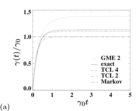
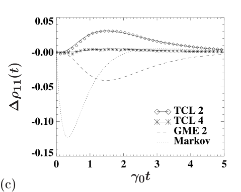
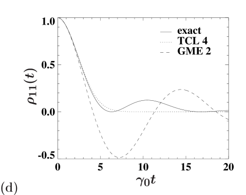
FIG. 1.: The damped Jaynes-Cummings model on resonance. Exact solution (exact), time-convolutionless master equation to second (TCL 2) and fourth order (TCL 4), generalized master equation to second order (GME 2), and the Markovian quantum master equation (Markov): (a) Decay rate of the excited state population, (b) the population of the excited state, including a stochastic simulation of the time-convolutionless quantum master equation with $10^{5}$ realizations, and (c) deviation of the approximative solutions from the exact result, for $\tau_{\rm S}=5\tau_{\rm R}$ (moderate coupling). (d) Population of the excited state for $\tau_{\rm S}=0.2\tau_{\rm R}$ (strong coupling).

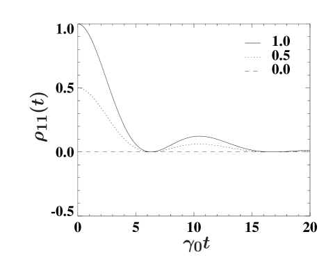
FIG. 2.: The damped Jaynes-Cummings model on resonance. Exact population for the three different initial conditions $\rho_{11}(0)=1.0$, $0.5$, $0.0$ in the strong coupling regime ($\tau_{\rm S}=0.2\tau_{\rm R}$).

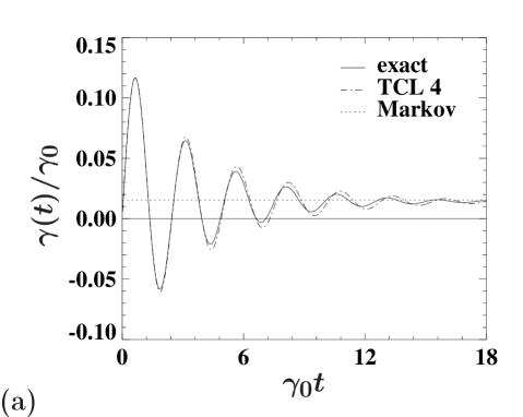
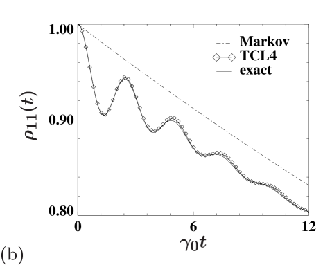
FIG. 3.: The damped Jaynes-Cummings model with detuning. Exact solution (exact), time-convolutionless master equation to fourth order (TCL 4), and the Markovian quantum master equation (Markovian): (a) Decay rate of the excited state population, and (b) the population of the excited state, including a stochastic simulation of the time-convolutionless quantum master equation with $10^{5}$ realizations, for $\lambda=0.3\gamma_{0}$ and $\Delta=8\lambda$

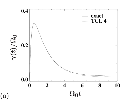
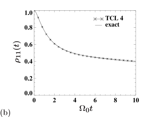
FIG. 4.: Spontaneous decay in a photonic band gap: Exact solution (exact), and time-convolutionless master equation to fourth order (TCL 4): (a) Decay rate of the excited state population, and (b) the population of the excited state, including a stochastic simulation of the time-convolutionless quantum master equation with $10^{5}$ realizations, for $W_{1}=1.1$, $W_{2}=0.1$, $\Gamma_{1}/\Omega_{0}=10$, and $\Gamma_{2}/\Omega_{0}=1$.

REFERENCES

- [1] H. Carmichael, An Open Systems Approach to Quantum Optics, Lecture Notes in Physics m18 (Springer-Verlag, Berlin, Heidelberg, New York, 1993).
- [2] J. Dalibard, Y. Castin, and K. Mølmer, Phys. Rev. Lett. 68, 580 (1992).
- [3] C. W. Gardiner, A. S. Parkins, and P. Zoller, Phys. Rev. A 46, 4363 (1992).
- [4] R. Dum, A. S. Parkins, P. Zoller, and C. W. Gardiner, Phys. Rev. A 46, 4382 (1992).
- [5] N. Gisin and I. C. Percival, J. Phys. A 25, 5677 (1992).
- [6] N. Gisin and I. C. Percival, J. Phys. A 26, 2233 (1993).
- [7] H. M. Wiseman and G. J. Milburn, Phys. Rev. A 47, 1652 (1993).
- [8] H. P. Breuer and F. Petruccione, Fortschr. Phys. 45, 39 (1997).
- [9] Y. Castin and K. Mølmer, Phys. Rev. Lett. 74, 3772 (1995).
- [10] H. P. Breuer, W. Huber, and F. Petruccione, Computer Physics Communications 104, 46 (1997).
- [11] A. Imamoglu, Phys. Rev. A 50, 3650 (1994).
- [12] M. W. Jack, M. J. Collett, and D. F. Walls, quant-ph/9807028 (1998).
- [13] L. Diósi and W. T. Strunz, Phys. Lett. A 235, 569 (1997).
- [14] L. Diósi, N. Gisin and W. T. Strunz, Phys. Rev. A 58, 1699 (1998).
- [15] S. Chaturvedi and J. Shibata, Z. Physik B 35, 297 (1979).
- [16] N. H. F. Shibata, Y. Takahashi, J. Stat. Phys 17, 171 (1977).
- [17] W. Louisell, Quantum Statistical Properties of Radiation (Wiley, New York, 1990).
- [18] C. W. Gardiner, Quantum Noise (Springer-Verlag, New York, 1991).
- [19] N. G. van Kampen, Physica 74, 215 (1974).
- [20] N. G. van Kampen, Stochastic Processes in Physics and Chemistry (North-Holland, Amsterdam, 1981).
- [21] S. Nakajima, Prog. Theor. Phys 20, 948 (1958).
- [22] R. Zwanzig, J. Chem. Phys 33, 1338 (1960).
- [23] P. Résibois, Physica 27, 721 (1963).
- [24] N. G. van Kampen, Physica 74, 239 (1974).
- [25] G. Lindblad, Commun. Math. Phys. 48, 119 (1976).
- [26] H. P. Breuer and F. Petruccione, Phys. Rev. Lett. 74, 3788 (1995).
- [27] H. P. Breuer and F. Petruccione, Phys. Rev. E 52, 428 (1995).
- [28] H. P. Breuer, B. Kappler, and F. Petruccione, Phys. Rev. A 56, 2334 (1997).
- [29] H. P. Breuer, B. Kappler, and F. Petruccione, Eur. Phys. J. D 1, 9 (1998).
- [30] B. M. Garraway, Phys. Rev. A 55, 2290 (1997).
- [31] B. M. Garraway, Phys. Rev. A 55, 4636 (1997).