On the Curvature of Monotone Metrics and a
Conjecture Concerning the Kubo-Mori Metric

Abstract

Monotone metrics on the space of positive matrices generalize the classical Fisher metric of statistical distinguishability of probability distributions to the quantum case. These metrics are in one to one correspondence with operator monotone functions. It is the aim of this article to determine curvature quantities of an arbitrary Riemannian monotone metric using the Riesz-Dunford operator calculus as the main technical tool. The resulting scalar curvature is explained in more detail for three examples. In particular, we show an important conjecture of Petz concerning the Kubo-Mori metric up to a formal proof of the concavity of a certain function on ${\mathbb{R}}_{+}^{3}$. This concavity seems to be numerically evident. The conjecture asserts that the scalar curvature of the Kubo-Mori metric increases if one goes to more mixed states.

I Introduction

Let ${\cal D}_{n}$ resp. ${\cal D}_{n}^{1}$ denote the manifold of complex positive $n\times n$-matrices (of trace one). A Riemannian metric on ${\cal D}_{n}^{1}$ is called monotone if it is decreasing under stochastic mappings (the exact definition is given below). These metrics are of interest in quantum statistics and information theory since ${\cal D}_{n}^{1}$ is the space of (faithful) states (represented by positive density matrices) of an $n$-level quantum system. Monotone metrics generalize the Fisher information (metric) of classical statistics,[5, 8], to the quantum case. Indeed, the restrictions of any monotone metric to the submanifold of diagonal matrices (probability distributions on an $n$-point set) equals (up to a factor) the Fisher metric. Roughly speaking, the Fisher metric measures the statistical distinguishability of probability distributions and a similar meaning is expected in the quantum case, see e.g. [14, 16, 19, 20]. Monotone metrics can be seen as the Hessian of entropy-like functions. The relation between entropies, monotone metrics and operator monotone functions has been considered in several articles , see [24] and references found there. Moreover, in [22] it has been explained how monotone metrics appear on the background of the concept of purification of mixed states [10]. There monotone metrics arise from the reduction of certain metrics on the space of pure states of a larger quantum system. The underlying geometry is that of a Riemannian submersion, [7], where the metric in the purifying space is built by the natural modular operator of the Tomita-Takesaki theory.

A monotone metric of special interest for mathematical and physical reasons, [14, 19, 20, 21, 22], is the so called Bures metric introduced by Uhlmann, [12]. Its curvature quantities are known, [13, 23]. Moreover, certain curvature results were obtained for the Kubo-Mori metric in [15]. It is the first aim of this paper to obtain similar results for the general case (Propositions 1-4). These considerations are based on a classification result of Petz, [17]. Continuing the work of Morozova and Chentsov, [9], who initiated the study of monotone metrics, he proved a one to one correspondence between monotone metrics and operator monotone functions (cf. [2, 3]). Thus, a monotone metric is of the form

$$g_{\varrho}(X,Y)={\rm Tr\,}X^{*}c({\bf L}_{\varrho},{\bf R}_{\varrho})(Y)\,.$$

For calculating curvature quantities we have to handle derivatives with respect to $\varrho$ of the function $c$ of the operators of left and right multiplication. For this purpose we use the Riesz-Dunford operator calculus and obtain the Riemannian curvature tensor for an arbitrary monotone metric. Several authors called objects similar to $c({\bf L},{\bf R})$ superoperators due to the dependence on $\varrho$. We regard $c({\bf L},{\bf R})$ as a field of operators acting on a bundle in order to reflect the underlying geometry.

Special interest we focus on the scalar curvature. The main technical difficulty here is due to the large number of terms one meets. However, we end up with a suitable expression (Theorem 1) for the scalar curvature and apply this result to three examples, the Bures, the largest and the Kubo-Mori metric (Theorem 2). In the last case there is a conjecture of Petz,[15], that the scalar curvature increases if one goes to more mixed states. It is the second aim of this paper to reduce the proof of this important conjecture to the concavity of a certain function on ${\mathbb{R}}_{+}^{3}$ (Theorem 3). This concavity seems to be numerically evident by many experiences and several function plots, although we do not have a formal proof up to now. Since the function in question, $h_{\rm s}$, see formula (77), is homogeneous the asserted concavity is, actually, a certain property of the function $h_{\rm s}(x,y,1)$ in two variables. Of course, this property is stronger than concavity.

The paper is organized as follows. In Section II we fix the framework of the Riesz-Dunford calculus for our purposes. Section III gives the basic definition and classification theorem for monotone metrics and contains some preliminary remarks on Morozova-Chentsov functions. In Sections IV and V we determine the curvature quantities including the examples. Finally, Section VI deals with the monotonicity conjecture.

Notations: Let ${\cal M}_{n}({\mathbb{C}})$ denote the space of complex $n{\times}n$-matrices and ${\cal D}_{n}$ (resp. ${\cal D}_{n}^{1}$) the manifold of positive definite complex matrices $\varrho$ (of trace one). ${\cal D}_{n}^{(1)}$ is an open subset of the space of Hermitian matrices (of trace one). Therefore, we identify the tangent spaces ${\rm T}_{\varrho}{\cal D}_{n}^{(1)}$ of these manifolds in an obvious way with the space of Hermitian (traceless for ${\cal D}_{n}^{1}$) matrices and consider vector fields $\cal X,Y,\dots$ as functions on ${\cal D}_{n}^{(1)}$ with values in these vector spaces. By the corresponding italic symbols we mean vectors tangent at $\varrho$ resp. the values of a vector field at $\varrho$, $X={\cal X}_{\varrho}$, etc. for the fixed point $\varrho$ we have in mind. $[{\cal X,Y}]$ is understood as the commutator of these matrix valued functions, i.e. $[{\cal X,Y]_{\varrho}:=\cal X_{\varrho}Y_{\varrho}-\cal X_{\varrho}Y_{\varrho}}=[X,Y]$, whereas the usual commutator of vector fields is denoted by $[{\cal X,Y}]_{\rm vf}$. By ${\bf L}_{\varrho}$ and ${\bf R}_{\varrho}$ we denote the operators of left resp. right multiplication by $\varrho\in{\cal D}_{n}^{(1)}$. Therefore, ${\bf L}$ and ${\bf R}$ are fields of operators. But, similarly to other geometrical object, we frequently omit the index $\varrho$ for simplicity of notation even if we have a concrete point $\varrho$ in mind. Moreover, if $\bf L$ or $\bf R$ are indicated otherwise we mean the corresponding multiplication operators.

II Operator Calculus

Let $f$ be a complex analytic function defined on a neighborhood of ${\mathbb{R}}_{+}$. Then we have by the Riesz-Dunford operator calculus

$$f(\varrho)=\frac{1}{2\pi{\bf i}}\oint f(\xi)(\xi-\varrho)^{-1}\,{\rm d}\xi\,,$$

where $\xi(t)$ is a path surrounding the positive spectrum of $\varrho$. For a diagonal $\varrho$ this is just Cauchy’ integral formula applied to each eigenvalue. We notice, that the operators ${\bf L}_{\varrho}$ and ${\bf R}_{\varrho}$ are selfadjoint w.r. to the Hermitian form $X,Y\mapsto{\rm Tr\,X^{*}\,Y}$ on ${\cal M}_{n}({\mathbb{C}})$ and their common spectrum equals the spectrum of $\varrho$ (with multiplicity $n$). Thus, the function $f$ of the operator ${\bf L}_{\varrho}$, $f\left({\bf L}_{\varrho}\right)$, is well defined and has, again by the Riesz-Dunford calculus, the representation

$$f\left({\bf L}_{\varrho}\right)=\frac{1}{2\pi{\bf i}}\oint f(\xi)\left(\xi{\bf Id}-{\bf L}_{\varrho}\right)^{-1}\,{\rm d}\xi\,.$$ (1)

Since left and right multiplication commute a similar reasoning applies to a function $c$, complex analytic in two variables, of ${\bf L}_{\varrho}$ and ${\bf R}_{\varrho}$. This results in

$$c({\bf L}_{\varrho},{\bf R}_{\varrho})=\frac{1}{(2\pi{\bf i})^{2}}\oint\!\!\oint c(\xi,\eta)\frac{1}{\xi{\bf Id}-{\bf L}_{\varrho}}\circ\frac{1}{\eta{\bf Id}-{\bf R}_{\varrho}}\,{\rm d}\xi\,{\rm d}\eta\,$$ (2)

or, equivalently,

$$c({\bf L}_{\varrho},{\bf R}_{\varrho})(Y)=\frac{1}{(2\pi{\bf i})^{2}}\oint\!\!\oint c(\xi,\eta)\frac{1}{\xi-\varrho}Y\frac{1}{\eta-\varrho}\,{\rm d}\xi\,{\rm d}\eta\,,$$ (3)

where we integrate in every variable once around the spectrum of $\varrho$. These integral formulae are the main technical tool for what follows, because they allow for determining derivatives of functions of $\varrho$, $\bf L$ and $\bf R$, e.g.

$$\frac{\rm d}{{\rm d}t}f\left(\varrho+tX\right)_{|t=0} = \frac{1}{2\pi{\bf i}}\oint f(\xi)\frac{1}{\xi-\varrho}\,X\,\frac{1}{\xi-\varrho}\,{\rm d}\xi$$

$$\frac{\rm d}{{\rm d}t}f\left({\bf L}_{\varrho+tX}\right)_{|t=0} = \frac{1}{2\pi{\bf i}}\oint f(\xi)\frac{1}{\xi{\bf Id}-{\bf L}_{\varrho}}\circ{\bf L}_{X}\circ\frac{1}{\xi{\bf Id}-{\bf L}_{\varrho}}\,{\rm d}\xi\,,\qquad X=X^{*}\in{\rm T}_{\varrho}{\cal D}_{n}\subset{\cal M}_{n}({\mathbb{C}}).$$

The last expression is just the covariant derivative of $f({\bf L})$ in the direction $X$ w.r. to the local flat affine structure on ${\cal D}$ inherited from $\left\{M\in{\cal M}_{n}({\mathbb{C}})|M=M^{*}\right\}$. We denote this flat covariant derivative by ${\rm D}$. The derivative ${\rm D}_{\!X}c({\bf L},{\bf R})$ and the second order derivatives which we need later on are obtained similarly from (2) or (3) applying the Leibniz rule to the composition of resolvents. Since these formulae are obvious, we do not write down them here.

The right hand sides of the last two equations become more explicit if we decompose the tangent vector as $X=Y+[A,\varrho]$, where $[Y,\varrho]=Y\varrho-\varrho Y=0$ and $A=-A^{*}$ (The existence of such a decomposition can be seen assuming that $\varrho$ is diagonal). Now a simple calculation yields

$$\frac{\rm d}{{\rm d}t}f\left(\varrho+tX\right)_{|t=0}=Yf^{\prime}(\varrho)+[A,f(\varrho)]$$

$${\rm D}_{\!X}f({\bf L})_{\varrho} = \frac{\rm d}{{\rm d}t}f\left({\bf L}_{\varrho+tX}\right)_{|t=0}={\bf L}_{Y}\circ f^{\prime}({\bf L}_{\varrho})+\left[{\bf L}_{A},{\bf L}_{f(\varrho)}\right]={\bf L}_{Yf^{\prime}(\varrho)+[A,f(\varrho)]}\,.$$

But, in order to remove integrals in the forthcoming second order derivatives we would have to consider more subtle decompositions. Moreover, the functions $c$ we regard are of the form $1/(f(s/t)t)$, so that, actually, one needs only one integration to consider $f(\bf L_{\varrho}/\bf R_{\varrho})$. In [11] a calculus for its first order derivatives has been developed, which leads for diagonal $\varrho$, essentially, to a Pick matrix method found in [2], Chap. VIII. However, here we need the second order derivatives as well, and we will not try to avoid the integrals. The approach used here has the advantage of symmetry.

III Monotone Metrics

A family of Riemannian metrics $g=\left\{g^{n}\right\}$ on $\left\{{\cal D}_{n}^{1}\right\}$, ${n\in{\mathbb{N}}}$, is called monotone iff

$$g^{m}_{{\bf T}(\varrho)}({\bf T}_{*}(X),{\bf T}_{*}(X))\leq g^{n}_{\varrho}(X,X)$$

holds for every stochastic mapping ${\bf T}:{\cal M}_{n}({\mathbb{C}})\rightarrow{\cal M}_{m}({\mathbb{C}})$ and all $\varrho\in{\cal D}_{n}^{1}$, $X\in{\rm T}_{\varrho}{\cal D}_{n}^{1}$. For more details we refer to [17], where Petz considered, roughly speaking, monotone Hermitian forms on the complexified tangent bundles of ${\cal D}_{n}^{1}$. The above defined monotone Riemannian metrics in [17] are called symmetric monotone metrics and the real part of a monotone Hermitian form is, of course, symmetric. We will use a slightly different terminology. By a monotone metric we will always mean a monotone Riemannian metrics, since we are interested here only in those ones. From now on we fix an integer $n\geq 2$ and omit the index $n$ at $g^{n}$ and ${\cal D}_{n}^{(1)}$. Thus, we mean by $g$ either the whole family or the concrete metric related to the number $n$ we have in mind.

Theorem [17]: There is a one to one correspondence between monotone Riemannian metrics $g$ and operator monotone functions $f:{\mathbb{R}}_{+}\rightarrow{\mathbb{R}}_{+}$ satisfying the symmetry condition $f(t)=t\,f(1/t)$. This correspondence is given by

$$g_{\varrho}(X,Y)={\rm Tr}\,X\frac{1}{f({\bf L}_{\varrho}/{\bf R}_{\varrho}){\bf R}_{\varrho}}(Y)\,,\qquad X,Y\in{\rm T}_{\varrho}{\cal D}^{1}.$$

For the definition, integral representation and main properties of operator monotone functions we refer to [2, 3]. A crucial point for what follows is the fact, that such a function has a complex analytic extension to the open right complex half plane such that $f(\overline{x})=\overline{f(x)}$. Thus, the function c defined by

$$c(x,y):=\frac{1}{f(x/y)y}\,,$$ (4)

called the Morozova-Chentsov function related to the monotone metric $g$, is analytic in both arguments on an open neighborhood of ${\mathbb{R}}_{+}^{\;2}\subset{\mathbb{C}}^{2}$ and the metric $g$ takes the more appropriate for our purposes form

$$g({\cal X},{\cal Y})={\rm Tr}\,{\cal X}\,c({\bf L},{\bf R})({\cal Y})\,,$$ (5)

or, equivalently,

$$g_{\varrho}(X,Y)=\frac{1}{(2\pi{\bf i})^{2}}\,{\rm Tr}\oint\!\!\oint c(\xi,\eta)X(\xi-\varrho)^{-1}Y(\eta-\varrho)^{-1}\,\,{\rm d}\xi\,{\rm d}\eta\,.$$ (6)

Clearly, the above formulae also define a Riemannian metric on ${\cal D}$, which we also denote by $g$. In the next sections we will first deal with this manifold and then consider ${\cal D}^{1}$ as a Riemannian submanifold of codimension 1.

Some examples of symmetric operator monotone functions are

$$f(x)=\frac{x+1}{2}\,,\quad\frac{2x}{x+1}\,,\quad\frac{x-1}{\ln x}$$

leading to the Morozova-Chentsov functions

$$c(x,y)=\frac{2}{x+y}\,,\quad\frac{x+y}{2xy}\,,\quad\frac{\ln x-\ln y}{x-y}$$ (7)

and to the smallest, largest and Kubo-Mori metric. For further examples we refer to [3, 17]. For the time being we are interested in the general case and return to these examples later.

The calculations of the following sections make use of certain algebraic and differential properties common for all Morozova-Chentsov functions. Multiplying a monotone metric by a factor if necessary, we will assume from now on that the corresponding operator monotone function $f$ is normalized by $f(1)=1$. This and the above mentioned properties of $f$ imply

$$c(x,x)=\frac{1}{x}$$ (8)

$$c(\overline{x},\overline{y})=\overline{c(x,y)}\,,\qquad c(x,y)=c(y,x)\,,\qquad c(x,y)=t\;c(t\,x,t\,y)\,,\quad t\in{\mathbb{R}}_{+}\,.$$ (9)

Lets denote by $c^{(k,l)}$ the partial derivatives of $c$ of order $(k,l)$. Then we have by the symmetry of $c$

$$c^{(k,l)}(x,y)=c^{(l,k)}(y,x)$$ (10)

and differentiating the last equation of (9) w.r. to $t$ and $x,y$ yields the further identities

$$c(x,y)+x\,c^{(1,0)}(x,y)+y\,c^{(0,1)}(x,y) = 0$$ (11)

$$2\,c^{(1,0)}(x,y)+y\,c^{(1,1)}(x,y)+x\,c^{(2,0)}(x,y) = 0$$ (12)

$$2\,c^{(0,1)}(x,y)+x\,c^{(1,1)}(x,y)+y\,c^{(0,2)}(x,y) = 0\,.$$ (13)

In particular,

$$c^{(1,0)}(x,x)=c^{(0,1)}(x,x)=-\frac{1}{2x^{2}},$$ (14)

but there is no such identity for $c^{(2,0)}(x,x)$, cf. (7).

We will have to do with partial derivatives of order at most two. Thus we can always remove the mixed derivatives $c^{(1,1)}$ and replace $c^{(0,k)}$ by $c^{(k,0)}$ changing the order of arguments. For simplicity we write $c^{\prime}$ and $c^{\prime\prime}$ instead of $c^{(1,0)},c^{(2,0)}$. Exhausting the above relations we can attain that $c^{(k,0)}$, $k\leq 2$, has arguments ordered alphabetically. This uniqueness is useful for comparing expressions, however, we will not always insist on such an ordering, since it may destroy the symmetry. Therefore, we leave it at the reduced equations (12)

$$c(x,y)+x\,c^{\prime}(x,y)+y\,c^{\prime}(y,x) = 0\,$$ (15)

$$2x\,c^{\prime}(x,y)+x^{2}c^{\prime\prime}(x,y) = 2y\,c^{\prime}(y,x)+y^{2}c^{\prime\prime}(y,x)\,.$$ (16)

Finally, it will be convenient to use partial logarithmic derivatives instead of usual ones and we apply the above notation to the function $\ln c$ too,

$$(\ln c)^{\prime}(x,y):=\frac{\partial\ln c(x,y)}{\partial x}=\frac{c^{\prime}(x,y)}{c(x,y)}\,.$$ (17)

For example, the first identity of (12) now reads

$$1+x\,(\ln c)^{\prime}(x,y)+y\,(\ln c)^{\prime}(y,x)=0\,.$$

IV Covariant Derivative and Curvature Tensor

A Not Normalized Case

As already mentioned in Section II the manifold $\cal D$ carries locally a natural flat affine structure related to the usual parallel displacement. The corresponding covariant derivative ${\rm D}$ is the derivation along straight lines, i.e.

$$({\rm D}_{\!Z}{\cal T})_{\varrho}=\frac{{\rm d}}{{\rm d}t}\,{{\cal T}_{\varrho+t\,Z}}_{\restriction t=0}\,,\qquad Z\in{\rm T}_{\varrho}{\cal D}\,,$$ (18)

for any tensor field $\cal T$ on $\cal D$. In particular

$${\rm D}_{Z}{\varrho}=Z\,.$$ (19)

Since the trace and the matrix multiplication are compatible with this flat affine structure the Leibniz rule implies

$${\rm D}_{\!Z}(\xi-\varrho)^{-1}=(\xi-\varrho)^{-1}Z\,(\xi-\varrho)^{-1}\,,\qquad\xi\in{\mathbb{C}}\,.$$ (20)

From (3) we obtain for the flat covariant derivative of $c({\bf L},{\bf R})$

$${\rm D}_{\!Z}c({\bf L},{\bf R})_{\varrho}\;(Y)=\frac{1}{(2\pi{\bf i})^{2}}\oint\!\!\oint c(\xi,\eta)\left\{\frac{1}{\xi-\varrho}Z\frac{1}{\xi-\varrho}Y\frac{1}{\eta-\varrho}+\frac{1}{\xi-\varrho}Y\frac{1}{\eta-\varrho}Z\frac{1}{\eta-\varrho}\right\}\,{\rm d}\xi\,{\rm d}\eta\,,$$ (21)

and, therefore, using (5)

$${\rm D}_{\!Z}g\;(X,Y)=\frac{1}{(2\pi{\bf i})^{2}}\,{\rm Tr}\oint\!\!\oint c(\xi,\eta)\,Z\,\left\{\frac{1}{\xi-\varrho}\,X\,\frac{1}{\eta-\varrho}\,Y\,\frac{1}{\xi-\varrho}+\frac{1}{\xi-\varrho}\,Y\,\frac{1}{\eta-\varrho}\,X\,\frac{1}{\xi-\varrho}\right\}\,{\rm d}\xi\,{\rm d}\eta\,.$$ (22)

Similarly we proceed we the flat derivative of second order with respect to vector fields $\cal X$ and $\cal Y$. We denote it by ${{\rm D}}^{2}_{\!\cal X,Y}$, i.e.

$${{\rm D}}^{2}_{\!\cal X,Y}:={\rm D}_{\!\cal X}{\rm D}_{\cal Y}-{\rm D}_{{\rm D}_{\!\cal X}\cal Y}.$$

Clearly the differential operator ${{\rm D}}^{2}_{\!\cal X,Y}$ at $\varrho$ depends only on the values of the fields at this point, cf. [7].

From (22) we find using the Leibniz rule

$${{\rm D}}^{2}_{\!Z,W}\!g\;(X,Y) = \frac{1}{(2\pi{\bf i})^{2}}\,{\rm Tr}\oint\!\!\oint c(\xi,\eta)\,\left\{\left(Z\frac{1}{\xi-\varrho}W+W\frac{1}{\xi-\varrho}Z\right)\frac{1}{\xi-\varrho}X\frac{1}{\eta-\varrho}Y\frac{1}{\xi-\varrho}\right.$$ (24)

$$\hskip 99.58464pt+\left.Z\frac{1}{\xi-\varrho}X\frac{1}{\eta-\varrho}W\frac{1}{\eta-\varrho}Y\frac{1}{\xi-\varrho}\right\}{\rm d}\xi\,{\rm d}\eta+\{X\leftrightarrow Y\}\,.$$

The symbol $\{X\leftrightarrow Y\}$ means the expression before with exchanged $X$ and $Y$.

Now let $\nabla$ be the covariant derivative related to the Levi-Civit connection of the metric $g$. It is uniquely determined by

$$2g(\nabla_{\!\cal X}{\cal Y},{\cal Z})={\cal X}g({\cal Y},{\cal Z})+{\cal Y}g({\cal X},{\cal Z})-{\cal Z}g({\cal X},{\cal Y})+g([{\cal X},{\cal Y}]_{\rm vf},{\cal Z})+g([{\cal Z},{\cal X}]_{\rm vf},{\cal Y})+g({\cal X},[{\cal Z},{\cal Y}]_{\rm vf})\,.$$

Moreover, $\nabla_{\!\cal X}{\cal Y}$ is of the form

$$\nabla_{\!\cal X}{\cal Y}={\rm D}_{\!{\cal X}}{\cal Y}+\Gamma({\cal X,Y})\,,$$ (25)

where $\Gamma$ is a certain symmetric (1,2)-tensor field on $\cal D$, because every two torsionless covariant derivatives are related in this way. In an affine coordinate system on $\cal D$ it would be described by the usual Christoffel symbols $\Gamma_{i,j}^{k}$. This allows us to use the symbol $\Gamma$, although, in general the Christoffel symbols are not of tensorial type. Now the above defining equation turns out to be equivalent to the requirement that

$$2g(\Gamma({X,Y}),{Z})={\rm D}_{\!X}g\;({Y,Z})+{\rm D}_{Y}g\;({X,Z})-{\rm D}_{\!Z}g\;({X,Y})$$ (26)

holds for all tangent vectors $X,Y,Z$. This corresponds to the formulae for the Christoffel symbols in terms of the coefficients of the metric tensor and their first order derivatives.

Proposition 1: Let $X=X^{*},Y=Y^{*}\in{\rm T}_{\varrho}{\cal D}$, then

$$\Gamma(X,Y)=$$ (27)

$$\frac{1}{2(2\pi{\bf i})^{2}c({\bf L},{\bf R})}\oint\!\!\oint c(\xi,\eta)\left\{\frac{1}{\xi{-}\varrho}X\frac{1}{\xi{-}\varrho}Y\frac{1}{\eta{-}\varrho}+\frac{1}{\eta{-}\varrho}X\frac{1}{\xi{-}\varrho}Y\frac{1}{\xi{-}\varrho}-\frac{1}{\xi{-}\varrho}X\frac{1}{\eta{-}\varrho}Y\frac{1}{\xi{-}\varrho}\right\}{\rm d}\xi{\rm d}\eta+\{X\leftrightarrow Y\}$$ (28)

Proof: The right hand side of (28) is Hermitian by (9), i.e. it is a vector tangent to $\cal D$. Using (22) one verifies straightforwardly that (28) fulfills (26), where one can assume for brevity of calculation that $Y=X$. $\Box$

Next we consider the Riemannian curvature tensor given by

$${\cal R}({\cal X,Y,Z,W}):=g\left({\cal X},\nabla_{\!\cal Z}\nabla_{\!\cal W}{\cal Y}-\nabla_{\!\cal W}\nabla_{\!\cal Z}{\cal Y}-\nabla_{[{\cal Z,W}]_{\rm vf}}{\cal Y}\right)\,.$$ (29)

It can be expressed in terms of $\Gamma$ and ${\rm D}^{2}g$, indeed we show:

Proposition 2:

$${\cal R}({\cal X,Y,Z,W}) = g(\Gamma(X,W),\Gamma(Y,Z))-g(\Gamma(X,Z),\Gamma(Y,W))$$ (31)

$$+\frac{1}{2}\left({{\rm D}}^{2}_{\!{\cal X,W}}g\;({\cal Y,Z})+{{\rm D}}^{2}_{{\cal Y,Z}}g\;({\cal X,W})-{{\rm D}}^{2}_{{\cal X,Z}}g\;({\cal Y,W})-{{\rm D}}^{2}_{{\cal Y,W}}g\;({\cal X,Z})\right)\,,$$

where ${{\rm D}}^{2}g$ and $\Gamma$ are given by (24) and (28).

Proof: Actually (31) corresponds to the known formula for the coefficients of the curvature tensor in terms of Christoffel symbols and second order derivatives of the metric coefficients w.r. to a coordinate system. Thus we derive (31) from (29) not appealing to the particular metric we have in mind. In order to simplify this calculation let us assume for the moment that $\cal X,Y,Z$ and $\cal W$ are parallel vector fields w.r. to the underlying flat affine structure, i.e. they are constant Hermitian matrix valued functions. Then the flat derivative ${\rm D}_{\!\cal X}{\cal Y}$ and the commutator $[{\cal X,Y}]_{\rm vf}={\rm D}_{\!\cal X}{\cal Y}-{\rm D}_{\!\cal Y}{\cal X}$ vanish for all pairs of these fields and ${{\rm D}}^{2}_{\!\cal X,Y}={\rm D}_{\!\cal X}{\rm D}_{\!\cal Y}={\rm D}_{\!\cal Y}{\rm D}_{\!\cal X}$. Thus we get using $\nabla g=0$ and (25)

$${\cal R}({\cal X,Y,Z,W}) = g\left({\cal X},\nabla_{\!\cal Z}\nabla_{\!\cal W}{\cal Y}-\nabla_{\!\cal W}\nabla_{\!\cal Z}{\cal Y}\right)$$

$$= \nabla_{\!\cal Z}\left(g({\cal X},\nabla_{\!\cal W}{\cal Y})\right)-g(\nabla_{\!\cal Z}{\cal X},\nabla_{\!\cal W}{\cal Y})-\nabla_{\!\cal W}\left(g({\cal X},\nabla_{\!\cal Z}{\cal Y})\right)+g(\nabla_{\!\cal W}{\cal X},\nabla_{\!\cal Z}{\cal Y})$$

$$= g(\Gamma({\cal X,W}),\Gamma({\cal Y,Z}))-g(\Gamma({\cal X,Z}),\Gamma({\cal Y,W}))$$

$$+{\cal Z}\left(g({\cal X},\Gamma({\cal Y,W}))\right)-{\cal W}\left(g({\cal X},\Gamma({\cal Y,Z}))\right)\,.$$

But the last two terms yield by (26)

$$\frac{1}{2}{\rm D}_{\!\cal Z}\left\{{\rm D}_{\!\cal Y}g\;({\cal X,W})+{\rm D}_{\cal W}g\;({\cal X,Y})-{\rm D}_{\!\cal X}g\;({\cal Y,W})\right\}-\frac{1}{2}{\rm D}_{\cal W}\left\{{\rm D}_{\cal Y}g\;({\cal X,Z})+{\rm D}_{\!\cal Z}g\;({\cal X,Y})-{\rm D}_{\!\cal X}g\;({\cal Y,Z})\right\}$$

$$= \frac{1}{2}\left({{\rm D}}^{2}_{\!\cal X,W}g\;({\cal Y,Z)}+{{\rm D}}^{2}_{\!\cal Y,Z}g\;({\cal X,W)}-{\rm D}^{2}_{\!\cal X,Z}g\;({\cal Y,W})-{{\rm D}}^{2}_{\cal Y,W}g\;({\cal X,Z)}\right)\,.$$

$\Box$

B Normalized Case

The knowledge of the covariant derivative and the curvature of $({\cal D},g)$ allows for determining these quantities for the codimension one submanifold $({\cal D}^{1},g)$. We denote them by ${}^{1}\nabla$ and ${\cal R}^{1}$. For this purpose let $\cal X,Y\dots$ be vector fields on ${\cal D}^{1}$ extended to some neighborhood of ${\cal D}^{1}$ in ${\cal D}$.

First of all we observe that the radial vector field $\cal N$ given by

$${\cal N}_{\varrho}:=\varrho\,,\qquad\varrho\in{\cal D}\,,$$ (32)

is perpendicular to all submanifolds of positive matrices with fixed trace, in particular to ${\cal D}^{1}$. Indeed, let $X\in{\rm T}_{\varrho}{\cal D}$ with ${\rm Tr\,}X=0$, then

$$g(X,\varrho)={\rm Tr\,}{X}\,c({\bf L}_{\varrho},{\bf R}_{\varrho})(\varrho)={\rm Tr}\,X\,c(\varrho,\varrho)\varrho={\rm Tr}\,X\,\varrho^{-1}\varrho={\rm Tr}\,X=0\,,$$

where we used $c(x,x)=1/x$, see (8). Moreover, this field is normalized at ${\cal D}^{1}$, $g({\cal N,N})_{\varrho}=g_{\varrho}(\varrho,\varrho)={\rm Tr\,}\varrho=1$ and satisfies

$${\rm D}_{\cal X}{\cal N}={\cal X}$$ (33)

for all vector fields $\cal X$ on $\cal D$. Actually, this is a more precise formulation of (19). The following relations concerning this radial field are less obvious.

Lemma 1: For all vector fields $\cal X,Y,Z$ on $\cal D$ holds

$${\rm i)} \Gamma({\cal X,N})=-\frac{1}{2}\,X$$ (34)

$${\rm ii)} g(\Gamma({\cal X,Y}),{\cal N})=-\frac{1}{2}\,g({\cal X,Y})$$ (35)

$${\rm iii)} {\cal R(X,Y,Z,N})=0$$ (36)

Proof:

i) From (28) and (12) we get

$$\Gamma({\cal X,N})_{\varrho} = \frac{1}{2(2\pi{\bf i})^{2}c({\bf L},{\bf R})}\oint\!\!\oint c(\xi,\eta)\left\{\frac{\varrho}{(\xi{-}\varrho)^{2}}X\frac{1}{\eta-\varrho}+\frac{1}{\xi-\varrho}X\frac{\varrho}{(\eta-\varrho)^{2}}\right\}{\rm d}\xi{\rm d}\eta$$

$$= \frac{1}{2\,c({\bf L},{\bf R})}\left({\bf L}_{\varrho}\circ c^{(1,0)}({\bf L}_{\varrho},{\bf R}_{\varrho})+{\bf R}_{\varrho}\circ c^{(0,1)}({\bf L}_{\varrho},{\bf R}_{\varrho})\right)(X)=-\frac{1}{2}\,X\,.$$

ii) By the symmetry it is sufficient to prove the assertion for ${\cal X}={\cal Y}$. From (26) and i) we conclude

$$g(\Gamma({\cal X,X}),{\cal N}) = {\rm D}_{\cal X}g\;({\cal X,N})-\frac{1}{2}\,{\rm D}_{\cal N}g\;({\cal X,X})={\rm D}_{\cal X}g\;({\cal X,N})-g({\cal X},\Gamma({\cal X,N}))$$

$$= {\rm D}_{\cal X}(g({\cal X,N}))-g({\rm D}_{\cal X}{\cal X},{\cal N})-g({\cal X},{\rm D}_{\cal X}{\cal N})+\frac{1}{2}\,g({\cal X,X})$$

$$= {\rm D}_{\cal X}({\rm Tr\,}{\cal X})-{\rm Tr\,}{\rm D}_{\cal X}{\cal X}-g({\cal X,X})+\frac{1}{2}\,g({\cal X,X})=-\frac{1}{2}\,g({\cal X,X})$$

iii) From (33) and i) we infer $\nabla_{\cal X}{\cal N}={\rm D}_{\cal X}{\cal N}+\Gamma({\cal X},{\cal N})={\cal X}/2$ and the last assertion follows since the torsion of $\nabla$ vanishes.

$$2{\cal R(X,Y,Z,N})=2{\cal R(Z,N,X,Y})=2g\left({\cal Z,\left(\nabla_{X}\nabla_{Y}-\nabla_{Y}\nabla_{X}-\nabla_{[X,Y]_{\rm vf}}\right)N}\right)=g\left({\cal Z},{\cal\nabla_{X}Y-}{\cal\nabla_{Y}X-}{\cal\,[X,Y]_{\rm vf}}\right)=0$$

$\Box$

Now, let $\cal X,Y$ be tangent vector fields on ${\cal D}^{1}$ extended to some neighborhood of ${\cal D}^{1}$ in ${\cal D}$, $g_{\varrho}({\cal X,N})=0$ for $\varrho\in{\cal D}^{1}$. Then ${}^{1}\!\nabla_{\!\cal X}{\cal Y}$ is the component of $\nabla_{\!\cal X}{\cal Y}$, tangent to ${\cal D}^{1}$, [1], i.e.

$${}^{1}\!\nabla_{\!\cal X}{\cal Y}=\nabla_{\!\cal X}{\cal Y}-g({\cal N},\nabla_{\!\cal X}{\cal Y}){\cal N}\,.$$

Since ${\cal D}^{1}$ is a (locally) affine subspace of ${\cal D}$ the derivative ${\rm D}_{\!\cal X}{\cal Y}$ is tangent to ${\cal D}^{1}$ and we conclude from (25) and (35)

Proposition 3:

$${}^{1}\!\nabla_{\!\cal X}{\cal Y}={\rm D}_{\!\cal X}{\cal Y}+\Gamma({\cal X,Y})+\frac{1}{2}\,g({\cal X,Y})\,{\cal N}\,,$$ (37)

where $\Gamma$ is given by Proposition 1. $\Box$

Thus, the component of $\nabla_{\cal\!X}{\cal Y}$ normal to ${\cal D}^{1}$ equals $-g({\cal X,Y}){\cal N}/2$ and we obtain the curvature tensor ${\cal R}^{1}$ of the submanifold ${\cal D}^{1}$ by the Gauss equation, [1]:

Proposition 4:

$${\cal R}^{1}({\cal X,Y,Z,W})={\cal R}({\cal X,Y,Z,W})+\frac{1}{4}(g({\cal X,Z})g({\cal Y,W})-g({\cal Y,Z})g({\cal X,W}))\,,$$ (38)

where $\cal R$ is given by Proposition 3. $\Box$

V scalar Curvature

A General Theorem

The scalar curvature at $\varrho\in{\cal D}^{(1)}$ we denote by $\cal S_{\varrho}$ resp. ${\cal S}_{\varrho}^{1}$. It is given by

$${\cal S}_{\varrho}^{(1)}=\sum_{X\neq Y\in{\cal B}^{(1)}}{\cal K}^{(1)}(X,Y)\,,$$ (39)

where we sum up over pairs of different elements of an orthogonal basis ${\cal B}^{(1)}$ of ${\rm T}_{\varrho}{\cal D}^{(1)}$. The sectional curvature of the plane generated by orthogonal vectors $X$ and $Y$ equals due to Propositions 2 and 4

$${\cal K}^{(1)}(X,Y)=\frac{1}{g(X,X)g(Y,Y)}{\cal R}(X,Y,X,Y)\quad+\quad\left(\;\frac{1}{4}\;\right)\,,$$ (40)

where

$${\cal R}(X,Y,X,Y) = g(\Gamma(X,Y),\Gamma(X,Y))-g(\Gamma(X,X),\Gamma(Y,Y))$$ (42)

$$+{{\rm D}}^{2}_{\!X,Y}g\;(X,Y)-\frac{1}{2}{{\rm D}}^{2}_{X,X}g\;(Y,Y)-\frac{1}{2}{{\rm D}}^{2}_{Y,Y}g\;(X,X)\,.$$

It turns out that ${\cal S}^{1}$ and ${\cal S}$ differ at $\varrho\in{\cal D}^{1}$ only by a constant depending on $n$. Indeed, let the basis ${\cal B}$ consists of the normal vector ${\cal N}_{\varrho}=\varrho$ and a certain basis ${\cal B}^{1}$ of ${\rm T}_{\varrho}{\cal D}^{1}$. Then by Lemma 1 the normal vector does not give any contribution to $\cal S$ in (39). Since ${\cal S}^{1}$ is a sum of $2\left({n^{2}-1\atop 2}\right)$ terms we get

Corollary 1: Let $\varrho\in{\cal D}^{1}$. Then

$${\cal S}_{\varrho}^{1}={\cal S}_{\varrho}+\frac{(n^{2}-1)(n^{2}-2)}{4}\,.$$ (43)

$\Box$

Thus it is sufficient to consider the not normalized case. In order to formulate our theorem we introduce the functions $h_{1},\dots,h_{4}$ complex analytic in every argument in a certain neighborhood of ${\mathbb{R}}_{+}^{\;3}\subset{\mathbb{C}}^{3}$. We define them for different arguments by

$$h_{1}(x,y,z) = \frac{c(x,y)-z\,c(x,z)\,c(y,z)}{(x-z)(y-z)c(x,z)c(y,z)}$$ (44)

$$h_{2}(x,y,z) = \frac{\left(c(x,z)-c(y,z)\right)^{2}}{(x-y)^{2}c(x,y)c(x,z)c(y,z)}$$ (45)

$$h_{3}(x,y,z) = z\,\frac{(\ln c)^{\prime}(z,x)-(\ln c)^{\prime}(z,y)}{x-y}$$ (46)

$$h_{4}(x,y,z) = z\,(\ln c)^{\prime}(z,x)\;(\ln c)^{\prime}(z,y)\,,$$ (47)

otherwise we go to the limit, $h_{1}(x,x,z):=\lim_{y\rightarrow x}h_{1}(x,y,z)$ etc. Indeed, using the general properties (8)-(17) of the Morozova-Chentsov function $c$ one easily verifies, that all these limits exist. By Riemann’ theorem about removable singularities the resulting functions are in fact complex analytic in every argument. A similar reasoning applies to other functions in this section involving so called divided differences.

For simplicity of notation we consider the spectrum $\sigma(\varrho)$ as an $n$-tuple with possibly repeated elements if some eigenvalues appear with multiplicities, but, nevertheless, we write $x\in\sigma(\varrho)$. Thus, e.g. $\sum_{x\neq y\in\sigma(\varrho)}term(x,y)$ always means a sum over $n^{2}-n$ pairs of eigenvalues, also if some or all eigenvalues numerically coincide. Hence, this sum is equivalent to the more extensive expression $\sum_{i\neq j=1,\dots,n}term(\lambda_{i},\lambda_{j})$. A similar reasoning applies to other sums with one or three indices of summation. In the following summations the indices $x,y,z$ run through the spectrum in this sense and $i,j,k$ through $1,\dots,n$. This convention enables us to formulate the main theorem of this section.

Theorem 1: The scalar curvature on the manifold $({\cal D},g)$ of $n\times n$ positive matrices equals

$${\cal S}_{\varrho} = \sum_{x,y,z\in\sigma(\varrho)}h(x,y,z)-\sum_{x\in\sigma(\varrho)}h(x,x,x)\,,\qquad\mbox{where}$$ (48)

$$h(x,y,z) := h_{1}(x,y,z)-\frac{1}{2}h_{2}(x,y,z)+2h_{3}(x,y,z)-h_{4}(x,y,z)\,.$$ (49)

Before we prove the Theorem we give some conclusions and remarks.

First of all, there is some ambiguity in the choice of the function $h$. Indeed, we can replace $h$ by any function with the same symmetrization not changing the sum. In particular we can replace $h$ by its symmetrization $h_{\rm s}$,

$$h_{\rm s}(x,y,z):=\frac{1}{3}\left(h(x,y,z)+h(y,z,x)+h(z,x,y)\right)\,.$$ (50)

In the above Theorem we tried to find a certain minimal formulation with different types of divided differences, so that the involved functions have no singularities if arguments coincide. However, for a concrete function $c$ another representation could be more convenient (see the examples below).

Going to the limit in (44)-(47) results in

$$h(x,x,x)=\frac{15}{8x}-3x^{2}\,c^{\prime\prime}(x,x)\,.$$ (51)

Moreover, we see that (48) is, actually, a trace formula. Indeed, we can look at (48) as a trace of functions of $\varrho$, that means

$${\cal S}_{\varrho} = {\rm Tr\,}\left\{\left({\rm Tr\,}\left\{\left({\rm Tr\,}h(s,t,\varrho)\right)_{|t=\varrho}\right\}\right)_{|s=\varrho}\right\}+{\rm Tr\,}\left\{-\frac{15}{8}\varrho^{-1}+3\varrho^{2}c^{\prime\prime}(\varrho,\varrho)\right\}\,.$$

Thus, the scalar curvature can equal well be written as a threefold complex integral around the spectrum of $\varrho$.

Corollary 2:

$${\cal S}_{\varrho} = \oint\!\!\oint\!\!\oint h(\xi,\eta,\tau)\,{\rm Tr\,}\frac{1}{\xi-\varrho}\,{\rm Tr\,}\frac{1}{\eta-\varrho}\,{\rm Tr\,}\frac{1}{\tau-\varrho}\,{\rm d}\xi\,{\rm d}\eta\,{\rm d}\tau+{\rm Tr\,}\left\{-\frac{15}{8}\varrho^{-1}+3\varrho^{2}c^{\prime\prime}(\varrho,\varrho)\right\}\,.$$ (52)

$\Box$

A further consequence concerns the curvature at the most mixed state of ${\cal D}^{1}$. For $\varrho=\frac{1}{n}\mathchoice{{\hbox{\boldmath$\displaystyle 1$}}}{{\hbox{\boldmath$\textstyle 1$}}}{{\hbox{\boldmath$\scriptstyle 1$}}}{{\hbox{\boldmath$\scriptscriptstyle 1$}}}$ we obtain

$${\cal S}^{1}_{\varrho}=(n^{3}-n)\,h(1{/}n,1{/}n,1{/}n)+\frac{(n^{2}-1)(n^{2}-2)}{4}$$

leading to

Corollary 3: The scalar curvature on ${\cal D}^{1}$ at $\varrho=\frac{1}{n}{\mathchoice{{\hbox{\boldmath$\displaystyle 1$}}}{{\hbox{\boldmath$\textstyle 1$}}}{{\hbox{\boldmath$\scriptstyle 1$}}}{{\hbox{\boldmath$\scriptscriptstyle 1$}}}}$ equals

$${\cal S}^{1}_{\varrho}=\frac{(n^{2}-1)(17n^{3}-4n-24\,c^{\prime\prime}(1/n,1/n))}{8n}\,.$$ (53)

In particular, in the case of the smallest, largest and Kubo-Mori metric related to the Morozova-Chentsov functions (7) holds

$${\cal S}^{1}_{\varrho}=\frac{(n^{2}-1)(5n^{2}-4)}{8}\,,\quad\frac{(1-n^{2})(7n^{2}+4)}{8}\,\;\mbox{ resp. }\frac{(n^{2}-1)(n^{2}-4)}{8}\,.$$

$\Box$
This confirms the result obtained for the Kubo-Mori metric at $\varrho=\frac{1}{n}{\mathchoice{{\hbox{\boldmath$\displaystyle 1$}}}{{\hbox{\boldmath$\textstyle 1$}}}{{\hbox{\boldmath$\scriptstyle 1$}}}{{\hbox{\boldmath$\scriptscriptstyle 1$}}}}$ in [15], Theorem 6.2. For the minimal metric this coincides with Corollary 3 of [23]. The differing factor is due to a factor $1/4$ in the metric.

Finally, let ${\cal S}(\lambda_{1},\dots,\lambda_{n}):={\cal S}_{\varrho}$, where $\lambda_{i}$ are the eigenvalues of $\varrho$. Then, using $h_{\rm s}$ instead of $h$, it is not difficult to verify, that the following recurrences hold

Corollary 4:

$$(n-3)\,{\cal S}(\lambda_{1},\dots,\lambda_{n}) = \sum_{i}{\cal S}(\lambda_{1},\dots,{}^{\stackrel{{\scriptstyle\displaystyle{i}}}{{\vee}}},\dots,\lambda_{n})-\sum_{i<j}{\cal S}(\lambda_{i},\lambda_{j})\,,$$ (54)

$${\cal S}(\lambda_{1},\dots,\lambda_{n}) = \sum_{i<j<k}{\cal S}(\lambda_{i},\lambda_{j},\lambda_{k})-(n-3)\sum_{i<j}{\cal S}(\lambda_{i},\lambda_{j})\,,\qquad n>3$$ (55)

$\Box$

Proof of Theorem 1: Since the metric is invariant under the ${\rm U}(n)$-conjugation on $\cal D$ we fix a diagonal $\varrho$ with the spectrum $\sigma(\varrho):=\left\{\lambda_{1},\dots,\lambda_{n}\right\}$. We set

$${\rm b}_{ij}:={\rm e}_{ij}+{\rm e}_{ji}\qquad\mbox{and}\qquad\widetilde{\rm b}_{ij}:={\bf i\,}({\rm e}_{ij}-{\rm e}_{ji})\,,$$

where ${\rm e}_{ij}$, $i,j=1,\dots,n$, are the standard matrices with entries zero or one. Then

$${\cal B}:=\left\{{\rm b}_{ii}|1\leq i\leq n\right\}\cup\left\{{\rm b}_{ij}|1\leq i<j\leq n\right\}\cup\left\{\widetilde{\rm b}_{ij}|1\leq i<j\leq n\right\}$$

is an orthogonal basis and in the sum (39) there appear terms of, essentially, three types, say A, B and C. To see this, we first observe that the sectional curvature vanishes for pairs of basis vectors with disjoint index sets, because ${\cal K}(b,b^{\prime})$ is built, finally, by products of diagonal resolvent matrices and $b,b,b^{\prime},b^{\prime}$ (cf. (24) and (28)). By the same reason ${\cal K}(b,b^{\prime})$ depends only on the eigenvalues corresponding to the indices involved. Moreover, using the U$(n)$-invariance immediately follows

$${\cal K}({\rm b}_{ii},{\rm b}_{ij})={\cal K}({\rm b}_{ii},\widetilde{\rm b}_{ij})\,\qquad{\cal K}({\rm b}_{ik},{\rm b}_{jk})={\cal K}({\rm b}_{ik},\widetilde{\rm b}_{jk})={\cal K}(\widetilde{\rm b}_{ik},\widetilde{\rm b}_{jk})\,\quad\mbox{for }i\neq j\neq k\neq i\,,$$

because the arguments of $\cal K$ generate conjugated planes. For example, in the case of the second equation let ${\rm U}={\rm diag}(\dots,1,\dots,{\bf i},\dots,1,\dots)$ with $\bf i$ in the $j$-th position. Then ${\rm U}\varrho{\rm U}^{*}=\varrho$, ${\rm U}{\rm b}_{ik}{\rm U}^{*}={\rm b}_{ik}$ and ${\rm U}{\rm b}_{jk}{\rm U}^{*}=\widetilde{\rm b}_{jk}$. The other identities follow by a similar choice of U.

Thus, all non vanishing terms in the sum (39) are equal to one of the expressions ${\cal K}({\rm b}_{ii},{\rm b}_{ij})$, ${\cal K}({\rm b}_{ij},\widetilde{\rm b}_{ij})$ or ${\cal K}({\rm b}_{ik},{\rm b}_{jk})$, which can be obtained from ${\cal K}({\rm b}_{11},{\rm b}_{12})$, ${\cal K}({\rm b}_{12},\widetilde{\rm b}_{12})$ and ${\cal K}({\rm b}_{13},{\rm b}_{23})$ by changing the indices at $\lambda$. Hence, the knowledge of the dependence of these three terms on $\lambda_{1},\lambda_{2}$ resp. $\lambda_{1},\lambda_{2},\lambda_{3}$ allows for determining (39). Let this dependence be given by the three functions $A$, $B$ and $C$, that means

$$A(x,y):={\cal K}({\rm b}_{11},{\rm b}_{12})\,,\quad B(x,y):={\cal K}({\rm b}_{12},\widetilde{\rm b}_{12})\,,\quad C(x,y,z):={\cal K}({\rm b}_{13},{\rm b}_{23})\,,$$ (56)

where we assume on the right hand sides that the eigenvalues $\lambda_{1},\lambda_{2},\lambda_{3}$ equal the independent variables $x,y,z$. Of course, $B$ and $C$ are symmetric in $x,y$.

The computation of $A$, $B$ and $C$ requires many straightforward calculations based on Propositions 1 and 2. We do not present them in full details and explain only some essential intermediate results for $B$. For a detailed verification the use of Mathematica or a similar program is suggested. Moreover, the function $A$ we can obtain from $C$ as we will see in Lemma 3.

Lemma 2:

$$B(x,y) = {{2-(x+y)\,c(x,y)}\over{{{\left(x-y\right)}^{2}}\,c(x,y)}}-\frac{x\,(\ln c)^{\prime}(x,y)^{2}}{4}-\frac{y\,(\ln c)^{\prime}(y,x)^{2}}{4}-\frac{x\,(\ln c)^{\prime}(x,y)-y\,(\ln c)^{\prime}(y,x)}{x-y}$$ (57)

$$C(x,y,z) = \frac{1}{4}\left(3h_{1}(x,y,z)-h_{1}(y,z,x)-h_{1}(z,x,y)\right)$$ (58)

$$+ \frac{1}{8}\left(h_{2}(x,y,z)+h_{2}(y,z,x)+h_{2}(z,x,y)\right)-\frac{h_{4}(x,y,z)}{4}$$ (59)

$$+ \left\{\left(\frac{c(z,y)-c(x,y)}{2(x-z)^{2}c(x,z)\,c(y,z)}+\frac{z\,(\ln c)^{\prime}(z,y)}{2(x-z)}\right)+\{x\leftrightarrow y\}\right\}$$ (60)

Proof: According to (56) we set $n=2$, $\lambda_{1}=x$, $\lambda_{2}=y$ and

$$\varrho:=\left(\begin{array}[]{cc}x&0\\ 0&y\end{array}\right)\,,\quad X:={\rm b}_{11}=2{\rm e}_{11}=\left(\begin{array}[]{cc}2&0\\ 0&0\end{array}\right)\,,\quad Y:={\rm b}_{12}={\rm e}_{12}+{\rm e}_{21}=\left(\begin{array}[]{cc}0&1\\ 1&0\end{array}\right)\,;\quad X,Y\in{\rm T}_{\varrho}{\cal D}\,.$$

Equation (5) yields $g(X,X)=4c(x,x)=4/x$ and $g(Y,Y)=2c(x,y)$. Further, using Proposition 1 we find

$$\Gamma(X,X) = \frac{1}{(2\pi{\bf i})^{2}}\oint\!\!\oint\frac{2c(\xi,\eta)}{(\xi-x)^{2}(\eta-x)}\,{\rm d}\xi\,{\rm d}\eta\;\,c({\bf L},{\bf R})^{-1}(X)=-\frac{1}{x}\,X$$

$$\Gamma(X,Y) = \frac{1}{(2\pi{\bf i})^{2}}\oint\!\!\oint\frac{c(\xi,\eta)}{(\xi-x)^{2}(\eta-y)}\,{\rm d}\xi\,{\rm d}\eta\;\,c({\bf L},{\bf R})^{-1}(Y)=(\ln c)^{\prime}(x,y)\,Y$$

$$\Gamma(Y,Y) = \frac{1}{(2\pi{\bf i})^{2}}\oint\!\!\oint\left\{\frac{2c(\xi,\eta)}{(\xi-x)(\xi-y)(\eta-x)}-\frac{c(\xi,\eta)}{(\xi-x)^{2}(\eta-y)}\right\}\,{\rm d}\xi\,{\rm d}\eta\;\,c({\bf L},{\bf R})^{-1}({\rm e}_{11})$$

$$+ \frac{1}{(2\pi{\bf i})^{2}}\oint\!\!\oint\left\{\frac{2c(\xi,\eta)}{(\xi-x)(\xi-y)(\eta-y)}-\frac{c(\xi,\eta)}{(\xi-y)^{2}(\eta-x)}\right\}\,{\rm d}\xi\,{\rm d}\eta\;\,c({\bf L},{\bf R})^{-1}({\rm e}_{22})$$

$$= \left(\frac{2(1-x\,c(x,y))}{x-y}-x\,c^{\prime}(x,y)\right)\,{\rm e}_{11}+\left(\frac{2(1-y\,c(x,y))}{y-x}-y\,c^{\prime}(y,x)\right)\,{\rm e}_{22}$$

and, therefore,

$$g(\Gamma(X,Y),\Gamma(X,Y)) = \frac{2\,c^{\prime}(x,y)^{2}}{c(x,y)}$$

$$-g(\Gamma(X,X),\Gamma(Y,Y)) = \frac{4(1-x\,c(x,y))}{x^{2}(x-y)}-\frac{2\,c^{\prime}(x,y)}{x}\,.$$

For the second order derivatives we obtain from (24)

$$-\frac{1}{2}{\rm D}_{\!X,X}g\;(Y,Y) = -\frac{1}{(2\pi{\bf i})^{2}}\oint\!\!\oint\frac{8\,c(\xi,\eta)}{(\xi-x)^{3}(\eta-y)}\,{\rm d}\xi\,{\rm d}\eta=-4\,c^{\prime\prime}(x,y)$$

$${\rm D}_{\!X,Y}g\;(X,Y)-\frac{1}{2}{\rm D}_{Y,Y}g\;(X,X) = \frac{1}{(2\pi{\bf i})^{2}}\oint\!\!\oint\frac{8\,c(\xi,\eta)}{(\xi-x)^{2}(\eta-x)(\eta-y)}\,{\rm d}\xi\,{\rm d}\eta=\frac{4(1+2x^{2}c^{\prime}(x,y))}{x^{2}(y-x)}$$

Inserting all that into (40), (42) and (56) finishes the proof of (57). The treatment of $C$ is analogous, however it needs much more numerical effort. $\Box$

Lemma 3:

$${\rm i)} \qquad A(x,y)=2C(x,y,x)$$ (61)

$${\rm ii)} \qquad B(x,y)=2C(x,x,y)+2C(y,y,x)$$ (62)

Proof: We set $n=3$, $\lambda_{1}=\lambda_{3}=x$, $\lambda_{2}=y$, $X={\rm b}_{13}$ and $Y={\rm b}_{23}$. Then $g({\rm b}_{11},{\rm b}_{11})=|\!|{\rm b}_{11}|\!|^{2}=|\!|{\rm b}_{33}|\!|^{2}=4/x$, $|\!|X|\!|^{2}=2/x$, $|\!|{\rm b}_{12}|\!|^{2}=|\!|Y|\!|^{2}=2c(x,y)$ and

$$A(x,y) = {\cal K}_{\varrho}({\rm b}_{11},{\rm b}_{12})=\frac{x}{8c(x,y)}\,{\cal R}({\rm b}_{11},{\rm b}_{12},{\rm b}_{11},{\rm b}_{12})\,,$$

$$C(x,y,x) = {\cal K}_{\varrho}({\rm b}_{13},{\rm b}_{23})=\frac{x}{4c(x,y)}\,{\cal R}({\rm b}_{13},{\rm b}_{23},{\rm b}_{13},{\rm b}_{23})={\cal K}_{\varrho}(X,Y)\,.$$

Now we use the ${\rm U}(3)$-symmetry of conjugation. For this purpose let

$$u:=\left(\begin{array}[]{ccc}\sqrt{2}/2&0&\sqrt{2}/2\\ 0&1&0\\ \sqrt{2}/2&0&-\sqrt{2}/2\end{array}\right)\in{\rm U}(3)\,.$$

Then $u\varrho u^{*}=\varrho$ and ${\cal R}_{\varrho}(X,Y,X,Y)={\cal R}_{\varrho}(X^{\prime},Y,X^{\prime},Y^{\prime})$ with $X^{\prime}:=uXu^{*}=\left({\rm b}_{11}-{\rm b}_{33}\right)/2$ and $Y^{\prime}=uYu^{*}=\sqrt{2}\left({\rm b}_{12}-{\rm b}_{23}\right)/2$. Thus,

$$C(x,y,x) = {\cal K}(X,Y)=\frac{x}{4c(x,y)}{\cal R}_{\varrho}(X^{\prime},Y^{\prime},X^{\prime},Y^{\prime})=\frac{x}{4c(x,y)}\frac{1}{8}{\cal R}({\rm b}_{11}{-}{\rm b}_{33},{\rm b}_{12}-{\rm b}_{23},{\rm b}_{11}{-}{\rm b}_{33},{\rm b}_{12}-{\rm b}_{23})$$

$$= \frac{x}{32c(x,y)}\big{\{}{\cal R}({\rm b}_{11},{\rm b}_{12},{\rm b}_{11},{\rm b}_{12})+{\cal R}({\rm b}_{33},{\rm b}_{23},{\rm b}_{33},{\rm b}_{23})+\dots\big{\}}$$

$$= \frac{x}{32c(x,y)}\big{\{}|\!|{\rm b}_{11}|\!|^{2}\,|\!|{\rm b}_{12}|\!|^{2}\,A(x,y)+{|\!|\rm b}_{33}|\!|^{2}\,|\!|{\rm b}_{23}|\!|^{2}\,A(x,y)\big{\}}=\frac{1}{2}\,A(x,y)\,.$$

All the terms indicated by dots in the above equation vanish. From (31), (28) and (24) we see that these terms are built by products of the four arguments of the curvature tensor and resolvents. Now, considering the indices of the arguments of the neglected terms it is not difficult to see, that these products (e.g. for ${\cal R}({\rm b}_{11},{\rm b}_{12},{\rm b}_{33},{\rm b}_{12})$), or at least their traces (e.g. ${\cal R}({\rm b}_{11},{\rm b}_{12},{\rm b}_{11},{\rm b}_{23})$), vanish. This finishes the proof of (61).

To prove (62) we give $C(x,x,y)$ resulting from (60). Then (62) is immediately verified.

$$C(x,x,y) = \lim_{z\rightarrow x}C(x,z,y)$$ (63)

$$= \frac{2-(x+y)\,c(x,y)}{4\,(x-y)^{2}\,c(x,y)}+\frac{x\,(\ln c)^{\prime}(x,y)^{2}}{8}-\frac{y\,(\ln c)^{\prime}(y,x)^{2}}{4}-\frac{x\,(\ln c)^{\prime}(x,y)-y\,(\ln c)^{\prime}(y,x)}{4\,(x-y)}$$ (64)

$\Box$

Now we can proceed with the computation of $\cal S_{\varrho}$ starting with (39),

$${\cal S}_{\varrho} = 4\sum_{i\neq j}{\cal K}({\rm b}_{ii},{\rm b}_{ij})+2\sum_{i\neq j}{\cal K}({\rm b}_{ij},\widetilde{\rm b}_{ij})+4\!\!\!\sum_{\textstyle{i<j\,;\,k<l\atop(i,j)\neq(k,l)}}{\cal K}({\rm b}_{ij},{\rm b}_{kl})$$

$$= \sum_{x\neq y}\Big{\{}4A(x,y)+B(x,y)\Big{\}}+4\sum_{x\neq y\neq z\neq x}C(x,y,z)$$

$$= 4\sum_{x,y,z}C(x,y,z)+\sum_{x}\Big{\{}-4A(x,x)-B(x,x)+8C(x,x,x)\Big{\}}$$

$$+\sum_{x,y}\Big{\{}4A(x,y)+B(x,y)-4C(x,x,y)-8C(x,y,x)\Big{\}}$$

$$= 4\sum_{x,y,z}C(x,y,z)-4\sum_{x}C(x,x,x)\,,$$

where we used Lemma 3 and $\sum_{x,y}2C(x,x,y)=\sum_{x,y}\left(C(x,x,y)+C(y,y,x)\right)$. Next, inserting (60) yields

$${\cal S}_{\varrho} = 4\sum_{x,y,z}\left\{\frac{1}{4}\,h_{1}(x,y,z)+\frac{3}{8}\,h_{2}(x,y,z)-\frac{1}{4}\,h_{4}(x,y,z)+\frac{c(z,y)-c(x,y)}{(x-z)^{2}c(x,z)\,c(y,z)}+\frac{z\,(\ln c)^{\prime}(z,y)}{(x-z)}\right\}$$

$$-4\sum_{x}C(x,x,x)\,.$$

The two fractions, whose sum has no singularities, we replace by $-h_{2}(x,y,z)/2$ and $h_{3}(x,y,z)/2$, which have the same symmetrizations as the replaced terms. We end up with

$${\cal S}_{\varrho}=\sum_{x,y,z}\left\{h_{1}(x,y,z)-\frac{1}{2}\,h_{2}(x,y,z)+2\,h_{3}(x,y,z)-h_{4}(x,y,z)\right\}-4\sum_{x}C(x,x,x)=\sum_{x,y,z}h(x,y,z)-\sum_{x}h(x,x,x)\,$$

where we used $4C(x,x,x)=h(x,x,x)$, since $4C$ and $h$ have the same symmetrization. This finishes the proof of Theorem 1. $\Box$

B Examples

In this paragraph we consider the scalar curvature for three important examples of monotone metrics related to the Morozova-Chentsov functions (7) given in Section III.

1 The smallest monotone metric, $c(x,y)=\frac{2}{x+y}$

This metric was first introduced by Uhlmann in generalizing the Berry phase to mixed states, [12]. Now it is often called Bures metric, since it is, roughly speaking, the infinitesimal version of the Bures distance of mixed quantum states. It appears very natural in the concept of purifications of mixed states and intertwines between the classical Fisher metric and the Study-Fubini metric on the complex projective space representing pure states of a quantum system. There are many papers dealing with this metric. Some references where given in the Introduction, for curvature results see [13, 23]. Nevertheless we explain this example, at least to see, that the whole machinery presented here works.

Equations (44)-(47) yield for $c(x,y)=\frac{2}{x+y}$

$$h_{1}(x,y,z)=\frac{1}{2(x+y)}\,,\qquad h_{2}(x,y,z)=\frac{x+y}{2(x+z)(y+z)}\,,\qquad h_{3}(x,y,z)=h_{4}(x,y,z)=\frac{z}{(x+z)(y+z)}$$

Thus, by Theorem 1 the scalar curvature of $\cal D$ at $\varrho$ equals

$${\cal S}_{\varrho} = \sum_{x,y,z}h(x,y,z)-\sum_{x}h(x,x,x)=\sum_{x,y,z}\left\{\frac{1}{2(x+y)}-\frac{x+y}{4(x+z)(y+z)}+\frac{z}{(x+z)(y+z)}\right\}-\frac{3}{8}\sum_{x}\frac{1}{x}$$

$$= \sum_{x,y,z}\left\{\frac{1}{4(x+z)}+\frac{1}{4(y+z)}-\frac{x+y}{4(x+z)(y+z)}+\frac{z}{(x+z)(y+z)}\right\}-\frac{3}{8}\sum_{x}\frac{1}{x}$$

Thus

$${\cal S}_{\varrho}=\frac{3}{2}\sum_{x,y,z}\frac{z}{(x+z)(y+z)}--\frac{3}{8}\sum_{x}\frac{1}{x}\,,$$

where we sum up over the spectrum of $\varrho$. This confirms the result obtained in [23], where one can find also expressions for the scalar curvature in terms of invariants of $\varrho$. The different factor is due to an other normalization of the metric, as already mentioned above. In particular, we get from Corollary 1 for $n=2$ and $\sigma(\varrho)=\{\lambda_{1},\lambda_{2}\}$, $\lambda_{1}+\lambda_{2}=1$,

$${\cal S}_{\varrho}^{1}=\frac{9}{2(\lambda_{1}+\lambda_{2})}+\frac{3}{2}=6\,$$

i.e. ${\cal D}^{1}$ is a space of constant curvature for this exceptional dimension, In our normalization it looks locally like a sphere of radius 2. This was one of the first results concerning this metric, [12]. For higher dimensions a similar result does not hold, ${\cal D}^{(1)}$ is not a locally symmetric space, [13].

2 The largest monotone metric, $c(x,y)=\frac{x+y}{2\,x\,y}$

This metric belongs to the series of monotone metrics related to

$$c_{s}(x,y):=\frac{x^{2\alpha}+y^{2\alpha}}{2(x\,y)^{\alpha+1/2}}\,,\qquad 0\leq\alpha\leq\frac{1}{2}\,,$$

see [17], also for further references of its application. It is the monotone metric obtained in the simplest way besides the Hilbert-Schmidt metric. Indeed,

$$g_{\varrho}(X,Y)=\frac{1}{2}{\rm Tr\,}X\varrho^{-1}(\varrho\,Y+Y\varrho)\varrho^{-1}=\frac{1}{2}{\rm Tr\,}\varrho^{-1}(XY+YX)$$

and further quantities one can get without using the integral representations, e.g.

$${\rm D}_{\!Z}g\;(X,Y) = -\frac{1}{2}{\rm Tr\,}\varrho^{-1}Z\varrho^{-1}(XY+YX)\,,\qquad{\rm D}^{2}_{\!Z,W}g\;(X,Y)=\frac{1}{2}{\rm Tr\,}\varrho^{-1}(W\varrho^{-1}Z+Z\varrho^{-1}W)\varrho^{-1}(XY+YX)$$

$$\Gamma(X,Y) = \frac{1}{2({\bf L}+{\bf R})}(XY+YX)-\frac{1}{2}(X\varrho^{-1}Y+Y\varrho^{-1}X)\,.$$

Thus, using Proposition 2, it is easy to write down the curvature tensor. For the scalar curvature we rely on our Theorem 1,

$$h_{1}(x,y,z) = h_{3}(x,y,z)=\frac{-z}{(x+z)(y+z)}\,,\qquad h_{2}(x,y,z)=\frac{2z^{2}}{(x+y)(x+z)(y+z)}\,,$$

$$h_{4}(x,y,z) = \frac{xy}{z(x+z)(y+z)}\,,\qquad h(x,x,x)=\frac{-9}{8x}\,,$$

and proceed with

$${\cal S}_{\varrho} = \sum_{x,y,z}(h_{1}+2h_{3})(x,y,z)-\frac{1}{2}\sum_{x,y,z}h_{2}(x,y,z)-\sum_{x,y,z}h_{4}(x,y,z)-\sum_{x}h(x,x,x)$$

$$= -3\sum_{x,y,z}\frac{z}{(x+z)(y+z)}-\sum_{x,y,z}\left(\frac{x}{(x+z)(y+z)}-\frac{z}{2(x+z)(y+z)}\right)-\sum_{x,y,z}\frac{x\,y}{z(x+z)(y+z)}+\sum_{x}\frac{9}{8x}$$

$$= -\frac{5}{2}\sum_{z}z\,\left(\sum_{x}\frac{1}{x+z}\right)^{2}-\sum_{z}\left(\sum_{x}\frac{x}{x+z}\right)\left(\sum_{x}\frac{1}{x+z}\right)-\sum_{z}\frac{1}{z}\left(\sum_{x}\frac{x}{x+z}\right)^{2}+\sum_{x}\frac{9}{8x}$$

$$= -\frac{5}{2}\sum_{z}z\,\left(\sum_{x}\frac{1}{x+z}\right)^{2}+n\sum_{x,z}\frac{1}{x+z}+\left(\frac{9}{8}-n^{2}\right)\sum_{x}\frac{1}{x}\,.$$

Inserting

$$\sum_{x}\frac{1}{x+t}={\rm Tr\,}\frac{1}{\varrho+t}=-\frac{\chi^{\prime}(-t)}{\chi(-t)}\,,$$

where $\chi(t):=\sum e_{n-i}(-t)^{i}$ is the characteristic polynomial of $\varrho$, we get the scalar curvature as a trace of a function of $\varrho$ (diagonal or not):

$${\cal S}_{\varrho}=-\frac{5}{2}{\rm Tr\,}\varrho\,\frac{\chi^{\prime}(-\varrho)^{2}}{\chi(-\varrho)^{2}}-n\,{\rm Tr\,}\frac{\chi^{\prime}(-\varrho)}{\chi(-\varrho)}+\left(\frac{9}{8}-n^{2}\right){\rm Tr\,}\varrho^{-1}\,.$$ (65)

Moreover, we can express the scalar curvature in terms of the elementary invariants $e_{i}$. For this purpose we consider the matrix

$${\cal E}_{ij}:=\left\{\begin{array}[]{lll}1&&\mbox{for }i+1=j\\ (-1)^{n-j}e_{n+1-j}&&\mbox{for }i=n\\ 0&&\mbox{otherwise}\end{array}\right.$$

It has the same characteristic polynomial as $\varrho$ and, therefore, it is conjugated (not unitarily) to $\varrho$ in the generic case of different eigenvalues. But the set of $\varrho$ with different eigenvalues is dense in $\cal D$ and by continuity of the scalar curvature we conclude

Proposition 5:

$${\cal S}_{\varrho}=-\frac{5}{2}{\rm Tr\,}{\cal E}\,\frac{\chi^{\prime}(-{\cal E})^{2}}{\chi(-{\cal E})^{2}}-n\,{\rm Tr\,}\frac{\chi^{\prime}(-{\cal E})}{\chi(-{\cal E})}+\left(\frac{9}{8}-n^{2}\right){\rm Tr\,}{\cal E}^{-1}\,.$$ (66)

$\Box$

A similar result was obtained in [23] for the previous example.

3 The Kubo-Mori metric, $c(x,y)=\frac{\log(x)-\log(y)}{x-y}$

This metric was considered by Petz, Hiai and Toth, [15, 17], where they pointed out its importance in information theory and quantum statistics and obtained partial results concerning the sectional and scalar curvature. In [15] the scalar curvature at the trace state, cf. Corollary 3, and the sectional curvature $K_{\varrho}(X,Y)$ where found for $X,Y$ commuting with $\varrho$. Our Theorem 1 leads to a closed expression for the scalar curvature at arbitrary $\varrho$ in terms of its eigenvalues. This result is the basis for the last section, where we consider the conjecture mentioned in the Introduction.

For the functions $h_{i}$ we obtain

$$h_{1}(x,y,z) = h_{3}(x,y,z)=\frac{\displaystyle\frac{z-x+z\,(\ln x-\ln z)}{(x-z)(\ln x-\ln z)}-\frac{z-y+z\,(\ln y-\ln z)}{(y-z)(\ln y-\ln z)}}{x-y}$$

$$h_{2}(x,y,z) = h_{1}(x,y,z)+h_{1}(y,z,x)+h_{1}(z,x,y)$$

$$h_{4}(x,y,z) = \frac{(z-x+z\,(\ln x-\ln z))\;(z-y+z\,(\ln y-\ln z))}{z\,(x-z)(\ln x-\ln z)\;\;\;\;(y-z)(\ln y-\ln z)\;\;}\,,\quad h(x,x,x)=\frac{-1}{8x}\,.$$

We observe, that now $h_{2}$ is already a symmetric function. The typical term seen in these equations is

$$\frac{z-x+z\,(\ln x-\ln z)}{(x-z)(\ln x-\ln z)}=z\,(\ln c)^{\prime}(z,x)$$

and we set

$$d(x,y,z) := \frac{3}{2}h_{1}(x,y,z)-h_{4}(x,y,z)=z\,\left(3\frac{(\ln c)^{\prime}(z,x)-(\ln c)^{\prime}(z,y)}{2(x-y)}-(\ln c)^{\prime}(z,x)\,(\ln c)^{\prime}(z,y)\right)$$ (67)

$$= 3\;\frac{\displaystyle\frac{z-x+z\,(\ln x-\ln z)}{(x-z)(\ln x-\ln z)}-\frac{z-y+z\,(\ln y-\ln z)}{(y-z)(\ln y-\ln z)}}{2(x-y)}-\frac{(z-x+z\,(\ln x-\ln z))\;(z-y+z\,(\ln y-\ln z))}{z\,(x-z)(\ln x-\ln z)\;\;\;\;(y-z)(\ln y-\ln z)\;\;}.$$ (68)

If two arguments coincide the values of $d$ are easily found, we do not list them. Clearly, $d$ has the same symmetrization as $h$ and $h(x,x,x)=d(x,x,x)$. Thus we infer from Corollary 1 and Theorem 1

Theorem 2: The scalar curvature of the Kubo-Mori metric on ${\cal D}^{(1)}$ at $\varrho$ equals

$${\cal S}_{\varrho}^{(1)}=\sum_{x,y,z\in\sigma(\varrho)}d(x,y,z)-\sum_{x\in\sigma(\varrho)}d(x,x,x)\quad\left(\;+\frac{(n^{2}-1)(n^{2}-2)}{4}\;\right)\,.$$ (69)

$\Box$

The following graph of ${\cal S}^{1}$ restricted to the (open) 2-dimensional simplex ($n=3$)

$$\left\{{\rm diag}(\lambda_{1},\lambda_{2},\lambda_{3})\,|\,\lambda_{1}+\lambda_{2}+\lambda_{3}=1\\ \,,\lambda_{i}>0\right\}$$

of diagonal densities will be instructive for the aim of the next section.

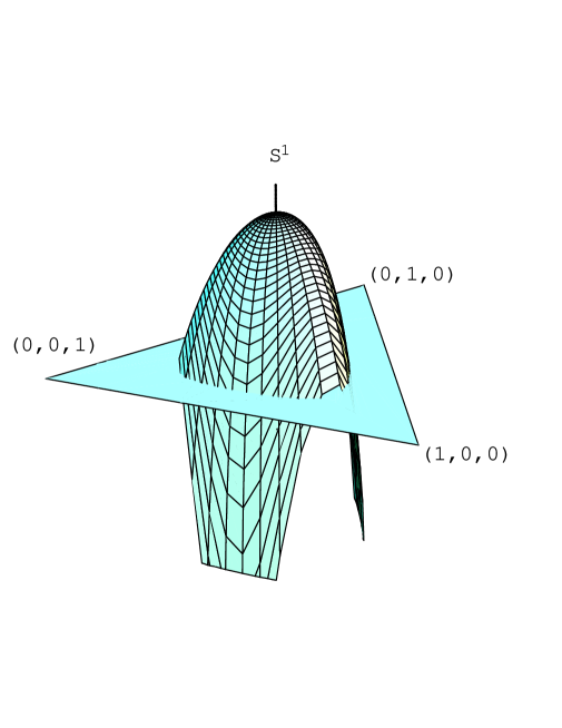
FIG. 1.: Graph of ${\cal S}^{1}$ for $n=3$

Moreover, using this Theorem one confirms all numerical examples given for $n=3$ in [15], however one has to work with high numerical precision if two eigenvalues are close to each other.

It should be mentioned that formula (31) for the curvature simplifies for this metric, because the terms with second order derivatives of $g$ cancel out. Due to general properties of quadrilinear forms (see [1]) this is equivalent to the vanishing of the sum of the corresponding three terms in (42). We do not explain this in detail and refer also to [15], formula (6.4). In our approach one could proceed as follows: Under the additional assumption

$$(y-x)c(y,x)+(x-z)c(x,z)+(z-y)c(z,y)=0$$

for a general Morozova-Chentsov function c one can show

$${\rm D}_{X}g\;(X,Y)={\rm D}_{Y}g\;(X,X)\,.$$

Clearly, this assumption is fulfilled in this example. Now it is not difficult to conclude

$$2{{\rm D}}^{2}_{\!X,Y}g\;(X,Y)-{{\rm D}}^{2}_{X,X}g\;(Y,Y)-{{\rm D}}^{2}_{Y,Y}g\;(X,X)=0\,,$$

and, therefore, (42) reads

$${\cal R}(X,Y,X,Y)=g(\Gamma(X,Y),\Gamma(X,X))-g(\Gamma(X,X),\Gamma(Y,Y))\,.$$ (70)

VI Monotonicity of ${\cal S}^{1}$ under mixing for the Kubo-Mori metric

The manifold ${\cal D}^{1}$ represents the space of faithful mixed states of a $n$-dimensional quantum system and carries the following partial order (for details and further related facts used here we refer e.g. to [4]): $\rho$ is called more mixed than $\varrho$, $\rho\mathchoice{{\hbox{\boldmath$\displaystyle\,\succ\,$}}}{{\hbox{\boldmath$\textstyle\,\succ\,$}}}{{\hbox{\boldmath$\scriptstyle\,\succ\,$}}}{{\hbox{\boldmath$\scriptscriptstyle\,\succ\,$}}}\varrho$, if there exists a trace preserving stochastic map $\alpha$ such that $\rho=\alpha(\varrho)$. If $\lambda_{i},\mu_{i}$ are the eigenvalues of $\rho$ and $\varrho$ in decreasing order this relation becomes equivalent to

$$\lambda_{1}+\dots+\lambda_{k}\leq\mu_{1}+\dots+\mu_{k},\qquad k=1,\dots,n\,.$$

Petz conjectured that the scalar curvature of the Kubo-Mori metric on ${\cal D}^{1}$ behaves monotonously under this partial order, more precisely:

Conjecture, [15, 18] :

$$\rho\mathchoice{{\hbox{\boldmath$\displaystyle\,\succ\,$}}}{{\hbox{\boldmath$\textstyle\,\succ\,$}}}{{\hbox{\boldmath$\scriptstyle\,\succ\,$}}}{{\hbox{\boldmath$\scriptscriptstyle\,\succ\,$}}}\varrho\quad\Longrightarrow\quad{\cal S}^{1}_{\rho}\geq{\cal S}^{1}_{\varrho}$$ (71)

An immediate consequence would be that the scalar curvature on ${\cal D}^{1}$ attains its maximum at the most mixed state, i.e. at the trace state. Hence, $\max{\cal S}^{1}={\cal S}^{1}_{\mathchoice{{\hbox{\boldmath$\displaystyle 1$}}}{{\hbox{\boldmath$\textstyle 1$}}}{{\hbox{\boldmath$\scriptstyle 1$}}}{{\hbox{\boldmath$\scriptscriptstyle 1$}}}/n}=(n^{2}-1)(n^{2}-4)/8$, see Corollary 3.

In this section we shows this important conjecture up to the concavity of a certain function in three variables, respectively up to some weaker consequences of this concavity. For this purpose we use the results for the Kubo-Mori metric obtained in the example before.

Since the scalar curvature is invariant under U$(n)$ conjugation, it is sufficient to consider the conjecture on the $(n-1)$-dimensional (open) simplex $\left\{{\rm diag}(\lambda_{1},\dots,\lambda_{n})|\sum\lambda_{i}=1\,,\lambda_{i}>0\right\}$. Clearly, FIG. 1 supports the above hypothesis in the case $n=3$.

To deal with a general $n$ we consider the symmetrization $h_{\rm s}$ of the function $h$, resp. $d$, see (67). A straightforward calculation yields

$$h_{\rm s}(x,y,z)=\frac{1}{3}(d(x,y,z)+d(y,z,x)+d(z,x,y))=\frac{1}{3}(h(x,y,z)+h(y,z,x)+h(z,x,y))$$ (72)

$$= \frac{1}{6}h_{2}(x,y,z)+\frac{1}{3}\left(h_{2}(x,y,z)-h_{4}(x,y,z)-h_{4}(y,z,x)-h_{4}(z,x,y)\right)$$ (73)

$$= \frac{(y-z)^{2}(\ln x-\ln y)(\ln x-\ln z)-(x-z)^{2}(\ln x-\ln y)(\ln y-\ln z)+(x-y)^{2}(\ln x-\ln z)(\ln y-\ln z)}{6\,(x-y)(x-z)(y-z)(\ln x-\ln y)(\ln x-\ln z)(\ln y-\ln z)}$$ (77)

$$+\frac{-x\,y\,(\ln x-\ln y)+x\,z\,(\ln x-\ln z)-y\,z\,(\ln y-\ln z)}{3\,x\,y\,z\,(\ln x-\ln y)(\ln x-\ln z)(\ln y-\ln z)}$$

We make the following

Assertion: The function $h_{\rm s}$ is concave on ${\mathbb{R}}_{+}^{3}$.

We do not have a formal proof of this assertion, but some millions of numerical tests confirmed

$$(1-t)h_{\rm s}\left(P_{1}\right)+t\,h_{\rm s}\left(P_{2}\right)\leq h_{\rm s}\left((1-t)P_{1}+t\,P_{2}\right)\,,\qquad 0<t<1\,.$$

Moreover, concavity is equivalent to negative semi-definiteness of

$$\left(\frac{\partial^{2}h_{\rm s}}{\partial x_{i}\partial x_{j}}\right)_{i,j=1,2,3}$$

and the plots of its main minors

$$M_{k}(x,y,z):=\det\left(\frac{\partial^{2}h_{\rm s}}{\partial x_{i}\partial x_{j}}(x,y,z)\right)_{1\leq i,j\leq k}\,,\quad k=1,2,3,$$

see Fig. 2-4, suggest the correct alternating signs we need. Since $h_{\rm s}$ is homogeneous of degree -1, the second order derivatives are homogeneous of degree $-3$ and we can fix one coordinate to 1 resulting in the 3D-plots given below. Thus, the Assertion is certainly true and we believe that a more or less difficult formal proof will be found later.

What we really need to prove the conjecture are some weaker properties of $h_{\rm s}$. To formulate them let ${h_{\rm s}}^{\prime}$ denote the first order partial derivative with respect to the first variable as is the previous sections.

Lemma 4: If the above Assertion is true then for all $x,y,\lambda,\mu\in{\mathbb{R}}_{+}$ with $x<y$ holds

$$0 \leq 2{h_{\rm s}}^{\prime}(x,x,y)-{h_{\rm s}}^{\prime}(y,x,x)-2{h_{\rm s}}^{\prime}(y,x,y)+{h_{\rm s}}^{\prime}(x,y,y)\,,$$ (78)

$$0 \leq {h_{\rm s}}^{\prime}(x,x,\lambda)-{h_{\rm s}}^{\prime}(y,y,\lambda)\,,$$ (79)

$$0 \leq {h_{\rm s}}^{\prime}(x,y,\lambda)-{h_{\rm s}}^{\prime}(y,x,\lambda)\,,$$ (80)

$$0 \leq {h_{\rm s}}^{\prime}(x,\lambda,\mu)-{h_{\rm s}}^{\prime}(y,\lambda,\mu)\,.$$ (81)

Proof: If $h_{\rm s}$ is concave then $[0,1]\ni t\longmapsto h_{\rm s}(\gamma(t))$, where $\gamma(t):=(1-t)\,P_{0}+t\,P_{1}\,,$ is concave for all $P_{0},P_{1}\in{\mathbb{R}}_{+}^{3}$ and, in particular,

$$\frac{\rm d}{{\rm d}t}h_{\rm s}(\gamma(t))_{\restriction_{t=0}}\geq\frac{\rm d}{{\rm d}t}h_{\rm s}(\gamma(t))_{\restriction_{t=1}}\,.$$

Now the inequalities follow if we set

$$P_{0} := (x,x,y)\,,\quad(x,x,\lambda)\,,\quad(x,y,\lambda)\;\mbox{ resp. }(x,\lambda,\mu)$$

$$P_{1} := (y,y,x)\,,\quad(y,y,\lambda)\,,\quad(y,x,\lambda)\;\mbox{ resp. }(y,\lambda,\mu))$$

$\Box$

Theorem 3 : If the Assertion about concavity of $h_{\rm s}$ is true then the Conjecture about the monotonicity of the scalar curvature is true.

Proof: Let $\rho\mathchoice{{\hbox{\boldmath$\displaystyle\,\succ\,$}}}{{\hbox{\boldmath$\textstyle\,\succ\,$}}}{{\hbox{\boldmath$\scriptstyle\,\succ\,$}}}{{\hbox{\boldmath$\scriptscriptstyle\,\succ\,$}}}\varrho$. Then there exists a sequence $\varrho_{i}$, $i=1,\dots,m$ such that

$$\rho=\varrho_{m}\mathchoice{{\hbox{\boldmath$\displaystyle\,\succ\,$}}}{{\hbox{\boldmath$\textstyle\,\succ\,$}}}{{\hbox{\boldmath$\scriptstyle\,\succ\,$}}}{{\hbox{\boldmath$\scriptscriptstyle\,\succ\,$}}}\varrho_{m-1}\mathchoice{{\hbox{\boldmath$\displaystyle\,\succ\,$}}}{{\hbox{\boldmath$\textstyle\,\succ\,$}}}{{\hbox{\boldmath$\scriptstyle\,\succ\,$}}}{{\hbox{\boldmath$\scriptscriptstyle\,\succ\,$}}}\dots\mathchoice{{\hbox{\boldmath$\displaystyle\,\succ\,$}}}{{\hbox{\boldmath$\textstyle\,\succ\,$}}}{{\hbox{\boldmath$\scriptstyle\,\succ\,$}}}{{\hbox{\boldmath$\scriptscriptstyle\,\succ\,$}}}\varrho_{2}\mathchoice{{\hbox{\boldmath$\displaystyle\,\succ\,$}}}{{\hbox{\boldmath$\textstyle\,\succ\,$}}}{{\hbox{\boldmath$\scriptstyle\,\succ\,$}}}{{\hbox{\boldmath$\scriptscriptstyle\,\succ\,$}}}\varrho_{1}=\varrho$$

and the spectra of each consecutive pair differ only in two eigenvalues. This is a often used standard fact, for a proof see e.g. [4]. Therefore, and by the unitary invariance of ${\cal S}^{1}$, we may assume that

$$\rho=\mbox{diag}(x^{\prime},y^{\prime},\lambda_{3},\dots,\lambda_{n})\,,\qquad\ \varrho=\mbox{diag}(x,y,\lambda_{3},\dots,\lambda_{n})\,\quad\mbox{with }x<y\,.$$

There are no further order assumptions for the eigenvalues. Thus, the more mixed pair $(x^{\prime},y^{\prime})$ must be of the form

$$\left(\begin{array}[]{c}x^{\prime}\\ y^{\prime}\end{array}\right)=\left(\begin{array}[]{c}x_{t}\\ y_{t}\end{array}\right):=\left(\begin{array}[]{cc}1-t&t\\ t&1-t\end{array}\right)\left(\begin{array}[]{c}x\\ y\end{array}\right)$$

for a certain $t\in[0,1]$ and it is sufficient to prove that $t\mapsto{\cal S}^{1}(x_{t},y_{t},\lambda_{3},\dots,\lambda_{n})$ is nondecreasing at $t=0$, i.e. that

$$\frac{{\rm d}}{{\rm d}t}{\cal S}^{1}(x_{t},y_{t},\lambda_{3},\dots,\lambda_{n})_{\restriction_{t=0}}=(y-x)\left(\frac{\partial}{\partial x}-\frac{\partial}{\partial y}\right){\cal S}^{1}(x,y,\lambda_{3},\dots,\lambda_{n})\geq 0\,.$$

By Theorem 2 we have

$$\frac{1}{3}\,{\cal S}^{1}(x,y,\lambda_{3},\dots,\lambda_{n}) = h_{\rm s}(x,x,y)+h_{\rm s}(y,y,x)$$

$$+\sum_{i=3}^{n}\left(h_{\rm s}(x,x,\lambda_{i})+h_{\rm s}(y,y,\lambda_{i})+2h_{\rm s}(x,y,\lambda_{i})\right)+\sum_{i,j=3}^{n}\left(h_{\rm s}(x,\lambda_{i},\lambda_{j})+h_{\rm s}(y,\lambda_{i},\lambda_{j})\right)$$

$$+\dots\quad\mbox{(terms not depending on $x,y$)}$$

and, therefore,

$$\frac{1}{3}\left(\frac{\partial}{\partial x}-\frac{\partial}{\partial y}\right){\cal S}^{1}(x,y,\lambda_{3},\dots,\lambda_{n}) = 2{h_{\rm s}}^{\prime}(x,x,y)-{h_{\rm s}}^{\prime}(y,x,x)-2{h_{\rm s}}^{\prime}(y,x,y)+{h_{\rm s}}^{\prime}(x,y,y)$$

$$+2\sum_{i=3}^{n}\left({h_{\rm s}}^{\prime}(x,x,\lambda_{i})-{h_{\rm s}}^{\prime}(y,y,\lambda_{i})+{h_{\rm s}}^{\prime}(x,y,\lambda_{i})-{h_{\rm s}}^{\prime}(y,x,\lambda_{i})\right)$$

$$+\sum_{i,j=3}^{n}\left({h_{\rm s}}^{\prime}(x,\lambda_{i},\lambda_{j})-h_{\rm s}(y,\lambda_{i},\lambda_{j})\right)\geq 0\,,$$

where we used Lemma 4. $\Box$

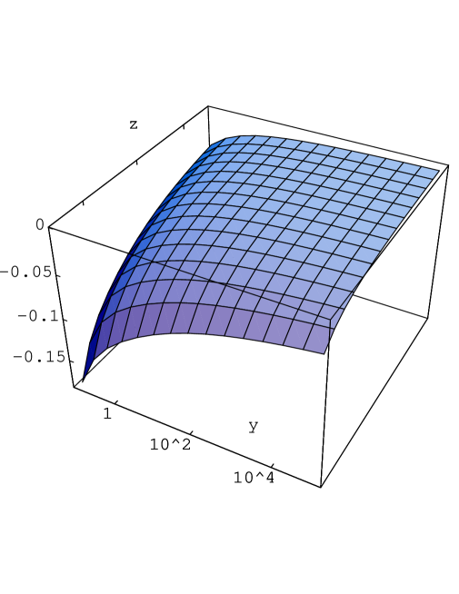
FIG. 2.: Graph of $M_{1}(1,y,z)$

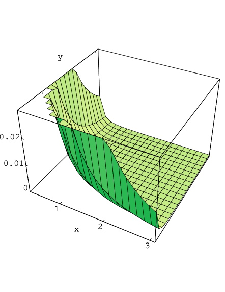
FIG. 3.: Graph of the second main minor $M_{2}(x,y,1)$

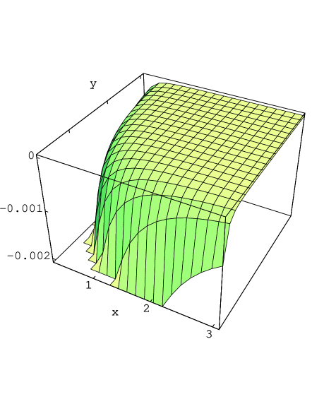
FIG. 4.: Graph of $M_{3}(x,y,1)$

REFERENCES

- [1] S. Kobayashi, K. Nomizu. Foundations of Differential Geometry, Vol. I, Interscience Publishers, New York London, 1963.
- [2] W. F. Donoghue, Monotone Matrix Functions and Analytic Continuation, Springer-Verlag, New York, 1974.
- [3] F. Kubo, T. Ando, Means of positive linear operators, Math. Ann. 246 (1980) 205–224.
- [4] P. M. Alberti, A. Uhlmann. Stochasticity and Partial Order, Deutscher Verlag der Wissenschaften, Berlin, 1981.
- [5] S. Amari. Differential Geometric Methods in Statistics, Lecture Notes in Statistics 28, Springer-Verlag, New York, 1985.
- [6] A. Uhlmann, Parallel transport and ”quantum holonomy”, Rep. Math. Phys. 24 (1986) 229–240.
- [7] A. L. Besse. Einstein Manifolds, Springer-Verlag, Berlin, Heidelberg, 1987.
- [8] T. Friedrich, Die Fisher-Information und symplektische Strukturen, Math. Nachr. 153 (1991) 273-296.
- [9] E. A. Morozova, N. N. Chentsov, Markov invariant geometry on state manifolds (in Russian), Itogi Nauki i Techniki 36 (1990) 69–102.
- [10] A. Uhlmann, A gauge field governing parallel transport along mixed states, Lett. Math. Phys. 21 (1991) 229–236.
- [11] J. Dittmann, G. Rudolph, A class of connections governing parallel transport along density matrices, J. Math. Phys. 33 (1992) 4148–4154.
- [12] A. Uhlmann, The metric of Bures and the geometric phase, in Groups and Related Topics (R. Gielerak et al., Eds. ), Kluwer 1992.
- [13] J. Dittmann, On the Riemannian geometry of finite dimensional mixed states, Sem. S. Lie 3 (1993) 73–87.
- [14] S. L. Braunstein, C. M. Caves, Statistical distance and the geometry of quantum states, Phys. Rev. Lett. 72 (1994) 3439–3443.
- [15] D. Petz, Geometry of canonical correlation on the state space of a quantum system, J. Math. Phys. 35 (1994) 780–795.
- [16] S. L. Braunstein, C. M. Caves, G. J. Milburn, Generalized uncertainty relations: Theory, examples, and Lorentz invariance, Annals of Physics 247 (1996) 135–173, quant-ph/9507004
- [17] D. Petz, Monotone metrics on matrix spaces, Linear Algebra Appl. 244 (1996 ) 81–96.
- [18] F. Hiai, D. Petz, G. Toth, Curvature in the geometry of canonical correlation, Stud. Sci. Math. Hung. 32 (1996) 235–249.
- [19] J. Twamley, Bures and statistical distance for squeezed thermal states, J. Phys. A: Math. Gen. 29 (1996), 3723–3731, quant-ph/9603019
- [20] Gh.-S. Paraoanu, H. Scutaru, Bures distance between two displaced thermal states, quant-ph/9703051
- [21] J. Dittmann, Yang-Mills equation and Bures metric, Lett. Math. Phys. 46 (1998) 281–287,quant-ph/9806018
- [22] J. Dittmann, A. Uhlmann, Connections and metrics respecting standard purification, to appear in J. Math. Phys. 1999, quant-ph/9806028
- [23] J. Dittmann, The scalar curvature of the Bures metric on the space of density matrices, to appear in J. Geom. Phys. 1999, quant-ph/9810012
- [24] A. Lesniewski, M. B. Ruskai, Monotone Riemannian metrics and relative entropy on non-commutative probability spaces, math-ph/9808016