icp - 990527

Quantum measurement breaks Lorentz symmetry

by

Ian C Percival

Department of Physics

Queen Mary and Westfield College, University of London

Tel: 0044 171 775 3289         Fax: 0044 181 981 9465 email: i.c.percival@qmw.ac.uk

Abstract

Traditionally causes come before effects, but according to modern physics things aren’t that simple. Special relativity shows that ‘before’ and ‘after’ are relative, and quantum measurement is even more subtle. Since the nonlocality of Bell’s theorem, it has been known that quantum measurement has an uneasy relation with special relativity, described by Shimony as ‘peaceful coexistence’. Hardy’s theorem says that quantum measurement requires a preferred Lorentz frame. The original proofs of the theorem depended on there being no backward causality, even at the quantum level. In quant-ph/9803044 this condition was removed. It was only required that systems with classical inputs and outputs had no causal loops. Here the conditions are weakened further: there should be no forbidden causal loops as defined in the text. The theory depends on a transfer function analysis, which is introduced in detail before application to specific systems.

PACS 03.65.Bz keywords: quantum, Bell, collapse, measurement, Lorentz, transfer, causality

99 May 27, QMW TH 99-07 To be submitted

1 Introduction p3

2 Deterministic systems p4
 2.1 Physical systems with inputs and outputs
 2.2 Transition and transfer pictures
 2.3 Combining systems
 2.4 Causal loops

3 Stochastic systems p15
 3.1 Transition and transfer pictures
 3.2 Background variables
 3.3 Independence
 3.4 Linked systems and causal loops

4 Space and time p23
 4.1 Time-ordering and causality
 4.2 Systems and ports in space and time
 4.3 Signalling transfer functions

5 Inequalities of the Bell type p25
 5.1 Quantum experiments in spacetime
 5.2 Background variables
 5.3 Bell-type experiments
 5.4 Bell inequalities
 5.5 Simplified and moving Bell experiments

6 Hardy’s theorem and the double Bell experiment p31
 6.1 Hardy’s theorem
 6.2 The double Bell experiment
 6.3 Breaking Lorentz symmetry

1 Introduction

Bell’s inequalities are a consequence of classical constraints on causal relations in spacetime, where here classical means non-quantum, as against nonrelativistic. Constraints such as the Bell inequality have significance for purely classical stochastic systems, as well as for quantum measurement theory. Here they are put in the context of a general theory of such constraints. This general theory follows from an application of a spacetime approach to the input-output theory of the engineers. The approach requires only that space and time should be put on a common basis, and that the spacetime constraints on causality should be clearly stated in the context of input-output systems. The rest, including Bell’s theorem, and the breakdown of Lorentz symmetry, follows.

Bell’s ideas on quantum measurement and related problems are put in a wider context within a general formalism. In this more general context, a double Bell thought experiment described here and in [14, 13] is used to demonstrate Hardy’s theorem that quantum measurements require a preferred Lorentz frame. The tension between Bell nonlocality and special relativity is well-known and has been discussed widely, for example by Shimony [16] Helliwell and Konkowski [11] and at length in the book by Maudlin [12].

In the famous controversy between Einstein and Bohr on quantum theory, Einstein found it difficult or impossible to accept nonlocal interactions. Bell’s theorem shows that nonlocality is unavoidable. Hardy’s theorem goes further by showing that quantum measurement requires a preferred Lorentz frame. It does not satisfy the conditions of Lorentz invariance. The original proofs of the theorem depended on there being no backward causality, even at the quantum level. The double Bell experiment does not. It combines two Bell experiments in a configuration resembling Einstein’s original special relativistic thought experiment with light signals. When combined with Lorentz invariance and Bell’s theorem, this leads to a forbidden causal loop with probability greater than zero. This is ruled out by a stochastic causal loop constraint, leading either to Hardy’s result or to other consequences that are very difficult to accept.

Causal loops are introduced first for deterministic systems and then for stochastic systems. There is a causal loop constraint for each. The transfer function theories of the Bell experiment and the double Bell experiment are presented.

2 Deterministic systems

2.1 Physical systems with inputs and outputs

Physical systems may be isolated or they may interact with one another. This work develops the theory of those systems whose interaction with other systems is restricted to discrete classical inputs and outputs with well-defined properties. System here refers to such a system.

Such systems are the elements of digital circuits as used in communications and computer technology. Many of the ideas presented here are taken from these fields, but there is an important difference. In technology it is conventional and convenient to treat space and time very differently. In physics, particularly relativistic physics, it is better to treat them far as possible on the same basis. In engineering, a system is restricted to a localized region of space, but is not usually considered to be restricted with respect to time. An engineering system which is restricted with respect to both space and time, for example a communication system with a signal confined to given intervals of time at the input and output, is an example of the kind of physical system treated here. Our physical systems are restricted to regions of spacetime in the same way that engineering systems are restricted in space. Of course, in practice, no engineering system lasts for ever, so all of them are like our systems, but this finite lifetime is often ignored in the engineering context.

The spacetime properties of our physical systems are so important that they are treated separately from the other properties, in order that the role of the spacetime properties can be seen as clearly as possible. So we start by treating systems and their interactions without considering where they are in spacetime, and introduce the spacetime relations and their properties afterwards.

A system may be entirely classical, or partly classical and partly quantum, but here the inputs and outputs are always classical, even though the rest of the system may be quantal. We treat quantum measurements and also other types of interaction between quantum systems and classical systems. We do not consider purely quantum systems except as a link between classical inputs and classical outputs. It is often helpful to treat these classical and classical-quantum systems as black boxes, whose only important property is the relation between the classical input and the classical output.

Every system $S$ contains classical input and output ports, which contain the inputs and outputs. We start by describing the properties of systems with only one input and one output port, whose inputs and outputs are discrete, with a finite number of possible states. The inputs are labelled $i$, with ${\cal N}(i)$ possible values, and the outputs are labelled $j$, with ${\cal N}(j)$ possible values.

Because the inputs and outputs are classical and discrete, their values can be measured, that is, they can be monitored, without affecting the evolution of the system. For continuous variables this is not true. Monitoring continuous variables always produces a perturbation. In classical theory the perturbation can be made arbitrarily small, but there are practical limits and also a quantum limit beyond which it is not possible to go. Quantum systems cannot be monitored without producing major changes in the system, except for special cases. These are the reasons for restricting our attention to systems with discrete classical inputs and outputs.

The simplest nondegenerate ports are binary ports with only two possible values. These are usually taken to be 0 and 1, although in some contexts we use $+$ and $-$ or even 1 and 2. Systems with only binary ports are binary systems, and these are the elements from which digital computers are built. Much of the theory will be illustrated using systems with binary ports.

The distinction between input and output ports is made by the different roles they play in the interaction of a system with its environment. Since each system is confined in spacetime, the environment is the spacetime environment. ‘Another system’ in the spacetime context may occupy the same region of space at a different time, so from the engineer’s viewpoint it is the same system.

As usual, input and output ports are distinguished by their causal relations with the system and its environment, which often includes other such systems. An input $i$ at the input port of a system $S$ is determined by its environment outside $S$. It affects the evolution of $S$ in general, and the outputs $j$ at the output ports in particular. The outputs affect the spacetime environment, but do not affect the rest of the system. The system is the physical link by which the input affects the output, which is its most significant role here. This is particularly important when the link between the inputs and outputs is a quantum system, as in a controlled quantum measurement.

We are concerned with the evolution of the system as it affects the causal relations between the inputs and outputs, which may be deterministic or stochastic.

2.2 Transition and transfer pictures

If $i$ determines $j$ uniquely, then the system is deterministic. Sections 2.2-2.4 deal with deterministic systems. Many important spacetime relations between inputs and outputs, for example ‘an input can have no influence on an earlier output’ are not treated in detail here. They have separate sections 4.1-4.3 to themselves.

A system may have many input and output ports which are separated from one another. We then use $i_{p}$ to represent the input at port $p$ and $j_{q}$ the output at port $q$. The value of all the inputs together is represented by $i=(i_{1},i_{2},\dots)$ and $j=(j_{1},j_{2},\dots)$ represents the value of all the outputs. We refer to $i$ and $j$ as the the input and the output. Both may be distributed among many ports, but this does not affect our definitions of the causal relations between the overall input $i$ and the overall output $j$, which are the same as for elementary systems with only one port of each kind, such as the one illustrated in figure 2.1a.

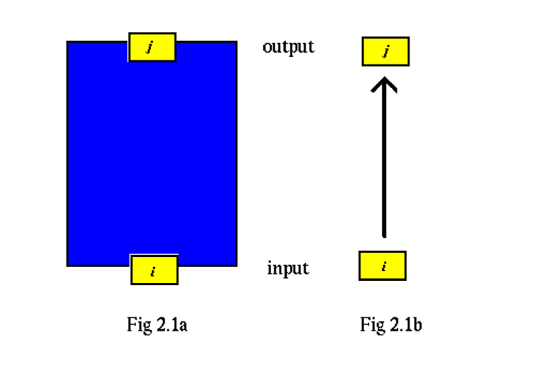
Figure 1: An elementary system with two ports.

Figure 2.1b is an alternative illustration of the system, where the arrow represents a causal link. This means that $j$ depends on $i$. If $j$ is independent of $i$, then the arrow is absent, and the same applies to the inputs and outputs at particular ports $i_{p}$ and $j_{q}$.

The number of possible values of $i$ and of $j$ are ${\cal N}(i)$ and ${\cal N}(j)$. For every value of the input $i$ there is a corresponding value of the output $j$, and the relation between them is the transition $i\rightarrow j$. The transitions for all inputs $i$ together can expressed as a function, the transfer function

$$F\hskip 28.45274pt\hbox{such that}\hskip 28.45274ptj=F(i).$$

We shall often treat the system as a black box, in which case the dependence of the outputs on the inputs, given by the transfer function, defines all the properties of a deterministic system that concern us. Either the transitions $i\rightarrow j$ for every $i$, or the single transfer function $F$ give the black box properties of the system.

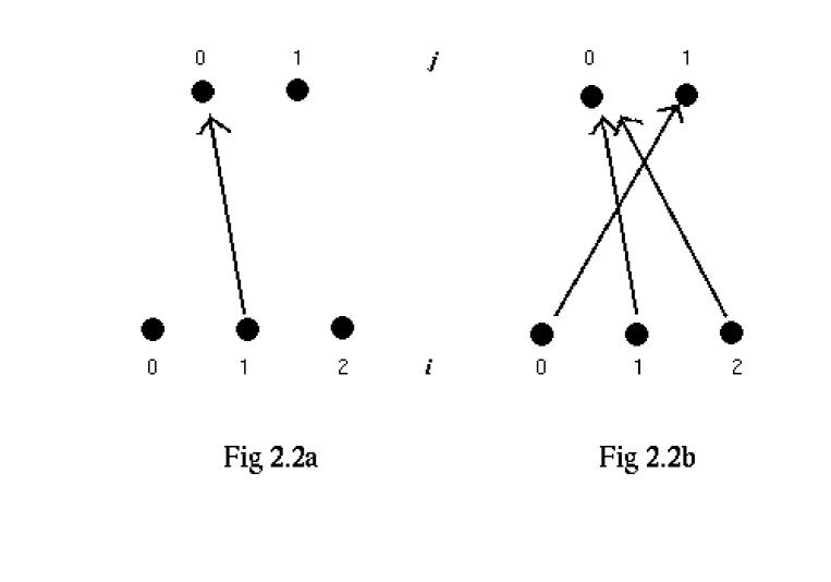
Figure 2: (a) A thin arrow represents a single transition, in this case from $i=2$ to $j=1$. (b) All transitions for a deterministic system, from each $i$ to some $j$. All these transitions together are represented by a transfer function $F$.

Figures 2.2a,b illustrate the properties of a system $S$ in more detail, by looking at the transitions between individual values of the input $i$ and the output $j$. A single transition from an $i$ to a $j$ can be represented by an arrow from $i$ to $j$, as in 2.2a for the transition $2\rightarrow 1$ in a system with three input values and two output values. For a given deterministic system, there is one transition for each value of $i$, and all together are given by the transfer function $F$, which can be represented by the transition arrows from all the input values $i$, as illustrated in figure 2.2b. The number of possible transitions ${\cal N}(i\rightarrow j)$ between the $i$ and the $j$ is given by the number of possible arrows pointing from an input value $i$ to an output value $j$.

Figure 2.3 illustrates all the possible transfer functions for an elementary binary system. $F_{0}$ and $F_{1}$ are degenerate, which means that the input has no effect on the output. When an output is degenerate, no signal is sent from the input and there is no causal connection between them.

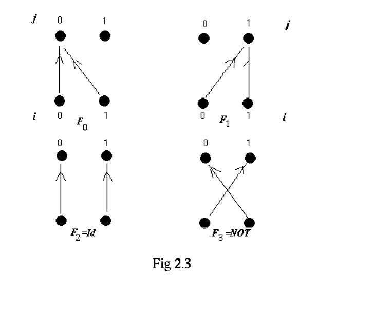
Figure 3: Transfer functions for an elementary binary system.

On the other hand, $F_{2}$ and $F_{3}$ are nondegenerate signalling transfer functions, recognizable as the familiar identity gate $Id$ and the $NOT$ gate.

For the system illustrated in figure 2.2, ${\cal N}(i)=3$, ${\cal N}(j)=2$. The number of possible arrows from an input value to an output value is just the product of the number of input values and the number of output values, giving

$${\cal N}(i\rightarrow j)={\cal N}(i){\cal N}(j).$$

Figure 4: The $3\times 2$ transitions $i\rightarrow j$ for system 2.2

Figure 5: The $2^{3}$ transfer functions $F$ for system 2.2

This is illustrated for our system in figure 2.4a. To define the dynamics of the system, we need the transfer function $F$, which corresponds to a set of arrows, one from every $i$ to some $j$. How many different possible transfer functions are there? This is illustrated for our example in figure 2.4b. For one $i$ there is a choice of ${\cal N}(j)$ possible arrows $i\rightarrow j$, for two $i$’s there is a choice of ${\cal N}(j)^{2}$ possible pairs of arrows, and for all ${\cal N}(i)$ allowed values of the input, there are ${\cal N}(j)^{{\cal N}(i)}$ possible choices for the ${\cal N}(i)$ arrows, so the number of possible transfer functions is

$${\cal N}(F)={\cal N}(j)^{{\cal N}(i)}.$$

The transition picture of the dynamics is based on the transitions, and the transfer picture is based on the transfer functions. The distinction between these pictures seems artificial at this stage, since they are trivially equivalent, but for the stochastic systems treated later it is crucial.

The number of possible transfer functions is usually much larger than the number of transitions. This is important for the theory of stochastic systems. We will often have to consider the space of transfer functions. This space is discrete for our systems, but often large in the sense that it consists of a large number of distinct points, each corresponding to one possible transfer function.

Binary systems, for which each of the inputs $i_{p}$ and outputs $j_{q}$ has only two possible values, are particularly simple and important. The gates which form the elements of digital circuits computers are examples, including the NOT, AND and control-NOT gates, together with the elementary binary system for which the transfer function is the identity.

A general deterministic system $S$ with two input and two output ports has a transfer function $F$ for which

$$(j_{1},j_{2})=F(i_{1},i_{2}).$$

Each output $j_{q}$ is a function $F_{j_{q}}(i_{1},i_{2})$ of the inputs, so $F$ can be expressed as a ‘vector’

$$F=(F_{1},F_{2}),\hskip 28.45274pt\hbox{where}\hskip 28.45274ptj_{1}=F_{1}(i_{1},i_{2}),\hskip 28.45274ptj_{2}=F_{2}(i_{1},i_{2}).$$

The causal links between the ports are illustrated in Figure 2.5a.

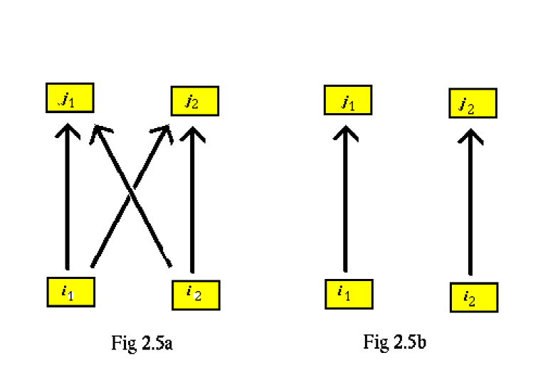
Figure 6: Causal links, (a) for a general system with two input and two output ports and (b) for the specific case when it is formed of two independent elementary subsystems

Suppose all four ports of the two subsystems are binary, then the total number of inputs or outputs is 4. There are $4\times 4=16$ possible transitions, and the total number of transfer functions is $4^{4}=256$.

2.3 Combining systems

Systems $S^{k}$ can be combined together in various ways to make a new system $S$, so that the $S^{k}$ become subsystems of $S$. We make the standard assumption that the causal relation between an input and an output of a subsystem $S^{k}$ is unaffected by this process. The external relations of a subsystem do not affect its internal dynamics. The transitions and the transfer functions are therefore unaffected.

Properties of different systems, such as transfer functions, are usually distinguished by an index, to distinguish them from properties of the same system, distinguished by a suffix. When we combine systems, the notation can become ambiguous, and either may be used.

Suppose there are two elementary systems $S^{1}$ and $S^{2}$, each with a single input and a single output port, with inputs and outputs $i^{1},i^{2}$ and $j^{1},j^{2}$ and transfer functions $F^{1}$ and $F^{2}$. If these subsystems are independent, then they can be considered together as a single system $S$, which is not elementary because it has two inputs $i_{1},i_{2}$ and two outputs $j_{1},j_{2}$. These may however, be considered together to form the input $i=(i_{1},i_{2})$ and the output $j=(j_{1},j_{2})$ of the system $S$, as illustrated in figure 2.6.

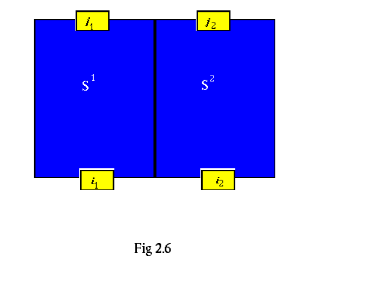
Figure 7: Combination of independent systems $S^{1}$ and $S^{2}$ to form a system $S$ with $i=(i_{1},i_{2})$, $j=(j_{1},j_{2})$

When a system $S$ is made from a combination of two separate and independent subsystems $S^{1},S^{2}$ in this way, the transfer functions $F_{j}=F^{j}$ have the special form

$$j_{1}=F^{1}(i_{1},i_{2})=F^{1}(i_{1}),\hskip 28.45274ptj_{2}=F^{2}(i_{1},i_{2})=F^{2}(i_{2}).$$

The port $j_{2}$ is not affected by $i_{1}$, and nor is $j_{1}$ affected by $i_{2}$. There are no signals between the subsystems, as illustrated in figure 2.5b. The total number of transitions and transfer functions is

$$N(i\rightarrow j)=N(i_{1}\rightarrow j_{1})+N(i_{2}\rightarrow j_{2})\hskip 28.45274pt\hbox{and}\hskip 28.45274ptN(F)=N(F^{1})N(F^{2}).$$

When all four ports are binary, then there are $2\times 2+2\times 2=8$ transitions and $2^{2}\times 2^{2}=16$ transfer functions. When compared with the general system with four binary ports described at the end of the previous section, the combined system has fewer transitions and far fewer transfer functions.

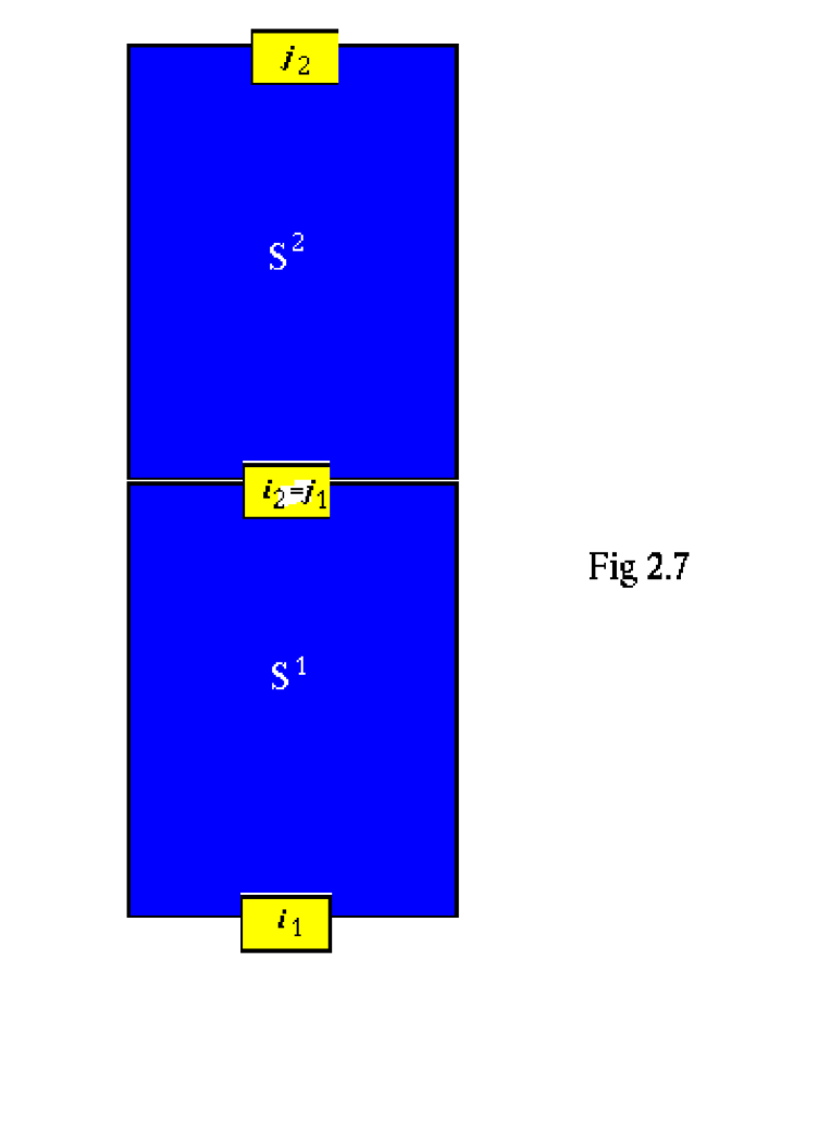
Figure 8: Systems $S^{1}$ and $S^{2}$ combined in series to form a system $S$.

Now suppose our two elementary systems are joined in series so that the output port of $S^{1}$ is the input port of $S^{2}$. As a black box, the combined system has only one input $i=i_{1}$ and one output $j=j_{2}$, which are illustrated in figure 2.7. Joining the systems has reduced the number of ports by one input and one output port, and

$$j=F^{2}(F^{1}(i))=F(i),\hskip 28.45274pt\hbox{where}\hskip 28.45274ptF=F^{2}\circ F^{1},$$

and the standard $\circ$ notation has been used for the composition of the transfer functions. The same function $F$ may result from different combinations of $F^{1}$ and $F^{2}$. The number of transfer functions is given by equation (2.3), with $i=i_{1},j=j_{2}$. Evidently there is a consistency condition for these two systems to be combined in series, that the output port $j_{1}$ must be of the same type as the input port $i_{2}$, and in particular that ${\cal N}(j_{1})={\cal N}(i_{2})$.

The generalization of the theory for two elementary systems to an arbitrary number of elementary systems is clear. For elementary systems in series, the same transition can result from many different paths through the input and output ports of the the subsystems, and the same transfer function from many different combinations of transfer functions for the subsystems.

The generalization to many systems is also clear for independent systems that are not elementary. But it is certainly not true for arbitrary combinations of systems which are joined by different input and outputs ports $i_{p}$ and $j_{q}$ as illustrated for some relatively simple cases in figures 2.8 and 2.9. Such arbitrary combinations include every digital communication system and every digital computer that has been built!

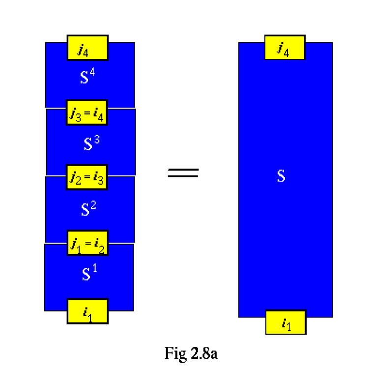
Figure 9: A chain of four subsystems connected in series.

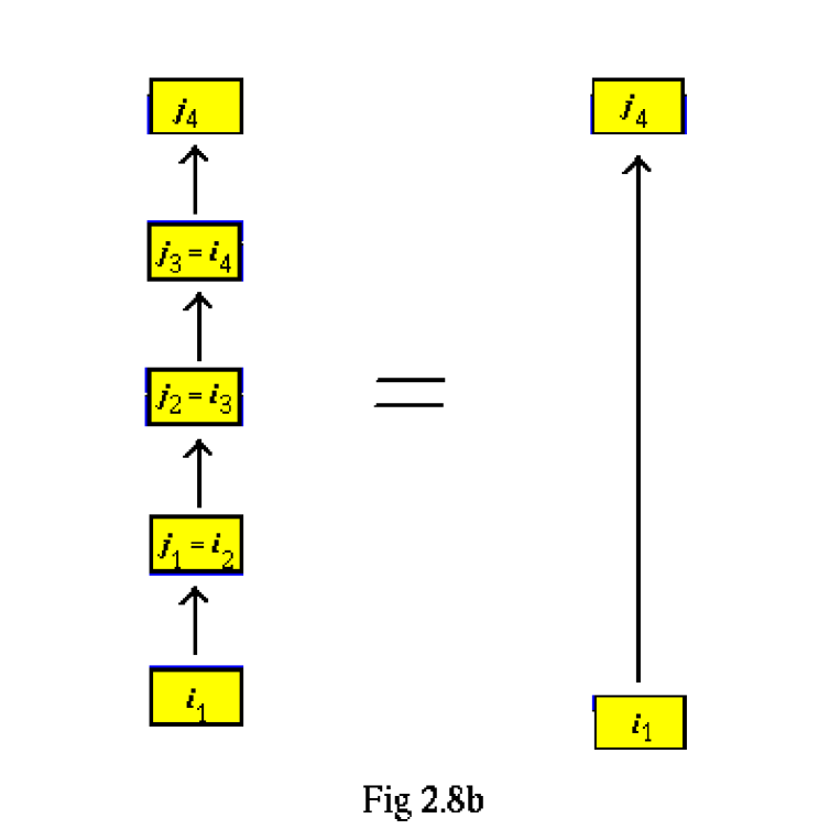
Figure 10: A chain of four subsystems connected in series: causal connections.

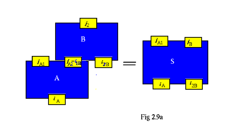
Figure 11: Systems joined by less than the maximum number of ports.

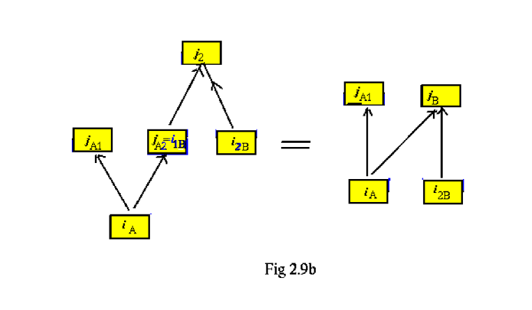
Figure 12: Systems joined by less than the maximum number of ports: causal connections.

We have seen that a system formed by the combination of the two independent systems has fewer possible transitions than for a general system with the same ports, and the the number of transfer functions for the combined system can be considerably less.

There are so many different kinds of linkages like this, that we will consider them independently as they arise.

2.4 Causal loops

Some of the following sections present the input and output in the context of space and time, which puts constraints on the possible ways of linking systems through their inputs and outputs, but in this section we ignore such constraints. Most of us believe it is not possible to form a causal loops because of their time relations, although some cosmologists who work with wormholes might disagree. Effects are expected to come after causes, outputs after inputs, so the final output from a chain of systems like that in figure 2.8 cannot be the same as the initial input. However, in relativity, time cannot be considered without space, and the spacetime relations of systems which include quantum measurements are particularly subtle.

We need to consider causal loops in the abstract first, to distinguish spacetime constraints from those that are independent of spacetime. We now demonstrate that there are such independent constraints.

We make the following provisional assumptions about deterministic systems:

AD1. A finite number ${\cal N}(S^{k})$ of subsystems $S^{k}$, with fixed input and output ports and transfer functions $F^{k}$ can be combined in any way to form a system $S$, provided that the corresponding input and output ports are consistent.

AD2. Combining systems does not change their transfer functions $F^{k}$.

For some collections of subsystems, these assumptions lead to a contradiction, as we now show.

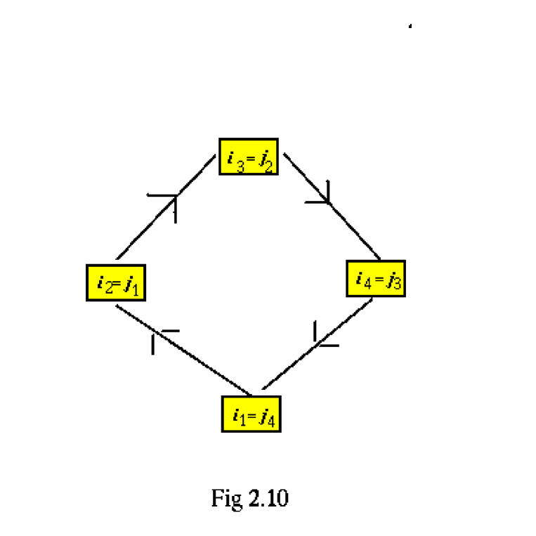
Figure 13: A causal loop formed from four subsystems.

Two or more subsystems may be linked together in a loop, which we shall call a causal loop, as illustrated in figure 2.10 for four systems.

Causal loops in spacetime are not the same as feedback loops in space. The output of a feedback loop is alway delayed with respect to the input, it comes to the same point in space, but later in time, whereas for a causal loop the output and input are the same, at one point in spacetime. A feedback loop may be unstable, whereas a causal loop can be forbidden.

In general, each system $S^{k}$ with $k=1,\dots{\cal N}(S)$ has input $i^{k}$ and output $j^{k}=i^{k+1}$, which is also the input to the next system. The corresponding transfer function is $F$, where $i^{k+1}=F^{k}(i^{k})$. The loop is closed by $j^{{\cal N}(S)}=i^{1}$, from which it follows that

$$i^{1}=F_{\rm loop}(i^{1}),\hskip 28.45274pt\hbox{where}\hskip 28.45274ptF_{\rm loop}=F^{{\cal N}(S)}\circ\dots\circ F^{2}\circ F^{1}.$$

Suppose, however, that in the case of the four subsystems illustrated in figure 2.10, all the ports are binary and the systems have transfer functions

$$F^{1}=F^{2}=F^{3}=Id,\hskip 28.45274ptF^{4}=NOT,$$

so the loop transfer function is $F_{\rm loop}=NOT$. Then from equation (2.9), $i^{1}=0$ implies $i^{1}=1$ and $i^{1}=1$ implies $i^{1}=0$, so there is a contradiction. This loop transfer function is forbidden. One of the assumptions must be wrong.

In general, a loop transfer function $F_{\rm loop}$ must have at least one input with an identical output if it is to be allowed. The inputs that satisfy this condition are the allowed inputs. If there is such an input, then the causal loop is allowed. If there is no such input, then the causal loop always leads to a contradiction. This combination is forbidden, so for any collection of subsystems which can be combined into a forbidden causal loop, one of the assumptions must be wrong.

This is the deterministic loop constraint.

This constraint does not depend on spacetime relations, but they are connected. For example, in classical nonrelativistic dynamics, effects always come after causes, so the assumption AD1 is always wrong: it is not possible to construct any causal loops, and the distinction between allowed and forbidden causal loops is irrelevant. So once the spacetime constraints are used, the loop constraint tells us nothing more. The same is true in classical special relativity.

This loop constraint has applications in classical general relativity, in which there are solutions of Einstein’s equations with ‘wormholes’. The problems of causality for these curved spacetimes with unusual topologies are sometimes discussed in terms of such violent acts as ‘shooting your grandmother before she conceives your father’. The deterministic loop constraint is a formal statement of this and also more gentle contradictions. However, these applications are not our main concern, for the deterministic loop constraint is used here as an introduction to the stochastic loop constraint of section 3.4, which can be applied quantum measurement.

3 Stochastic systems

3.1 Transition and transfer pictures

The theory so far has been restricted to deterministic systems. A system is deterministic if the value $j$ of the output is uniquely determined by the value of $i$ of the input. The dynamics of a deterministic system can be described in two ways that are trivially equivalent. The first is to give the output $j$ for each input $i$. This is the transition description. The other is to give the transfer function $F$ that defines this relation between outputs and inputs: $j=F(i)$. This is the transfer description.

More generally, classical systems are stochastic, or noisy. According to classical mechanics this is the result of interactions with other systems that cannot be eliminated. These other systems will be called the environment of the original system. For a system $S$, the distinction between another system $S^{\prime}$ of the type considered here and a part of the environment is a matter of convention, as it is in any other field in which there are systems and an environment. An example of a noisy system is a noisy NOT gate, in which, very occasionally, an input $i=0$ results in an output $j=0$ instead of the wanted $j=1$. In practice such noise cannot be avoided with certainty in digital circuits, although its probability can be made very low.

The results of quantum measurements are also typically stochastic, and according to ordinary quantum theory, this departure from determinism does not depend on the environment. Here we do not consider quantum systems on their own. A system always has inputs and outputs that are classical. In a quantum measurement, the inputs are the values of the macroscopic classical variables that determine which dynamical variables of the quantum system are being measured, and the outputs are the macroscopic classical states of the measuring and recording equipment that are produced by the measurement. So the system consists of the quantum system being measured, together with the essential classical parts of the apparatus being used to measure it.

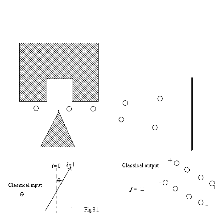
Figure 14: Stern-Gerlach experiment with variable direction of the magnetic field.

For a Stern-Gerlach experiment with individual atoms, the input is the orientation of the magnetic field, and the output is the classical record of the direction of spin with respect to the field, as illustrated in figure 3.1. We assume that the spin of the incoming atoms is vertically upwards. The orientation of the magnetic field determines which dynamical variable is being measured. According to Bohr, the result depends on the conditions under which the measurement is made [4, 5]. In some modern experiments, such as those to test nonlocality through Bell’s inequality, these conditions must be set or changed during the course of an experiment, and these are the inputs. Bohr did not mention this possibility.

For an experiment of the Bell type, the inputs are the orientations of the polarizers, and the outputs are the classical records of the measured polarization. In accordance with our insistence on discrete inputs, we consider only a finite number of possible orientations of the magnetic field for the Stern-Gerlach experiment or of the polarizers for the Bell experiment. The outputs are discrete because the spin components are quantized.

Just as for deterministic systems, the dynamics of stochastic systems can be described in terms of transitions $i\rightarrow j$ or in terms of transfer functions $F$, but for stochastic systems the relation between them is not trivial. In the transition picture the dynamics is defined by the probabilities of the transitions

$${\bf\rm Pr}\hskip 0.85358pt(i\rightarrow j)={\bf\rm Pr}\hskip 0.85358pt(j|i),$$

that is, the conditional probability of the output $j$ given the input $i$. Because there is always some output, these sum to unity for every $i$:

$$\sum_{j}{\bf\rm Pr}\hskip 0.85358pt(j|i)=1.$$

In the transfer picture, the dynamics is defined by probability that the system behaves like a deterministic system with transfer function $F$, for every possible $F$. These are the transfer function probabilities, or transfer probabilities, ${\bf\rm Pr}\hskip 0.85358pt(F)$, which sum to unity.

The conditional probability for finding the output $j$, when the input is $i$, is then given in terms of the transfer probabilities as

$${\bf\rm Pr}\hskip 0.85358pt(j|i)=\sum_{F}{\bf\rm Pr}\hskip 0.85358pt(F)\delta(j,F(i)).$$

This gives the transition probabilities in terms of the transfer probabilities. What about the other way round? There are nearly always many more transfer functions than transitions, the space of transfer probabilities is of higher dimension than the space of transition probabilities and so for a given set of transition probabilities ${\bf\rm Pr}\hskip 0.85358pt(j|i)$, there cannot in general be a unique set of transfer probabilities ${\bf\rm Pr}\hskip 0.85358pt(F)$. Deterministic systems, for which all probabilities are zero or one, are an important exception. Given the transition probabilities ${\bf\rm Pr}\hskip 0.85358pt(j|i)$, the transfer probabilities ${\bf\rm Pr}\hskip 0.85358pt(F)$ must satisfy equation (3.3), together with the inequalities and normalization of the transfer probabilities, which are

$$0\leq{\bf\rm Pr}\hskip 0.85358pt(F)\leq 1,\hskip 28.45274pt\sum_{F}{\bf\rm Pr}\hskip 0.85358pt(F)=1,$$

but (3.3) and (3.4) do not define the transfer probabilities uniquely.

We show later that the inequalities in (3.4) include the Bell inequalities.

Since there are usually more possible transfer functions than transitions, fixing the transition probabilities does not fix the transfer probabilities. For a system with given input and output ports, and without additional constraints, the number of independent transition probabilities is

$${\cal N}({\bf\rm Pr}\hskip 0.85358pt(i\rightarrow j))={\cal N}(i)({\cal N}(j)-1),$$

where the $-1$ comes from the condition that the transition probabilities from a given $i$ must sum to unity. The number of independent transfer probabilities ${\bf\rm Pr}\hskip 0.85358pt(F_{k})$ is ${\cal N}(F)-1$, which is usually greater. Within the space of sets of transfer probabilities, one for each $F_{k}$, there is a region of dimension given by equation (3.5) which is consistent with given transition probabilities. This we will call the consistent region of transfer probabilities, although strictly speaking it is a consistent region of sets of transfer probabilities, where a set contains a probability ${\bf\rm Pr}\hskip 0.85358pt(F_{k})$ for each transfer function $F_{k}$. This consistent region is the transfer picture equivalent of the set of transfer probabilities ${\bf\rm Pr}\hskip 0.85358pt(i\rightarrow j)$.

Frequently there are additional constraints, and they are often relatively simple to express in the transfer picture. The constraints may come from the physics, or they may be imposed in order to test a hypothesis, such as locality or relativistic invariance. In such cases the consistent region of transfer probabilities is reduced, sometimes to an empty region, in which case the constraints are incompatible, so that at least one of them must be wrong.

The causal relations for a noisy or stochastic system can be expressed in terms of signals just as they were for a deterministic system. If the probability ${\bf\rm Pr}\hskip 0.85358pt(F)$ of a signalling transfer function is always zero, then there are no corresponding signals for the noisy system. However, because the transfer probabilities are not unique, some care is needed in applying this principle.

Consider the elementary binary system of figure 2.3, with the degenerate transfer functions

$$F_{0}(i)=0,\hskip 28.45274ptF_{1}(i)=1$$

and the signalling transfer functions

$$F_{2}(i)=i,\hskip 28.45274pt\hbox{and}\hskip 28.45274ptF_{3}(0)=1,\hskip 2.84526pt\hskip 2.84526ptF_{3}(1)=0.$$

Suppose that the output $j$ is like the unbiassed toss of a coin, so that it is independent of the input, there is no signal or causal link from input to output, and

$${\bf\rm Pr}\hskip 0.85358pt(j=0)={\bf\rm Pr}\hskip 0.85358pt(j=1)={\scriptstyle{1\over 2}}.$$

The transition probabilities are then

$${\bf\rm Pr}\hskip 0.85358pt(0|0)={\bf\rm Pr}\hskip 0.85358pt(0|1)={\bf\rm Pr}\hskip 0.85358pt(1|0)={\bf\rm Pr}\hskip 0.85358pt(1|1)={\scriptstyle{1\over 2}},$$

which are unique.

But the transfer probabilities ${\bf\rm Pr}\hskip 0.85358pt(F)$ are not unique. One possibility is

$${\bf\rm Pr}\hskip 0.85358pt(F_{0})={\bf\rm Pr}\hskip 0.85358pt(F_{1})={\scriptstyle{1\over 2}},$$

in which the probability of the signalling transfer functions is zero. But another is

$${\bf\rm Pr}\hskip 0.85358pt(F_{2})={\bf\rm Pr}\hskip 0.85358pt(F_{3})={\scriptstyle{1\over 2}},$$

in which the probability of both signalling transfer functions is non-zero, even though there is no signal. The two sets of transfer probabilities (3.9) and (3.10) give the same set of transition probabilities (3.8). So for a stochastic system with a given set of transition probabilities, signalling transfer functions can have nonzero probability, despite there being no signal. A nonzero signalling transfer function probability does not necessarily indicate that there is a signal.

However, if there is a signal, then for every set of probabilities ${\bf\rm Pr}\hskip 0.85358pt(F)$ in the consistent region, at least one signalling transfer function has nonzero probability. Clearly this condition is not satisfied in the above example, but it is satisfied for every stochastic system with a signal.

3.2 Background variables

For the classical dynamics of an electrical circuit with resistors, those internal freedoms of the resistors which produce noise in the circuit are background variables, which are hidden, because we cannot see the motion of the ‘classical electrons’. Unlike some background variables of quantum mechanics, there is no physical principle that prevents the hidden variables of the classical circuit from becoming visible.

The same analysis can be applied to a quantum system prepared in a pure state, with a very important difference: the background variables are now hidden variables in principle and they need not have the properties of classical background variables. When they do not, the dependence of the output on the input cannot be classical: it must have a quantum component. The dependence of the outputs on the inputs cannot then be produced by any classical system. A quantum system can do things that a classical system cannot, which is the basis of technologies like quantum cryptography and quantum computation. If the system is in a black box, an experimenter can sometimes tell, just by controlling the input and looking at the output, that the output is linked to the input by a quantum system. This is why the study of hidden variables in quantum mechanics has had such important physical and practical consequences.

The variable $\lambda$ is a complete background variable of a system if the input $i$ and the background variable $\lambda$ together determine the output $j$. Another way of saying the same thing is that $\lambda$ determines the transfer function, which we then write as $F_{\lambda}$, so that

$$j=F_{\lambda}(i).$$

So the output $j$ depends only on the background variable $\lambda$ and the input $i$, and is uniquely determined by them. There are incomplete background variables for which the output is not uniquely determined, but we will suppose that they are supplemented if necessary by further background variables to make the output unique for a given $i$ and $\lambda$. From now on, all background variables are complete.

Given the probability ${\bf\rm Pr}\hskip 0.85358pt(\lambda)$ for the background variable, the probability of the output $j$, given the input $i$, is

$${\bf\rm Pr}\hskip 0.85358pt(j|i)=\int{\rm d}\lambda\hskip 2.84526pt{\bf\rm Pr}\hskip 0.85358pt(\lambda)\delta(j,F_{\lambda}(i)).$$

For a resistor, ${\bf\rm Pr}\hskip 0.85358pt(\lambda)$ is just the appropriate Boltzmann distribution.

Transfer function analysis is particularly suitable for background variables. For a particular system, two values of the background variable $\lambda$ which have the same transfer function $F_{\lambda}$ are completely equivalent. For a given input they result in the same output. Only the function $F_{\lambda}$ matters. So all the information that is needed about the probability distribution ${\bf\rm Pr}\hskip 0.85358pt(\lambda)$ is contained in the finite number of transfer probabilities for the transfer functions, which are

$${\bf\rm Pr}\hskip 0.85358pt(F)=\int{\rm d}\lambda\hskip 2.84526pt{\bf\rm Pr}\hskip 0.85358pt(\lambda)\delta(F,F_{\lambda}).$$

Once we have the transfer probabilities for a system $S$, we can forget about the probability distribution for the background variables of $S$. This is a great help, because the transfer probabilities usually live in a much simpler space.

We have seen that in general, systems with given transition probabilities do not have unique transfer probabilities. But we now see that systems with complete background variables do have unique transfer probabilities ${\bf\rm Pr}\hskip 0.85358pt(F)$, which therefore contain information about the relation of the system to its environment which is not contained in the transition probabilities. Also, for a given system, the transfer functions themselves can be treated as if they were discrete background variables.

The conditional probability for finding the output $j$, when the input is $i$, is then given by the sum

$${\bf\rm Pr}\hskip 0.85358pt(j|i)=\sum_{F}{\bf\rm Pr}\hskip 0.85358pt(F)\delta(j,F(i)),$$

which is usually much simpler in practice than the integral (3.12) over the background variable $\lambda$. This links the theory of background variables, including the possible hidden variables of quantum mechanics, with transfer functions.

But we should remember that the region of transfer probabilities which is consistent with the transition probabilities, is a general property of stochastic input-output systems, defined in terms of the transition probabilities, and independent of any hidden or background variables that there may or may not be.

3.3 Independence

Independence of systems is more subtle for stochastic systems than it is for deterministic systems. Subsystems of a classical stochastic system $S$ may be correlated by connecting inputs and outputs. But they may also be correlated through the environment, which is not part of $S$. Quantum systems produce their own very special kind of correlation, in which classical outputs corresponding to two separate and spatially separated measurements of the same quantum system can be correlated as a result of quantum entanglement. This is particularly important for Bell-type experiments.

These properties can be expressed in terms of background variables, or entirely in terms of the transfer functions, without the need for background variables. Now consider some special cases.

Two systems that are completely independent, without any correlation through their background variables, or through entanglement, have statistically independent transition probabilities. In preparation for application to Bell-type experiments, we introduce a different notation. If system $A$ has input $\alpha$ and output $a$, and system $B$ has input $\beta$ and output $b$, then the transition probabilities are statistically independent, that is

$${\bf\rm Pr}\hskip 0.85358pt(a,b|\alpha,\beta)={\bf\rm Pr}\hskip 0.85358pt(a|\alpha){\bf\rm Pr}\hskip 0.85358pt(b|\beta).$$

Each system has its transfer probabilities, ${\bf\rm Pr}\hskip 0.85358pt(F^{A})$ and ${\bf\rm Pr}\hskip 0.85358pt(F^{B})$. These are uncorrelated, so the corresponding transfer probability for the combined system $S$ has the form

$${\bf\rm Pr}\hskip 0.85358pt(F)={\bf\rm Pr}\hskip 0.85358pt(F^{A},F^{B})={\bf\rm Pr}\hskip 0.85358pt(F^{A}){\bf\rm Pr}\hskip 0.85358pt(F^{B}).$$

Using transfer functions we can distinguish between those correlations that come entirely through the effect of correlated background variables, and those that come through direct interaction between the systems. If there is no direct interaction, then there are no signals between $A$ and $B$ and we can find transfer functions $F^{A}$ which are functions of the input $\alpha$ alone and $F^{B}$ that are functions of $\beta$ alone, as before,

$$F^{A}(\alpha,\beta)=F^{A}(\alpha),\hskip 28.45274ptF^{B}(\alpha,\beta)=F^{B}(\beta),$$

such that the probabilities for all other transfer functions are zero.

However, if there is interaction through the background variables, then these separate transfer functions are correlated, so that

$${\bf\rm Pr}\hskip 0.85358pt(F^{A},F^{B})=\hskip-9.3894pt/\hskip 9.3894pt{\bf\rm Pr}\hskip 0.85358pt(F^{A}){\bf\rm Pr}\hskip 0.85358pt(F^{B})$$

In such a case there is correlation between the outputs, which is produced by the action of the background variables on the systems $A$ and $B$, but it is not possible to use this correlation to send signals between $A$ and $B$, because the probabilities of all signalling transfer functions are zero.

There is also another possibility, which occurs for experiments of the Bell type, for which there are signalling transfer functions between ports at $A$ and $B$, which always have non-zero total probability, yet it is not possible to use these to send signals, since it is not known which transfer functions operate. This is what happens when quantum systems violate the Bell inequality. Such signals are called weak signals. For a weak signal, the stochastic processes in the system can only be explained in terms of one or more non-zero signalling transfer probabilities, but it is not possible for us to control the input in such a way as to send a signal to the output corresponding to the signalling transfer function. The transfer functions are out of our control, as discussed using different terms by Shimony [16].

If the input and output of $A$ are both spatially separated from the input and output of $B$, then according to classical special relativity, there can be no signals from the input of $A$ (or $B$) to the output of $B$ (or $A$), but there can be correlation between the systems through interactions in their common past. When these systems are correlated, all the nonzero transfer probabilities satisfy (3.17) and (3.18). This is the locality condition, which can be applied to quantum systems also, whether they are supposed to have background (hidden) variables or not.

3.4 Linked systems and causal loops

Stochastic systems, like deterministic systems, can be combined by linking inputs and outputs. We do not go into the general theory of such combinations, only the parts that are important for quantum measurement theory.

There are constraints on the combinations that are independent of spacetime. Corresponding to the conditions AD1 and AD2 for deterministic systems, we have the stochastic system conditions

AS1. A finite number ${\cal N}(S^{k})$ of subsystems $S^{k}$, with fixed input and output ports and joint transfer probability given by ${\bf\rm Pr}\hskip 0.85358pt(F^{1},F^{2},\dots,F^{{\cal N}(S)})$, can be combined in any way to form a system $S$, provided that the corresponding input and output ports are consistent.

AS2. Combining systems does not change their joint transfer probability, given by ${\bf\rm Pr}\hskip 0.85358pt(F^{1},F^{2},\dots,F^{{\cal N}(S)})$.

The most significant difference between these assumptions and those for deterministic systems is that for the deterministic systems, we could assume that the conditions can be applied to the individual systems independently. For stochastic systems, we can no longer do this, because there can be correlations between transfer functions, due to the classical or quantum environment, or to quantum entanglement. So we have to use joint probabilities. For the particular case of probabilities that are either 0 or 1, the stochastic conditions become the same as the deterministic conditions, so there are systems for which the stochastic conditions cannot be satisfied, because they lead to forbidden causal loops.

We now show that a stochastic causal loop can lead to contradictions with finite probability under more general conditions.

Consider two elementary systems connected in series so that the output port of $S^{1}$ is the input port of $S^{2}$. The combined system has only one input $i=i_{1}$ and one output $j=j_{2}$, which are illustrated in figure 2.7. A transfer function $F$ for the combined system is obtained in terms of transfer functions $F^{1}$ and $F^{2}$ for the individual systems as in equation (2.8) for deterministic systems as

$$j=F^{2}(F^{1}(i))=F(i),\hskip 28.45274pt\hbox{where}\hskip 28.45274ptF=F^{2}\circ F^{1}.$$

If there is no correlation through background variables, or its quantum equivalent, then the probability ${\bf\rm Pr}\hskip 0.85358pt(F)$ of a given transfer function $F$ for the combined system is

$${\bf\rm Pr}\hskip 0.85358pt(F)=\sum_{F^{1},F^{2}}{\bf\rm Pr}\hskip 0.85358pt(F^{1},F^{2})\delta(F,F^{2}\circ F^{1}).$$

When there is no correlation between the transfer functions, through classical background variables or quantum entanglement, then we can put

$${\bf\rm Pr}\hskip 0.85358pt(F^{1},F^{2})={\bf\rm Pr}\hskip 0.85358pt(F^{1}){\bf\rm Pr}\hskip 0.85358pt(F^{2}),$$

a case of particular importance for the double Bell experiment that is to follow. In that case if, if ${\bf\rm Pr}\hskip 0.85358pt(F^{1})=\hskip-9.3894pt/\hskip 9.3894pt0$ for $S^{1}$ and ${\bf\rm Pr}\hskip 0.85358pt(F^{2})=\hskip-9.3894pt/\hskip 9.3894pt0$ for $S^{2}$, then ${\bf\rm Pr}\hskip 0.85358pt(F)=\hskip-9.3894pt/\hskip 9.3894pt0$ for the combined system $S$.

Just as in the case of deterministic systems, a chain of stochastic systems can be joined end to end to make a causal loop, with the transfer functions given by equation (2.9). For stochastic systems, causal loops are allowed if there are loop transfer probabilities, for which the probability of every forbidden loop transfer functions is zero. Otherwise there is a nonzero probability of a contradiction. So at least one of the assumptions must be wrong.

This is the stochastic loop constraint

An example of a forbidden stochastic causal loop can be constructed from the deterministic example of figure 2.10, with transfer functions given by equations (2.10). All we have to assume is that the probability ${\bf\rm Pr}\hskip 0.85358pt(F^{k})$ for the transfer function $F^{k}$ of system $S^{k}$ is not zero, and that the transfer functions are uncorrelated, so that

$${\bf\rm Pr}\hskip 0.85358pt(F^{1},F^{2},F^{3},F^{4})={\bf\rm Pr}\hskip 0.85358pt(F^{1}){\bf\rm Pr}\hskip 0.85358pt(F^{2}){\bf\rm Pr}\hskip 0.85358pt(F^{3}){\bf\rm Pr}\hskip 0.85358pt(F^{4})$$

There is then a nonzero probability for this forbidden deterministic loop transfer function, that is, a nonzero probability of a contradiction.

So the corresponding stochastic causal loop is itself forbidden.

As we shall see, the stochastic loop constraint has an application in quantum measurement. This is only possible because the nonlocality of quantum measurement imposes weaker spacetime constraints on causality than for classical deterministic or stochastic systems, or, indeed, for purely quantum systems.

Spacetime constraints are introduced in the next section.

4 Space and time

4.1 Time-ordering and causality

So far we have considered the causal relations between inputs, systems and outputs, without going into much detail on their spacetime relations. Does a particular input $i_{p}$ occur before or after another input, or an output, or, in special relativity, are they separated by a spacelike interval? These spacetime relations between the input and output ports are introduced quite separately from the causal relations. This is particularly important when applying the theory to the subtle spacetime causal relations of quantum measurement problems, like those of Bell experiments. We do not assume a priori that an output cannot be affected by an input that is separated from it by a spacelike interval. The relations between causality and spacetime must be introduced explicitly, and cannot be assumed.

In nonrelativistic Galilean dynamics, an input that takes place later than an output cannot affect it. This applies also in classical (non-quantum) special relativity, if ‘later’ than the output is interpreted to mean ‘entirely in or on the forward light cone of every spacetime point’ of the output. Each of these conditions forbids any kind of causal loop. Such relations between spacetime and causality are discussed in this chapter.

Classical nonrelativistic mechanics assumes that there is a universal time, represented by a variable $t$, defined everywhere in space. Given a system S, with any number of input and output ports, with input port $p_{\rm in}$ that comes after an output port $p_{\rm out}$, then there are no signals from $p_{\rm in}$ to $p_{\rm out}$. These nonrelativistic relations are independent of the location of the ports in space.

Classical relativistic dynamics is not so simple, since ‘before’ and ‘after’ then apply only to events with timelike or null separation. They are undefined for spacelike separations. Classically there are are no signals that go faster than the velocity of light, and so no signals between input and output ports that have spacelike separation. Relativistically, spatial relations become important.

Because the velocity of light is large, it is not always easy to control the spacetime relations experimentally. In particular, it is not easy to make the intervals between two ports of a laboratory experiment completely spacelike, because the time intervals are so short. This is one of the problems of experiments of the Bell type, leading to the ‘locality loophole’ which took a long time to close [1, 18, 17].

4.2 Systems and ports in space and time

We consider a finite number ${\cal N}(S)$ of systems $S$. Each system occupies a finite region of spacetime, which we will also denote by $S$, and a finite number of input ports and output ports. The ports of $S$ normally occupy regions of spacetime on the spacetime boundary of $S$. Systems can be connected through their input and output ports. Normally, they do not otherwise overlap in spacetime. It is sometimes convenient to show the spacetime relations of the ports in a spacetime diagram. Where the spacetime relations of special relativity are important, lines at 45^∘ represent the velocity of light. These are seen in the figure 5.1 and figures 5.2, 5.3 and 6.1 of the Bell and double Bell experiments.

4.3 Signalling transfer functions

These can be considered independently of spacetime, but their connection with the spacetime relations is so important that we treat them here.

Sometimes the input and output $\alpha,a$ in spacetime region $A$ are far from the input and output $\beta,b$ in spacetime region $B$, and causal connections for deterministic systems can the be expressed in terms of signals between the two regions, as follows:

$$F^{A}(\alpha\beta)=F^{A}(\alpha),\hskip 11.38109ptF^{B}(\alpha\beta)=F^{B}(\beta)\hskip 17.07164pt\hbox{(No signals between $A$ and B)}$$

$$F^{A}(\alpha\beta)=F^{A}(\alpha),\hskip 14.22636ptF^{B}(\alpha\beta)=\hskip-9.3894pt/\hskip 9.3894ptF^{B}(\beta)\hskip 28.45274pt\hbox{(Signal from $A$ to $B$ only)}$$

$$F^{A}(\alpha\beta)=\hskip-9.3894pt/\hskip 9.3894ptF^{A}(\alpha),\hskip 14.22636ptF^{B}(\alpha\beta)=F^{B}(\beta)\hskip 28.45274pt\hbox{(Signal from $B$ to $A$ only)}$$

$$F^{A}(\alpha\beta)=\hskip-9.3894pt/\hskip 9.3894ptF^{A}(\alpha),\hskip 14.22636ptF^{B}(\alpha\beta)=\hskip-9.3894pt/\hskip 9.3894ptF^{B}(\beta)\hskip 8.53581pt\hskip 28.45274pt\hbox{(Signals both ways),\hskip 8.53581pt}$$

where, for example, the inequality in (4.1b) means that $b$ depends explicitly on $\alpha$. Those transfer functions that allow signals are called signalling transfer functions. The signals are constrained by the conditions of special relativity, depending on whether the intervals between the inputs and outputs are spacelike or timelike. Where there are no signals, there are no corresponding signalling transfer functions, and no direct causal connection. However than can be a causal connection between the systems through classical background variables, or through interaction with the same quantum system.

A signalling transfer function for a signal from $A$ to $B$, where $A+B$ is a deterministic system, has the property that there must be at least two values of the input $\alpha$ of $A$, which we can call $0$ and $1$, and two values of the output $b$ of $B$, which we can call $+$ and $-$, such that when $\beta$ is constant, the input $0$ gives the output $+$ and the input $1$ gives the output $-$.

Now suppose the systems are stochastic. The signals and causal connections are then expressed in terms of the transition or transfer probabilities. In that case, for all consistent transfer probabilities, if there is a signalling transfer function for a signal from $A$ to $B$ with nonzero probability, with arbitrary ${\cal N}(a)$ and $N(b)$, the inputs can be restricted to a particular pair of values of $\alpha$ and a particular value of $\beta$, such that for all consistent transfer probabilities, the restricted transfer function also has nonzero probability. That is, the inputs can be restricted to a binary input for $\alpha$ and a single, degenerate, input value of $\beta$. This is important for the simplified Bell experiment discussed in section 5.5 and is used for the double Bell experiment of section 6.2.

5 Inequalities of the Bell type

5.1 Quantum experiments in spacetime

A quantum experiment consists of a quantum system linked to classical systems through preparation events $\alpha,\beta,\dots$, which are the inputs, and measurement events $a,b,\dots$, which are the outputs. The input $i=(\alpha,\beta,\dots)$ (in the singular) represents all the input events, and the output $j=(a,b,\dots)$ all the output events. Classical systems can similarly be prepared by input events and measured by output events.

Special relativity puts strong constraints on causality in spacetime. According to classical special relativity, causal influences such as signals operate at a velocity less than or equal to the velocity of light, so that an input event influences only output events in or on its forward light cone, and an output is only influenced by events in or on its backward light cone. They cannot operate over spacelike intervals, nor can they operate backwards in time. There is only forward causality.

Nevertheless, there can be correlations between systems with spacelike separation, due to background variables that originate in the region of spacetime common to their backward light cones. Causality which does act over spacelike intervals is generally called nonlocal causality, or simply nonlocality. It does not exist for relativistic classical systems. Correlation between events with spacelike separation is not sufficient evidence for nonlocality, since it can be due to common background variables.

Causality which acts backwards over timelike intervals means that the future influences the present, and the present influences the past. This is backward causality. This term will only be used when there is timelike separation between cause and effect. For our systems, with classical inputs and outputs, there can clearly be no backward causality, because it would be easy to connect a system with backward causality to an ordinary classical system with forward causality to produce a forbidden causal loop, using the method described in detail for the double Bell experiment of section 6.2. However, for purely quantum systems, we have no clear evidence either way as to whether or not there can be backward causality, and this presents a problem for Hardy’s original derivation of his theorem.

For our systems, these relations can be expressed in terms of classical inputs and outputs. Suppose that the input events or inputs $\alpha,\beta,\dots$ and output events or outputs $a,b,\dots$ are all so confined in spacetime that the interval between any pair of such events is well-defined as spacelike or timelike. The special case of null intervals is excluded, as it is not needed for our purposes. Since no signal can propagate faster than the velocity of light, an output $j_{\rm Y}$ depends only on those $i_{\rm X}$ that lie in its backward light cone, so that any variation of the other $i_{\rm X}$ makes no difference to $j_{\rm Y}$. This is illustrated in figure 5.1. This condition on the transfer function $F$ is a condition of forward causality, which applies to all those deterministic classical and quantum systems for which the input uniquely determines the output.

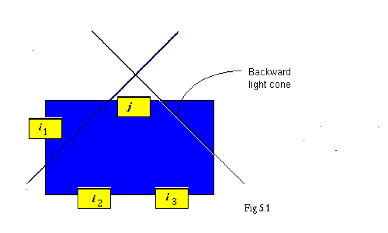
Figure 15: Classical system $S$ with spacetime relations of inputs and outputs. The output $j$ can depend on $i_{2}$ and $i_{3}$, but not on $i_{1}$

5.2 Background variables

The background variable $\lambda$ of noisy classical systems may be considered as an additional input, so it does not affect the causality relations between the inputs and outputs. Each of the transfer functions $F_{\lambda}$ satisfies the same causality conditions as the transfer function $F$ of a deterministic system. There is only forward causality.

The same applies to the transfer functions $F_{\lambda}$ of some quantum systems, but not to all. According to quantum mechanics, there are experiments for which the $F_{\lambda}$ with hidden variables $\lambda$ do not satisfy the conditions of forward causality: causality is nonlocal. These include experiments designed to test the violation of Bell’s inequalities. Experimental evidence has been overwhelmingly in favour of quantum mechanics, and also favours nonlocal causality through violation of inequalities. Nonlocal causality implies weak nonlocal signals in the sense of section 3.3.

The example of Bell experiments shows that the presence or absence of weak signals can tell us something about the properties of quantum systems. Because the background variables are hidden, weak signals cannot be used to send signals faster than the velocity of light. However, systems with weak signals have observable properties that cannot be simulated by any system whose inputs and outputs are linked by classical systems only.

5.3 Bell-type experiments

Einstein-Podolsky-Rosen-Bohm experiments, and Bell experiments which test Bell or Clauser-Holt-Horne-Shimony inequalities, are typical quantum nonlocality thought experiments. Real experiments have been based on the CHHS inequality, and use polarized photons. The analysis is similar for the Bell inequality and spin-half particles in magnetic fields, which we treat here. In one run of an experiment, two such particles with total spin zero are ejected in opposite directions from a central source. This stage of the preparation is not included in the input, as it happens for every run of the experiment, and the inputs $i$ are normally variable. Before the particles are detected, they pass into Stern-Gerlach magnetic fields. The classical settings of the orientations of the magnetic fields are the input events. The timing of these settings is crucial. The measurements, which include the classical recording of one of the two spin directions parallel or antiparallel to the field, are the output events.

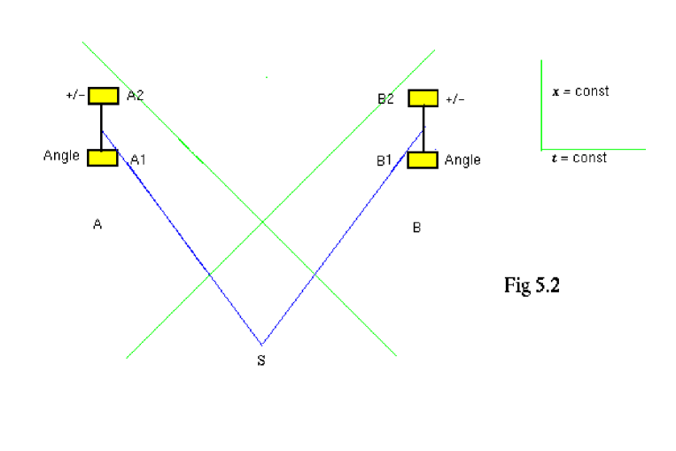
Figure 16: Spacetime diagram of Bell’s experiment. Thin diagonal lines at $45^{o}$ represent the velocity of light. At both $A1$ and $B1$, the angle is the setting of the angle of spin or polarization measurement, which is an input event, and at $A2$ and $B2$, $+/-$ represents the recording of the spin or polarization, an output event.

A spacetime illustration of a Bell experiment to test Bell’s inequality is given in figure 5.2. There are two inputs and two outputs, given by

$$i=(\alpha,\beta),\hskip 28.45274ptj=(a,b),$$

where one pair of inputs and outputs is confined to a spacetime region $A$ and the other is confined to a spacetime region $B$. The output $a$ is in the forward light cone of $\alpha$ and similarly for $b$ and $\beta$. The input preparation at $A$ must be separated by a spacelike interval from the output measurement at $B$ and vice versa, so both the input and output at $A$ are spatially separated from both the input and output at $B$. This is a considerable experimental challenge.

For local hidden variables, it is not possible to send even weak signals between $A$ and $B$, so there are only transfer functions of type (4.1a), and the other 3 types of transfer function have probability zero. It follows that the only transfer functions with nonzero probability have the form

$$F=(F_{A},F_{B}),\hskip 28.45274pt\hbox{where}\hskip 14.22636pta=F_{A}(\alpha),\hskip 14.22636ptb=F_{B}(\beta).$$

The conditional probability for the outcome $a,b$ given inputs $\alpha,\beta$ is then

$${\bf\rm Pr}\hskip 0.85358pt(a,b|\alpha,\beta)=\sum_{F_{A},F_{B}}{\bf\rm Pr}\hskip 0.85358pt(F_{A},F_{B})\delta(a,F_{A}(\alpha))\delta(b,F_{B}(\beta)).$$

This has the same form as Bell’s condition for locality, but in terms of transfer functions instead of hidden variables.

The spin of a particle is denoted $+$ when it is in the same direction as the field and $-$ when it is in the opposite direction. The output $j=(a,b)$ then consists of one of four pairs of spin components, $(++)$, $(+-)$, $(-+)$ and $(--)$, where the first sign represents the output at $A$ and the second sign the output at $B$. We will adopt a convention whereby the angles at $A$ and $B$ are measured from zeros that point in opposite directions, so that, for total spin zero, when the angles are equal, the measured signs of the spin components are the same, not opposite.

Consider first an experiment for which each of the magnetic field orientations at $A$ and at $B$ has only two possible angles, $\theta_{i}$ with $i=1,2$, the same pair of angles at $A$ and $B$ , with the above convention. Then the function $F_{A}$ can be labelled by a table of its output values $(\pm)$ for $i=1$ and $i=2$, and similarly for $F_{B}$. Thus if $a=+$ for $\alpha=1$ and $a=-$ for $\alpha=2$, we can denote $F_{A}$ by $F_{A}=[+-]$. The function $F$ can then be labelled by a table of 4 values, those for $A$ first, and those for $B$ second, eg $[+-,+-]$. For general functions $F$ we would have $2^{4}=16$ output values. But since we are assuming locality, $F$ has the form (5.3), and only 2 arguments each are needed to specify $F_{A}$ and $F_{B}$, so we need only 4 output values to specify $F$.

The number of independent probabilities ${\bf\rm Pr}\hskip 0.85358pt(F)={\bf\rm Pr}\hskip 0.85358pt(F_{A},F_{B})$ is then severely restricted by the fact that for opposite input orientations of the magnetic fields at $A$ and $B$, corresponding to $\theta_{A}=\theta_{B}$ and $\alpha=\beta$, the output signs $a,b$ must be the same. So when they are different the probability of $F$ is zero. Reversing the direction of all spins does not affect the probabilities. Thus all ${\bf\rm Pr}\hskip 0.85358pt(F)$ are zero except

$$P_{1}={\bf\rm Pr}\hskip 0.85358pt([++,++])={\bf\rm Pr}\hskip 0.85358pt([--,--]),$$

$$P_{2}={\bf\rm Pr}\hskip 0.85358pt([+-,+-])={\bf\rm Pr}\hskip 0.85358pt([-+,-+]),$$

where the right-hand equalities follow by symmetry. Notice that the two strings of signs, for $A$ and for $B$, are the same.

5.4 Bell inequalities

There are no contradictions with only two directions for the magnetic field. They can be handled with local hidden variables. But now consider 3 directions $\theta_{1},\theta_{2},\theta_{3}$, as in a Bell inequality. The values of $\alpha$ and $\beta$ are 1,2,3, and there are four independent probabilities, given by

$$P_{0}={\bf\rm Pr}\hskip 0.85358pt([+++,+++])={\bf\rm Pr}\hskip 0.85358pt([---,---]),$$

$$P_{1}={\bf\rm Pr}\hskip 0.85358pt([-++,-++])={\bf\rm Pr}\hskip 0.85358pt([+--,+--]),$$

$$P_{2}={\bf\rm Pr}\hskip 0.85358pt([+-+,+-+])={\bf\rm Pr}\hskip 0.85358pt([-+-,-+-]),$$

$$P_{3}={\bf\rm Pr}\hskip 0.85358pt([++-,++-])={\bf\rm Pr}\hskip 0.85358pt([--+,--+]).$$

From these transfer probabilities, we can obtain the known transition probabilities for experiments in which $\alpha,\beta$ with $i=1,2,3$ correspond to the three orientations $\theta_{i}$ of the fields. ${\bf\rm Pr}\hskip 0.85358pt(ab|\alpha\beta)$ is given by adding together the probabilities for which $a$ appears in position $\alpha$ in the first sequence of signs, and $b$ appears in position $\beta$ in the second sequence:

$${\bf\rm Pr}\hskip 0.85358pt(++|11)={\bf\rm Pr}\hskip 0.85358pt(--|11)=P_{0}+P_{1}+P_{2}+P_{3}=1/2\hskip 28.45274pt\hbox{and cyclic,}$$

$${\bf\rm Pr}\hskip 0.85358pt(++|23)={\bf\rm Pr}\hskip 0.85358pt(--|23)=P_{0}+P_{1}\hskip 28.45274pt\hbox{and cyclic,}$$

$${\bf\rm Pr}\hskip 0.85358pt(+-|23)={\bf\rm Pr}\hskip 0.85358pt(-+|23)=P_{2}+P_{3}\hskip 28.45274pt\hbox{and cyclic,}$$

where the cyclic permutations permute 1,2 and 3 but not 0.

The equations can be solved for the $P_{k}$, all of which must be nonnegative. Their solutions, with resultant conditions on ${\bf\rm Pr}\hskip 0.85358pt(++|\alpha\beta)$, ${\bf\rm Pr}\hskip 0.85358pt(+-|\alpha\beta)$ are

$$2P_{0}={\bf\rm Pr}\hskip 0.85358pt(++|23)+{\bf\rm Pr}\hskip 0.85358pt(++|31)+{\bf\rm Pr}\hskip 0.85358pt(++|12)-{1\over 2}\geq 0\hskip 28.45274pt\hbox{and cyclic,}$$

$$2P_{1}={1\over 2}+{\bf\rm Pr}\hskip 0.85358pt(++|23)-{\bf\rm Pr}\hskip 0.85358pt(++|31)-{\bf\rm Pr}\hskip 0.85358pt(++|12)\geq 0\hskip 28.45274pt\hbox{and cyclic,}$$

$$2P_{1}={\bf\rm Pr}\hskip 0.85358pt(+-|31)+{\bf\rm Pr}\hskip 0.85358pt(+-|12)-{\bf\rm Pr}\hskip 0.85358pt(+-|23)\geq 0\hskip 28.45274pt\hbox{and cyclic}.$$

The inequalities (5.7a,b) are always satisfied, but (5.7c) gives the Bell inequalities [2], chapter 2, his equation (15). Bell uses the same origin for the angles at $A$ and $B$, so his opposite signs are the same signs here, and his expectation values of products are

$$P({\bf b},{\bf c})=4{\bf\rm Pr}\hskip 0.85358pt(+-|23)-1\hskip 28.45274pt\hbox{and cyclic}.$$

The condition of weak nonlocality, the condition that the transfer function probabilities should all be non-negative, and the condition that sums over them are all less than or equal to 1, provide a systematic method for obtaining inequalities of the Bell type.

Inequalities of the Bell type follow from the condition that all transfer functions have positive or zero probabilities, which suggests the use of the methods of linear programming [14].

Since quantum mechanics violates the Bell inequalities, it is weakly nonlocal, and there is at least one weak signalling or nonlocal transfer functions $F^{\rm s}$ or $F_{\rm NL}$ with nonzero probability ${\bf\rm Pr}\hskip 0.85358pt(F^{\rm s})$. Using the notation of figure 5.2, there is a weak signal from $A1$ to $B2$ or from $B1$ to $A2$, or both.

It is here that special relativity comes in. The experiment is invariant for a rotation of $\pi$ that interchanges $A$ and $B$. This rotation is an element of the Lorentz group. So if there is a non-zero probability of a weak signal in one direction, it follows from invariance under this element of the group that there must also be a non-zero probability for a weak signal in the other. By Lorentz invariance there must be weak signals in both directions. The violation of the Bell inequality is not enough on its own to ensure this.

We will use this Lorentz invariance as an additional (spacetime) assumption for stochastic systems:

AS3 For flat spacetime, the laws of physics are invariant under all elements of the Lorentz group.

5.5 Simplified and moving Bell experiments

The proof of Bell’s theorem required at least three orientations of the polarizers, but its consequences can be expressed in terms of the transfer function of a simplified Bell experiment, using the results presented at the end of section 4.3. The spacetime configuration is the same as previous two experiments, illustrated in figure 5.2. But the input at $A$ has only one value $\theta_{1}$. The input at $B$ has two values:

$$\theta_{1}:\hskip 2.84526pti=1,\hskip 28.45274pt\theta_{2}:\hskip 2.84526pti=2.$$

There are four possible output values $j$ given by

$$(a+,b+)=\hskip 2.84526pt++,\hskip 8.53581pt(a+,b-)=\hskip 2.84526pt+-,\hskip 8.53581pt(a-,b+)=\hskip 2.84526pt-+,\hskip 8.53581pt(a-,b-)=\hskip 2.84526pt--,$$

where the first sign is for $i=1$ and the second for $i=2$, and where the second short form with just the two signs is used hereafter.

If $i=1$, corresponding to the same angle at $A$ and $B$, measured, as usual, from zeros that are an angle $\pi$ apart, then $j=++$ or $j=--$. Consider the $++$ case. There are four possible transfer functions. For the local degenerate transfer functions, the sign at $A$ is independent of the angle at $B$, so $F_{1}$ and $F_{4}$ are local. For nonlocal (NL) or signalling transfer functions, the sign at A depends on the angle at $B$, so $F_{2}$ and $F_{3}$ are nonlocal.

By Bell’s theorem and Lorentz invariance, both of the nonlocal transfer functions have non-zero probability:

$${\bf\rm Pr}\hskip 0.85358pt(F_{2})>0,\hskip 28.45274pt{\bf\rm Pr}\hskip 0.85358pt(F_{3})>0.$$

This simplified Bell experiment, like the full Bell experiment, is depicted in figure 5.2 at rest with respect to a laboratory frame. Now we make the whole experiment move uniformly, so that it is at rest in a frame that is moving with respect to the laboratory frame, as represented in figure 5.3. In this figure $x$ and $t$ are position and time coordinates in the moving frame.

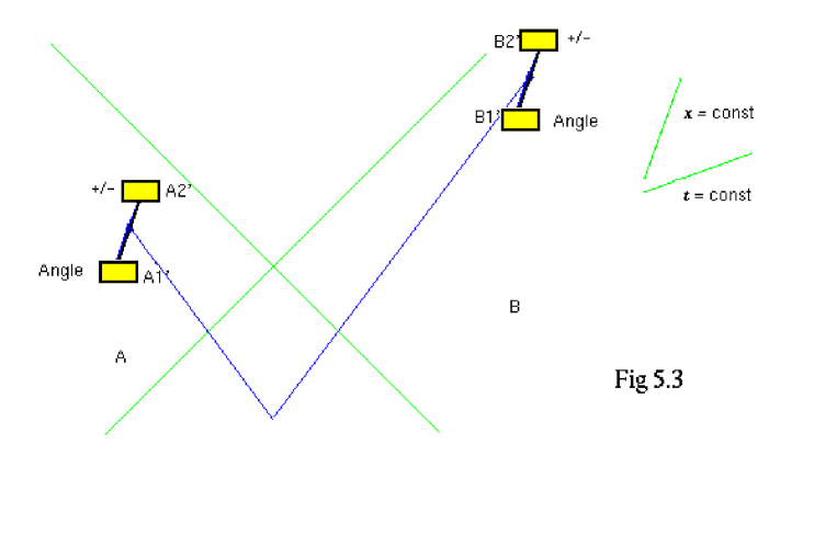
Figure 17: Spacetime picture of moving Bell experiment

The simplified moving Bell experiment is one component of the double Bell experiment which follows. Another component is a second simplified moving Bell experiment which moves with equal speed in the opposite direction, whose spacetime picture is a reflection of figure 5.3 in a vertical axis.

6 Hardy’s theorem and the double Bell experiment

6.1 Hardy’s theorem

Hardy’s theorem [9] goes further than Bell’s theorem on nonlocality of quantum measurement. It states that any dynamical theory of measurement, in which the results of the measurements agree with those of ordinary quantum theory, must have a preferred Lorentz frame. The theorem does not determine this frame.

Hardy originally presented the theorem through a thought experiment involving two matter interferometers, one for electrons and one for positrons, with an intersection between them that allows annihilation of the particles to produce gamma rays. The proof of the theorem depends on an assumption, which is that there is no backward causality in quantum systems. As discussed in section 5.1, we have no hard evidence for or against such backward causality. On the other hand, given a choice between backward causality in quantum systems and the breakdown of Lorentz invariance, it is not so clear which distasteful choice we should make. Without the assumption, this proof breaks down.

A different derivation based on classical links between two Bell experiments is given in [14, 13]. This is the double Bell experiment. The proof of Hardy’s theorem using the double Bell experiment is independent of any assumptions about causality in the quantum domain. It depends on causal relations between classical inputs and outputs, using the transfer picture, and the stochastic loop constraint of section 3. It is also assumed that the results of the separate Bell experiments are not correlated through some unsuspected background correlation. It would be remarkable if it were present, but a more complicated multiple Bell experiment shows that the theorem is independent even of this assumption. The multiple Bell experiment is described in [14], but not here.

6.2 The double Bell experiment

Einstein’s old simultaneity thought experiment used classical light signals from a source and two pairs of receivers, each pair in a different moving frame. We replace this by two simplified moving Bell experiments, each in a different frame and then show that the assumption of invariance under Lorentz transformations, together with further assumptions that are discussed in detail, leads to a forbidden causal loop with nonzero probability. So, given the further assumptions, there is no Lorentz invariance.

Here is the argument. It does not assume weak locality.

The double Bell experiment is a combination of two simplified moving Bell experiments, as defined at the end of the previous section, with two classical links, as illustrated in figure 6.1

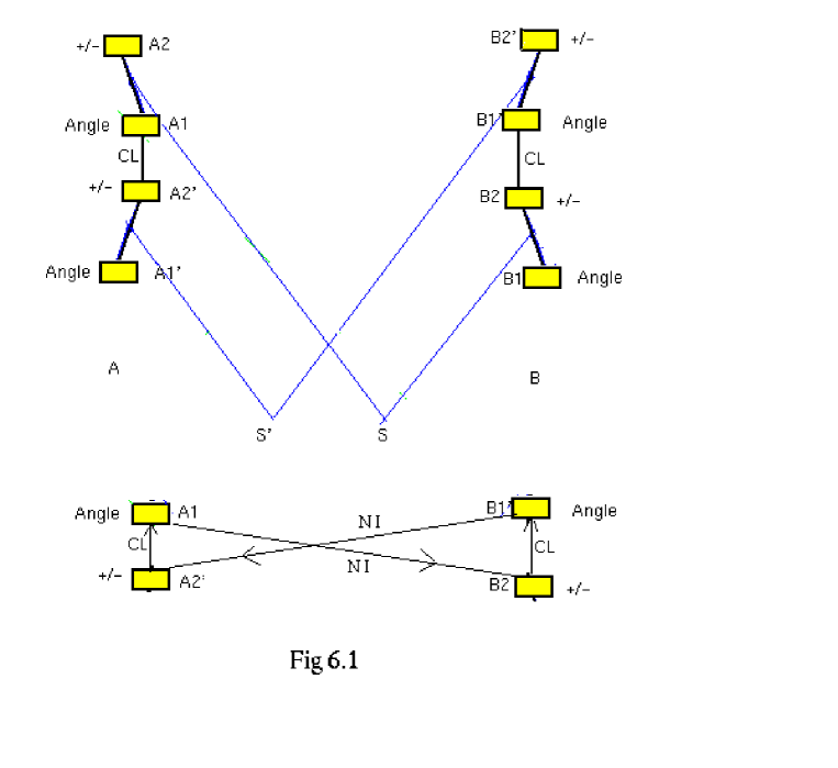
Figure 18: Spacetime diagram of the double Bell experiment. The meaning of the symbols corresponds to their meaning in the figures 5.2 and 5.3. The primed symbols belong to one Bell experiment, and the unprimed to the other. As usual $A$ and $B$ represent spatially separated parts of the full experiment, so there are four ports on each side. Notice that both the ports of each experiment at $A$ are spatially separated from both the ports of each experiment at $B$. CL are classical links, by which an output from each experiment determines the input to the other.

The two Bell experiments are independent at the quantum level, but they are linked classically so that the output $A2^{\prime}$ controls the input $A1$, which is in its future lightcone, and the output $B2$ controls the input $B1^{\prime}$. There are two significant nonlocal interactions NI. One is the setting of the angle at $A1$ affecting the measurement at $B2$, and the other is the setting of the angle at $B1^{\prime}$ affecting the measurement at $A2^{\prime}$. This is an unusual thought experiment, in that the variable input orientations of the magnetic fields at $A1$ and B1^′ are determined entirely by outputs. The causal loop structure is clearly seen in the laboratory.

The causal loop is

$${A2}^{\prime}\longrightarrow^{\hskip-14.22636pt\rm CL}\hskip 2.84526pt{A1}\longrightarrow^{\hskip-14.22636pt\rm NI}\hskip 2.84526pt{B2}\longrightarrow^{\hskip-14.22636pt\rm CL}\hskip 2.84526pt{B1}^{\prime}\longrightarrow^{\hskip-14.22636pt\rm NI}\hskip 2.84526pt{A2}^{\prime},$$

where NI represents the nonlocal interaction of one or other of the Bell experiments, and CL represents one of the classical links. Section 5.5 on the simplified moving Bell experiment, shows that both the nonlocal transfer functions must have nonzero probability. All inputs and outputs are binary, and with an appropriate convention for the labelling inputs and outputs, the nonlocal interactions are both equivalent to the identity gate $Id$. We are free to choose the classical links at will. We choose the link at $A$ to be the identity, and the link at $B$ to be the $NOT$ gate. The loop transfer function is then a $NOT$ gate, so it is a forbidden causal loop, and its probability is not zero.

This is forbidden by the stochastic loop constraint, so AS1, AS2 or the Lorentz assumption AS3 of section 3.4 must be false. Since there is nothing to prevent us from combining the two Bell experiments and the two classical links together in the configuration of a double Bell experiment, AS1 is satisfied, so the problem must be AS2 or Lorentz, and we had better look very carefully at AS2: combining systems does not change their joint transfer probability.

Two of the systems are deterministic gates, the other two are stochastic single Bell experiments. Before they are combined they have independent transfer probabilities, so according to AS2, this independence should be preserved when they are combined to make the double Bell experiment.

It is a fundamental assumption of modern experimental physics that we can control and monitor physical systems using deterministic digital gates, with well-defined ports, such that the only interaction between another system and a gate is through its ports. If this were not true we could not reliably use digital circuits for monitoring and controlling physical systems. So unless we are prepared to question the basis of almost all modern experimental physics, the problem cannot be AS2 as it applies to the interaction between the classical gates and the single Bell experiments, and between one gate and another.

The only remaining possibility is that AS2 should be wrong because the joint transfer probabilities of the two Bell experiments are changed as a result of combining them through the gates. This seems highly unlikely and appears to be ruled out by the multiple Bell experiment of [14].

Otherwise we have to conclude that AS3 is wrong, that in flat spacetime, the laws of physics are not invariant under the operations of the Lorentz group.

The double Bell experiment is described here as a thought experiment. It might be worth performing as a real experiment, but this is not clear. The results of the double Bell thought experiment follow from the results of an ordinary single Bell experiment, and some very general assumptions about independence of systems. These assumptions are at the foundation of almost all modern experimentation. The assumptions can be checked directly, and more simply, without performing the double Bell experiment itself.

However it becomes even more important than before to close the final detection loophole in the single Bell experiment, since it is assumed in our derivation that inequalities of the Bell type are violated with the right spacetime relations between the input and output ports, and this has not yet been fully confirmed experimentally, because of the loophole.

The double Bell experiment as presented here would be difficult to perform in the laboratory, because the apparatus of the two single Bell components would have to be move fast enough to produce a time dilation greater than the summed delays between the inputs and outputs of the Bell experiments and classical links. A more practical static double Bell experiment is presented in [14, 13], using optical fibre delay lines. Unfortunately, it was not realized when that paper is written, that the introduction of the time delays destroys the $\pi$-rotation symmetry of its component single Bell experiment, so it can’t be used to invalidate Lorentz invariance without additional assumptions.

It might be interesting to do the static experiment, even if it does produce the results expected from ordinary quantum theory, because it might have a weak causal loop, and no experiment to date has been set up with even the possibility of such a loop. Like the moving experiment the static experiment has no classical input in the usual sense, because the inputs of the individual simplified Bell experiments are controlled entirely by two of their outputs. Hence the loop.

6.3 Breaking Lorentz symmetry

We conclude that quantum measurement in general, and Bell nonlocality in particular, break Lorentz symmetry.

Claimed Lorentz-invariant realistic theories of quantum measurement [6, 3, 15, 8] and also [2], chapter 22, appear to conflict with Hardy’s theorem and our conclusions. It would be interesting to apply these theories to the double Bell experiment to find out how. For some of these theories the apparent conflict may lie in the different meanings given to ‘Lorentz invariant’ as it applies to quantum measurement theory.

Any localized system, any macroscopic system, any planet, breaks Lorentz symmetry, and causes other systems in its neighbourhood to obey a dynamics with a preferred frame. This is not unusual, it is the general rule for both classical and quantum localized systems. We can restore Lorentz symmetry for a system $S$ by enlarging $S$ to include the system that breaks the symmetry. Conversely, if we find a dynamical behaviour that breaks the symmetry, the first thing to do is look for a localized system in the environment that causes it. This could be provided by a field, as discussed for quantum measurement in [13].

But we need to break Lorentz symmetry in such a way that weak signals can propagate faster than the velocity of light, which is not true for the symmetry breaking due to ordinary localized systems. This situation is similar to the symmetry-breaking of quantum field theory in at least one respect: processes that are forbidden when the symmetry is respected become possible when it is broken. These issues, and the necessity of a consistent definition of simultaneity, are discussed in [13], but there is not yet an adequate theory of such Lorentz symmetry-breaking.

Acknowledgements I thank the Group of Applied Physics of the University of Geneva and the Institute of Physics and Astronomy of the University of Aarhus for their hospitality, also Gernot Alber, Lajos Diósi, George Ellis, Nicolas Gisin, Lucien Hardy, Klaus Molmer, Sandu Popescu and a large fraction of the Physics Department at QMW for stimulating discussions. I also thank the UK EPSRC and the Leverhulme Trust for financial support during the period of the research.

Notation

$S$ system, $i$ input value, $j$ output value, ${\cal N}(n)$ number of possible values of $n$, $p$,$q$ port labels, $i_{p},j_{q}$ input or output value at input or output port. $i\rightarrow j$ transition. $F$ transfer function. $k$ system or transfer function label. S^k $k$th system. $F^{k}$ transfer function for system S^k. $F_{k}$ one of several transfer functions for a single system, $F_{\rm loop}$ loop transfer function.

An alternative notation for systems is $A$, $B$, and corresponding inputs $\alpha$, $\beta$ and outputs $a$, $b$.

References

- [1] A. Aspect. Bell’s inequality test: more ideal than ever. Nature, 398:189–190, March 1999.
- [2] J. Bell. Speakable and Unspeakable in Quantum Mechanics. Cambridge University Press, Cambridge, England, 1987.
- [3] K. Berndl, D. Dürr, S. Goldstein and N. Zanghi. Nonlocality, Lorentz invariance and Bohmian quantum theory. Phys. Rev. A, 53:2062–2073, 1996.
- [4] N. Bohr. Can quantum-mechanical description of physical reality be considered complete? Phys. Rev., 48:696–702, 1935.
- [5] N. Bohr. Can quantum-mechanical description of physical reality be considered complete? In J. Wheeler and W. Zurek, editors, Quantum Theory and Measurement, pages 145–151, Princeton,N.J., 1983. Princeton Univ.
- [6] H.-P. Breuer and F. Petruccione. Relativistic formulation of QSD. J. Phys. A, 31:33, 1998.
- [7] R. Clifton and P. Niemann. Hardy’s theorem for two entangled spin-half particles. Phys. Lett. A, 166:177–184, 1992.
- [8] G.-C. Ghirardi, R. Grassi and P. Pearle. Relativistic dynamical reduction models: General framework and examples. Foundations of Physics, 20:1271–1316, 1990.
- [9] L. Hardy. Quantum mechanics, local realistic theories and Lorentz-invariant realistic theories. Phys. Rev. Lett., 68:2981–2984, 1992.
- [10] L. Hardy. Quantum optical experiment to test local realism. Phys. Lett. A, 167:17–23, 1992.
- [11] T. Helliwell and D. Konkowski. Causality paradoxes and nonparadoxes: classical superluminal signals and quantum measurements. Am. J. Phys., 51:996–1003, 1983.
- [12] T. Maudlin. Quantum Non-locality and Relativity. Blackwell, Oxford, 1994.
- [13] I. Percival. Cosmic quantum measurement . quant-ph, 9811089, 1998.
- [14] I. Percival. Quantum transfer functions, weak nonlocality and relativity. Phys. Lett. A, 244:495–501, 1998.
- [15] T. Samols. A stochastic model of a quantum field theory. J. Stat. Phys., 80:793–809, 1995.
- [16] A. Shimony. Controllable and uncontrollable nonlocality. In S. Kamefuchi, editor, Foundations of quantum mechanics in the light of new technology, pages 225–230, Tokyo, 1984. Physical Society of Japan.
- [17] W. Tittel, J. Brendel, N. Gisin and H. Zbinden. Long-distance Bell-type tests using energy-time entangled photons. Phys. Rev. A, 1999.
- [18] G. Weihs, T. Jennewein, C. Simon, H. Weinfurter and A. Zeilinger. Violation of Bell’s inequality under strict locality conditions. Phys. Rev. Lett., 81:5039–5043, 1998.