Sonoluminescence as a QED vacuum effect.
II: Finite Volume Effects

Abstract

In a companion paper [quant-ph/9904013] we have investigated several variations of Schwinger’s proposed mechanism for sonoluminescence. We demonstrated that any realistic version of Schwinger’s mechanism must depend on extremely rapid (femtosecond) changes in refractive index, and discussed ways in which this might be physically plausible. To keep that discussion tractable, the technical computations in that paper were limited to the case of a homogeneous dielectric medium. In this paper we investigate the additional complications introduced by finite-volume effects. The basic physical scenario remains the same, but we now deal with finite spherical bubbles, and so must decompose the electromagnetic field into Spherical Harmonics and Bessel functions. We demonstrate how to set up the formalism for calculating Bogolubov coefficients in the sudden approximation, and show that we qualitatively retain the results previously obtained using the homogeneous-dielectric (infinite volume) approximation.

I Introduction

Sonoluminescence (SL) [5] is a phenomenon whose underlying physical mechanism is still highly controversial. In a companion paper [6] we have extensively discussed Schwinger’s proposed mechanism: a mechanism based on changes in the quantum-electrodynamic (QED) vacuum. We discussed Schwinger’s original version of the model [7, 8, 9, 10, 11, 12, 13], the Eberlein variant [14, 15, 16, 17], and proposed a variant of our own [6]. (See also [18, 19, 20, 21].)

One of the key features of photon production by a space-dependent and time-dependent refractive index is that for a change occurring on a timescale $\tau$, the amount of photon production is exponentially suppressed by an amount $\exp(-\omega\tau)$ [6]. The importance for SL is that the experimental spectrum is not  exponentially suppressed at least out to the far ultraviolet. Thus the timescale for change in the refractive index must be of order a femtosecond, and any Casimir–based model has to take into account that the change in the refractive index cannot be due just to the change in the bubble radius. To achieve this, we adjust basic aspects of the model: We will move away from the original Schwinger suggestion, in that it is no longer the collapse from $R_{\mathrm{m}ax}$ to $R_{\mathrm{m}in}$ that is important. Instead we postulate a rapid (femtosecond) change in refractive index of the gas bubble when it hits the van der Waals hard core [6].

In this paper we develop the relevant formalism for taking finite volume effects into account. The quantized electromagnetic field is decomposed into a set of basis states (spherical harmonics times radial wavefunctions). The radial wavefunctions are piecewise Bessel functions with suitable boundary conditions applied at the surface of the bubble. Using these basis states and the sudden approximation we can calculate the Bogolubov coefficients relating “in” and “out” vacuum states. In the infinite volume, the discussion of the companion paper [6] is recovered, while for physically realistic finite volumes we see significant but not overwhelming modifications. The uncertainties in our knowledge of the refractive index as a function of frequency are also significant. We find that we can get both qualitative and approximately quantitative agreement with the experimentally observed spectrum, but there is a considerable amount of unknown condensed-matter physics associated with the details of the behavior of the refractive index. We feel that the theoretical calculations have now been pushed as far as is meaningful given the current state of knowledge, and that further progress will depend on looking for the experimental signatures discussed in [6].

II Bogolubov coefficients

To estimate the spectrum and efficiency of photon production we decided to study a single pulsation of the bubble. We are not concerned with the detailed dynamics of the bubble surface. In analogy with the subtraction procedure of the static calculations of Schwinger [7, 8, 9, 10, 11, 12, 13] or of Carlson et al. [22, 23, 24] we shall consider two different configurations. An “in” configuration with a bubble of refractive index $n_{\mathrm{g}as}^{\mathrm{i}n}$ in a medium of dielectric constant $\epsilon_{{\mathrm{o}utside}}$, and an “out” configuration with a bubble of refractive index $n_{\mathrm{g}as}^{\mathrm{o}ut}$ in a medium of dielectric constant $\epsilon_{{\mathrm{o}utside}}$. These two configurations will correspond to two different bases for the quantization of the field. (For the sake of simplicity we take, as Schwinger did, only the electric part of QED, reducing the problem to a scalar electrodynamics). The two bases will be related by Bogolubov coefficients in the usual way. Once we determine these coefficients we easily get the number of created particles per mode, and from this the spectrum. (This calculation uses the “sudden approximation”: Changes in the refractive index are assumed to be non-adiabatic, see references [6, 18, 19, 20, 21] for more discussion.)

Let us adopt the Schwinger formalism and consider the equations of the electric field in spherical coordinates and with a time-independent dielectric constant. (We temporarily set $c=1$ for ease of notation, and shall reintroduce appropriate factors of the speed of light when needed for clarity.) Then in the asymptotic future and asymptotic past, where the refractive index is taken to be time-independent, we are interested in solving

$$\epsilon(r)\;\partial_{0}(\partial_{0}E)-\nabla^{2}E=0,$$ (1)

with $\epsilon(r)$ being piecewise constant. We look for solutions of the form

$$E=\Phi(r,t)\;Y_{lm}(\Omega)\;{1\over r}.$$ (2)

Then one finds

$$\epsilon(\partial^{2}_{0}\Phi)-(\partial_{r}^{2}\Phi)+{1\over r^{2}}l(l+1)\Phi=0.$$ (3)

For both the “in” and “out” solution the field equation in $r$ is given by:

$$\epsilon\partial_{0}^{2}\Phi-\partial_{r}^{2}\Phi+{1\over r^{2}}l(l+1)\Phi=0.$$ (4)

In both asymptotic regimes (past and future) one has a static situation (a bubble of dielectric $n_{\mathrm{g}as}^{\mathrm{i}n}$ in the dielectric $n_{\mathrm{l}iquid}$, or a bubble of dielectric $n_{\mathrm{g}as}^{\mathrm{o}ut}$ in the dielectric $n_{\mathrm{l}iquid}$) so one can in this limit factorize the time and radius dependence of the modes: $\Phi(r,t)=e^{i\omega t}f(r)$. One gets

$$f^{{}^{\prime\prime}}+\left(\epsilon\omega^{2}-{1\over r^{2}}l(l+1)\right)f=0.$$ (5)

This is a well known differential equation. To handle it more easily in a standard way we can cast it as an eigenvalues problem

$$f^{{}^{\prime\prime}}-\left({1\over r^{2}}l(l+1)\right)f=-\kappa^{2}f,$$ (6)

where $\kappa^{2}=\epsilon\omega^{2}$. With the change of variables $f=r^{1/2}G$, so that $\Phi(r,t)=e^{i\omega t}r^{1/2}G(r)$, we get

$$G^{{}^{\prime\prime}}+{1\over r}G^{{}^{\prime}}+\left(\kappa^{2}-{\nu^{2}\over r^{2}}\right)G=0.$$ (7)

This is the standard Bessel equation. It admits as solutions the Bessel and Neumann functions of the first type, $J_{\nu}(\kappa r)$ and $N_{\nu}(\kappa r)$, with $\nu=l+1/2$. Remember that for those solutions which have to be well-defined at the origin, $r=0$, regularity implies the absence of the Neumann functions. For both the “in” and the “out” basis we have to take into account that the dielectric constant changes at the bubble radius ($R$). In fact we have

$$\epsilon^{\mathrm{i}n}=\left\{\begin{array}[]{llllll}\vphantom{\Bigg{|}}\epsilon_{\mathrm{i}nside}^{\mathrm{i}n}&=&(n_{\mathrm{g}as}^{\mathrm{i}n})^{2}&=&\mbox{dielectric constant of air-gas mixture}&\mbox{if $r\leq R$},\\ \vphantom{\Bigg{|}}\epsilon_{\mathrm{o}utside}^{\mathrm{i}n}&=&n^{2}_{\mathrm{l}iquid}&=&\mbox{dielectric constant of ambient liquid (typically water)}&\mbox{if $r>R$}.\end{array}\right.$$ (8)

After the change in refractive index, we have

$$\epsilon^{\mathrm{o}ut}=\left\{\begin{array}[]{llllll}\vphantom{\Bigg{|}}\epsilon_{\mathrm{i}nside}^{\mathrm{o}ut}&=&(n_{\mathrm{g}as}^{\mathrm{o}ut})^{2}&=&\mbox{dielectric constant of air-gas mixture}&\mbox{if $r\leq R$},\\ \vphantom{\Bigg{|}}\epsilon_{\mathrm{o}utside}&=&n^{2}_{\mathrm{l}iquid}&=&\mbox{dielectric constant of ambient liquid (typically water)}&\mbox{if $r>R$}.\end{array}\right.$$ (9)

In the original version of the Schwinger model it was usual to simplify calculations by using the fact that the dielectric constant of air is approximately equal 1 at standard temperature and pressure (STP), and then dealing only with the dielectric constant of water ($n_{\mathrm{l}iquid}=\sqrt{\epsilon_{\mathrm{o}utside}}\approx 1.3$). We wish to avoid this temptation on the grounds that the sonoluminescent flash is known to occur within $500$ picoseconds of the bubble achieving minimum radius. Under these conditions the gases trapped in the bubble are close to the absolute maximum density implied by the hard core repulsion incorporated into the van der Waals equation of state. Gas densities are approximately one million times atmospheric and conditions are nowhere near STP. (For details, see [25] page 5437, and the discussion in [6].) For this reason we shall explicitly keep track of $n_{\mathrm{g}as}^{\mathrm{i}n}$, $n_{\mathrm{g}as}^{\mathrm{o}ut}$, and $n_{\mathrm{l}iquid}$ in the formalism we develop. Defining the “in” and “out” frequencies, $\omega_{\mathrm{i}n}$ and $\omega_{\mathrm{o}ut}$ respectively, one has

$$G^{\mathrm{i}n}_{\nu}(n_{\mathrm{g}as}^{\mathrm{i}n},n_{\mathrm{l}iquid},\omega_{\mathrm{i}n},r)=\left\{\begin{array}[]{ll}\vphantom{\Bigg{|}}\Xi_{\nu}^{\mathrm{i}n}\;A_{\nu}^{\mathrm{i}n}\;J_{\nu}(n_{\mathrm{g}as}^{\mathrm{i}n}\,\omega_{\mathrm{i}n}r)&\mbox{if $r\leq R$},\\ \vphantom{\Bigg{|}}\Xi_{\nu}^{\mathrm{i}n}\;\left[B_{\nu}^{\mathrm{i}n}\;J_{\nu}(n_{\mathrm{l}iquid}\,\omega_{\mathrm{i}n}r)+C_{\nu}^{\mathrm{i}n}\;N_{\nu}(n_{\mathrm{l}iquid}\,\omega_{\mathrm{i}n}r)\right]&\mbox{if $r>R$.}\end{array}\right.$$ (10)

Here $\Xi_{\nu}^{\mathrm{i}n}$ is an overall normalization. The $A_{\nu}^{\mathrm{i}n}$, $B_{\nu}^{\mathrm{i}n}$, and $C_{\nu}^{\mathrm{i}n}$ coefficients are determined by the matching conditions at $R$

$$\begin{array}[]{lll}\vphantom{\Bigg{|}}A_{\nu}^{\mathrm{i}n}\;J_{\nu}(n_{\mathrm{g}as}^{\mathrm{i}n}\,\omega_{\mathrm{i}n}R)&=&B_{\nu}^{\mathrm{i}n}\;J_{\nu}(n_{\mathrm{l}iquid}\,\omega_{\mathrm{i}n}R)+C_{\nu}^{\mathrm{i}n}\;N_{\nu}(n_{\mathrm{l}iquid}\,\omega_{\mathrm{i}n}R),\\ \vphantom{\Bigg{|}}A_{\nu}^{\mathrm{i}n}\;J_{\nu}{{}^{\prime}}(n_{\mathrm{g}as}^{\mathrm{i}n}\,\omega_{\mathrm{i}n}R)&=&B_{\nu}^{\mathrm{i}n}\;J_{\nu}{{}^{\prime}}(n_{\mathrm{l}iquid}\,\omega_{\mathrm{i}n}R)+C_{\nu}^{\mathrm{i}n}\;N_{\nu}{{}^{\prime}}(n_{\mathrm{l}iquid}\,\omega_{\mathrm{i}n}R),\end{array}$$ (11)

(the primes above denote derivatives with respect to $r$), together with the convention that

$$|B|^{2}+|C|^{2}=1.$$ (12)

The “out” basis is easily obtained solving the same equations but systematically replacing $n_{\mathrm{g}as}^{\mathrm{i}n}$ by $n_{\mathrm{g}as}^{\mathrm{o}ut}$. There will be additional coefficients, $\Xi_{\nu}^{\mathrm{o}ut}$, $A_{\nu}^{\mathrm{o}ut}$, $B_{\nu}^{\mathrm{o}ut}$, and $C_{\nu}^{\mathrm{o}ut}$, corresponding to the “out” basis.

(In an earlier work [19] [quant-ph/9805031] we adopted a normalization convention such that $\Xi_{\nu}^{\mathrm{o}ut}$ was always equal to unity. Though that convention is physically equivalent to this one (there are compensating factors in the phase space measure), in this paper we find it more convenient to explicitly keep track of this overall prefactor because it helps us to compare our finite volume results to the analytically tractable homogeneous model discussed in [6].)

We now demand the existence of a normalized scalar product such that we can define orthonormal eigenfunctions

$$(\Phi^{i},\Phi^{j})=\delta^{ij}.$$ (13)

For the special case $n_{\mathrm{g}as}=n_{\mathrm{l}iquid}$, (corresponding to a completely homogeneous space, in which case $A=1=B$, $C=0$), it is useful to adopt a slight variant of the ordinary scalar product, defined by

$$(\phi_{1},\phi_{2})=i\,n^{2}\int_{\Sigma_{t}}\phi_{1}^{*}\stackrel{{\scriptstyle\leftrightarrow}}{{\partial}}_{0}\phi_{2}\>d^{3}x,$$ (14)

though we shall soon see that this definition will need to be generalized for a time-dependent and position-dependent refractive index. (See Appendix A, and compare to the discussion in [6]). If we now take the scalar product of two eigenfunctions, we expect to obtain a normalization condition which can be written as

$$\left(\Phi^{i}_{[n_{\mathrm{g}as}=n_{\mathrm{l}iquid}]},\Phi^{j}_{[n_{\mathrm{g}as}=n_{\mathrm{l}iquid}]}\right)=\delta^{ij}.$$ (15)

Inserting the explicit form of the $\Phi$ functions we get

$$\left(\Phi^{i}_{[n_{\mathrm{g}as}=n_{\mathrm{l}iquid}]},\Phi^{j}_{[n_{\mathrm{g}as}=n_{\mathrm{l}iquid}]}\right) = \Xi_{i}^{*}\;\Xi_{j}\;\delta_{ll^{\prime}}\;\delta_{mm^{\prime}}\;n^{2}(\omega_{i}+\omega_{j})\int_{0}^{\infty}rdr\;J_{\nu}(n\omega_{i}r)\;J_{\nu}(n\omega_{j}r)\;e^{i(\omega_{i}-\omega_{j})t}$$ (16)

$$= 2\;\Xi_{i}^{*}\;\Xi_{j}\;\delta_{ll^{\prime}}\;\delta_{mm^{\prime}}\;n^{2}\;(\omega_{i}+\omega_{j})\;\frac{\delta(n\omega_{i}-n\omega_{j})}{n\omega_{i}+n\omega_{j}}\;e^{i(\omega_{i}-\omega_{j})t}$$ (17)

$$= 2\;\Xi_{i}^{*}\;\Xi_{j}\;\delta_{ll^{\prime}}\;\delta_{mm^{\prime}}\;n\;\delta(\kappa_{i}-\kappa_{j}),$$ (18)

where we have used the inversion formula for Hankel Integral transforms [26, 27], which can be written as

$$\int_{0}^{\infty}rdr\;J_{\nu}(\kappa_{1}r)\;J_{\nu}(\kappa_{2}r)={\delta(\kappa_{1}-\kappa_{2})\over\sqrt{\kappa_{1}\;\kappa_{2}}}=2\;{\delta(\kappa_{1}-\kappa_{2})\over(\kappa_{1}+\kappa_{2})}=2\;\delta(\kappa_{1}^{2}-\kappa_{2}^{2}),$$ (19)

this result being valid for $Re(\nu)>-{\textstyle{1\over 2}}$, and $\kappa_{(1,2)}>0$.

We now compare this to the behaviour of the three-dimensional delta function in momentum space

$$\delta^{3}(\vec{\kappa}_{i}-\vec{\kappa}_{j}) = {\delta(\kappa_{i}-\kappa_{j})\over\kappa_{i}\;\kappa_{j}}\;\delta^{2}(\hat{\kappa}_{i}-\hat{\kappa}_{j})$$ (20)

$$= {\delta(\kappa_{i}-\kappa_{j})\over\kappa_{i}\;\kappa_{j}}\;\sum_{lm}Y^{*}_{lm}(\theta_{i},\phi_{i})\;Y_{lm}(\theta_{j},\phi_{j})$$ (21)

$$\to {\delta(\kappa_{i}-\kappa_{j})\over\kappa_{i}\;\kappa_{j}}\;\delta_{ll^{\prime}}\;\delta_{mm^{\prime}},$$ (22)

to deduce that for homogeneous spaces the most useful normalization is

$$2\;\Xi_{i}^{*}\;\Xi_{j}\;n={1\over\kappa_{i}\;\kappa_{j}}.$$ (23)

This strongly suggests that even for static but non-homogeneous dielectric configurations it will be advantageous to set

$$\left|\,\Xi^{i}\right|={1\over\sqrt{2n}\;\kappa_{i}}.$$ (24)

where $n$ is now the refractive index at spatial infinity.

In our calculations the phase of $\Xi$ is never physically important. If desired it can be fixed by using the well-known decomposition of the plane-waves into spherical harmonics and Bessel functions. See, e.g. Jackson [27] pages 767 and 740, equations (16.127) and (16.9). The properly normalized plane-wave states of the companion paper [6] are

$$E(\vec{x},t)={1\over(2\pi)^{3/2}}\;{\exp(i[\vec{\kappa}\cdot\vec{x}-\omega t])\over\sqrt{2\;\omega}\;n}$$ (25)

Using the spherical decomposition of plane waves this equals

$$E(\vec{x},t)=\sum_{l=0}^{\infty}{i^{l}\over\sqrt{2\;n}\;\kappa}\;{J_{\nu}(\kappa r)\over\sqrt{r}}\;\exp(-i\omega t)\;\sum_{m=-l}^{m=+l}Y_{lm}^{*}(\theta(\hat{x}),\phi(\hat{x}))\;Y_{lm}(\theta(\hat{\kappa}),\phi(\hat{\kappa})).$$ (26)

This allows us to identify

$$\Xi_{l}={i^{l}\over\sqrt{2\;n}\;\kappa},$$ (27)

thereby fixing the phase, and verifying our normalization from another point of view.

To confirm that this is still the most appropriate normalization for non-homogeneous dielectrics requires a brief digression: The fact that even for homogeneous spaces the usual inner product needs an explicit factor of $n^{2}$ to get the correct normalization is our first signal that the inner product should be somewhat modified for position-dependent and time-dependent refractive indices. If we now consider the case of a time-independent but position-dependent refractive index, then as explained in Appendix A, the inner product must be generalized to

$$(\phi_{1},\phi_{2})=i\,\int_{\Sigma_{t}}\epsilon(r)\;\phi_{1}^{*}\stackrel{{\scriptstyle\leftrightarrow}}{{\partial}}_{0}\phi_{2}\>d^{3}x,$$ (28)

Taking the scalar product of a pair of eigenfunctions, inserting the explicit form of the $\Phi$ functions, and recalling that $\kappa=n\omega$, we get

$$(\Phi^{i},\Phi^{j}) = (\omega_{i}+\omega_{j})e^{i(\omega_{i}-\omega_{j})t}\Bigg{[}\int_{0}^{R}rdr\;(n_{\mathrm{g}as})^{2}\;\Xi_{i}^{*}\;A_{i}^{*}\;\Xi_{j}\;A_{j}\;J_{\nu}(\kappa_{i}^{\mathrm{g}as}r)J_{\nu}(\kappa_{j}^{\mathrm{g}as}r)$$ (31)

$$\qquad+\int_{R}^{\infty}rdr\;(n_{\mathrm{l}iquid})^{2}\;\Xi_{i}^{*}\;\left[B_{i}^{*}J_{\nu}(\kappa_{i}^{\mathrm{l}iquid}r)+C_{i}^{*}N_{\nu}(\kappa_{i}^{\mathrm{l}iquid}r)\right]$$

$$\qquad\qquad\qquad\Xi_{j}\;\left[B_{j}J_{\nu}(\kappa_{j}^{\mathrm{l}iquid}r)+C_{j}N_{\nu}(\kappa_{j}^{\mathrm{l}iquid}r)\right]\Bigg{]}$$

$$= 2\;(\omega_{i}+\omega_{j})\;\Xi_{i}^{*}\;\Xi_{j}\;\{B_{i}^{*}B_{j}+C_{i}^{*}C_{j}\}\;(n_{\mathrm{l}iquid})^{2}\;\frac{\delta(\kappa_{i}^{\mathrm{l}iquid}-\kappa_{j}^{\mathrm{l}iquid})}{\kappa_{i}^{\mathrm{l}iquid}+\kappa_{j}^{\mathrm{l}iquid}}\;e^{i(\omega_{i}-\omega_{j})t}$$ (32)

$$= 2\;(\omega_{i}+\omega_{j})\;\Xi_{i}^{*}\;\Xi_{j}\;\{B_{i}^{*}B_{j}+C_{i}^{*}C_{j}\}\frac{\delta(\omega_{i}-\omega_{j})}{\omega_{i}+\omega_{j}}\;e^{i(\omega_{i}-\omega_{j})t}$$ (33)

$$= 2\;\Xi_{i}^{*}\;\Xi_{j}\;\{B_{i}^{*}B_{j}+C_{i}^{*}C_{j}\}\;\delta(\omega_{i}-\omega_{j}).$$ (34)

The last few lines follow from some Bessel function identities we have collected into Appendix B. These identities can be derived as generalizations of the Hankel integral transform formula (19), or via use of specific spectral representations of the delta function. There are delicate cancellations between surface terms at $R^{+}$ and $R^{-}$, and the subtle part of the calculation involves the surface term at spatial infinity. This calculation is most useful in that it verifies for us the normalization condition we need on the “in” and “out” asymptotic states: If we adopt the convention that

$$|B|^{2}+|C|^{2}=1,$$ (35)

then proper normalization of the wavefunctions demands

$$\left|\Xi^{i}\right|={1\over\sqrt{2\,n_{\mathrm{l}iquid}}\;\kappa_{i}},$$ (36)

and we see that it is indeed the refractive index at spatial infinity that is the relevant one for this overall normalization.

We are now ready to ask what happens if we change the refractive index by making $\epsilon(r,t)$ a function of both position and time. We are interested in solving the equation

$$\partial_{0}(\epsilon(r,t)\;\partial_{0}E)-\nabla^{2}E=0,$$ (37)

which is the relevant generalization of (1) to the time-dependent case. It should be no surprise that this change affects both the conserved density and flux, and that the inner product must again be modified (in what is now a rather obvious fashion). See Appendix A for the details.

$$(\phi_{1},\phi_{2})=i\,\int_{\Sigma_{t}}\epsilon(r,t)\;\phi_{1}^{*}\stackrel{{\scriptstyle\leftrightarrow}}{{\partial}}_{0}\phi_{2}\>d^{3}x,$$ (38)

The Bogolubov coefficients (relative to this inner product) can now be defined as

$$\alpha_{ij} = ({E_{i}^{\mathrm{o}ut}},{E_{j}^{\mathrm{i}n}}),$$ (39)

$$\beta_{ij} = ({E_{i}^{\mathrm{o}ut}}^{*},{E_{j}^{\mathrm{i}n}}).$$ (40)

Where $E_{j}^{\mathrm{i}n}$ now denotes an exact solution of the time-dependent equation (37) that in the infinite past approaches a solution of the static equation (1) with $\epsilon\to\epsilon_{\mathrm{i}n}(r)$ and eigen-frequency $\omega_{j}$. Similarly $E_{i}^{\mathrm{o}ut}$ now denotes an exact solution of the time-dependent equation (37) that in the infinite future approaches a solution of the static equation (1) with $\epsilon\to\epsilon_{\mathrm{o}ut}(r)$ and eigen-frequency $\omega_{i}$. The inner product used to define the Bogolubov coefficients has been carefully arranged to correspond to a “conserved charge”. With the conventions we have in place the absolute values of the Bogolubov coefficient are independent of the choice of time-slice $\Sigma_{t}$ on which the spatial integral is evaluated. With minor modifications, as explained in Appendix A, the inner product can further be generalized to enable it to be defined for any arbitrary edgeless achronal spacelike hypersurface, not just the constant time time-slices. (This whole formalism is very closely related to the S-matrix formalism of quantum field theories, where the S-matrix relates asymptotic “in” and “out” states.)

Of course, evaluating the Bogolubov coefficients involves solving the exact time-dependent problem (37), subject to the specified boundary conditions, a task that is in general hopeless. It is at this stage that we shall explicitly invoke the sudden approximation by choosing the dielectric constant to be

$$\epsilon(r,t)=\epsilon_{\mathrm{i}n}(r)\;\Theta(-t)+\epsilon_{\mathrm{o}ut}(r)\;\Theta(t).$$ (41)

This is a simple step-function transition from $\epsilon_{\mathrm{i}n}(r)$ to $\epsilon_{\mathrm{o}ut}(r)$ at time $t=0$. For $t<0$ the exact eigenstates are given in terms of the static problem with $\epsilon=\epsilon_{\mathrm{i}n}(r)$, and for $t>0$ the exact eigenstates are given in terms of the static problem with $\epsilon=\epsilon_{\mathrm{o}ut}(r)$. To evaluate the Bogolubov coefficients in the simplest manner, we chose the spacelike hypersurface to be the $t=0$ hyperplane. The inner product then reduces to

$$(\phi_{1},\phi_{2})=i\;\int_{t=0}\epsilon(r,t=0)\;\phi_{1}^{*}\stackrel{{\scriptstyle\leftrightarrow}}{{\partial}}_{0}\phi_{2}\>d^{3}x,$$ (42)

with the relevant eigenmodes being those of the static “in” and “out” problems. (At a fundamental level, this formalism is just a slight modification of the standard machinery of the sudden approximation in quantum mechanical perturbation theory.)
There is actually a serious ambiguity hiding here: What value are we to assign to $\epsilon(r,t=0)$? One particularly simple candidate is

$$\epsilon(r,t=0)\to{\textstyle{1\over 2}}\left[\epsilon_{\mathrm{i}n}(r)+\epsilon_{\mathrm{o}ut}(r)\right]={\textstyle{1\over 2}}\left[n_{\mathrm{i}n}(r)^{2}+n_{\mathrm{o}ut}(r)^{2}\right],$$ (43)

but this candidate is far from unique. For instance, we could rewrite (41) as

$$\epsilon(r,t)=\exp\Big{(}\ln\{\epsilon_{\mathrm{i}n}(r)\}\;\Theta(-t)+\ln\{\epsilon_{\mathrm{o}ut}(r)\}\;\Theta(t)\Big{)}.$$ (44)

For $t\neq 0$ this is identical to (41), but for $t=0$ this would more naturally lead to the prescription

$$\epsilon(r,t=0)\to\sqrt{\epsilon_{\mathrm{i}n}(r)\epsilon_{\mathrm{o}ut}(r)}=n_{\mathrm{i}n}(r)n_{\mathrm{o}ut}(r).$$ (45)

By making a comparison with the analytic calculation for homogeneous media presented in [6] we shall in fact show that this is the correct prescription, but for the meantime will simply adopt the notation

$$\epsilon(r,t=0)=\gamma\left(n_{\mathrm{i}n}(r);n_{\mathrm{o}ut}(r)\right),$$ (46)

where the only property of $\gamma(n_{1};n_{2})$ that we really need to use at this stage is that when $n_{1}=n_{2}$

$$\gamma(n;n)=n^{2}.$$ (47)

(This property follows automatically from considering the static time-independent case.)

We are mainly interested in the Bogolubov coefficient $\beta$, since it is $|\beta|^{2}$ that is linked to the total number of particles created. By a direct substitution it is easy to find the expression:

$$\beta_{ll^{\prime},mm^{\prime}}(\omega_{\mathrm{i}n},\omega_{\mathrm{o}ut}) = i\int_{0}^{\infty}\gamma\left(n_{\mathrm{i}n}(r),n_{\mathrm{o}ut}(r)\right)\left(\Phi_{\mathrm{o}ut}(r,t)\;Y_{lm}(\Omega)\;{1\over r}\right)\stackrel{{\scriptstyle\leftrightarrow}}{{\partial}}_{0}\left(\Phi_{\mathrm{i}n}(r,t)\;Y_{l^{\prime}m^{\prime}}(\Omega)\;{1\over r}\right)\>r^{2}drd\Omega,$$ (48)

$$= -(\omega_{\mathrm{i}n}-\omega_{\mathrm{o}ut})\;e^{i(\omega_{\mathrm{o}ut}+\omega_{\mathrm{i}n})t}\delta_{ll^{\prime}}\;\delta_{m,-m^{\prime}}\;$$ (50)

$$\qquad\qquad\times\int_{0}^{\infty}\gamma\left(n_{\mathrm{i}n}(r);n_{\mathrm{o}ut}(r)\right)\;G^{\mathrm{o}ut}_{l}(n_{\mathrm{g}as}^{\mathrm{o}ut},n_{\mathrm{l}iquid},\omega_{\mathrm{o}ut},r)\;G^{\mathrm{i}n}_{l^{\prime}}(n_{\mathrm{g}as}^{\mathrm{i}n},n_{\mathrm{l}iquid},\omega_{\mathrm{i}n},r)\>rdr.$$

(The $\delta_{m,-m^{\prime}}$ arises because of the absence of a relative complex conjugation in the angular integrals for $\beta$. On the other hand, the $\alpha$ coefficient will be proportional to $\delta_{mm^{\prime}}$.) To compute the radial integral one needs some ingenuity, let us write the equations of motion for two different values of the eigenvalues, $\kappa_{1}$ and $\kappa_{2}$.

$$G_{\kappa_{1}}^{{}^{\prime\prime}}+{1\over r}G_{\kappa_{1}}^{{}^{\prime}}+\left(\kappa_{1}^{2}-{1\over r^{2}}(l+{\textstyle{1\over 2}})^{2}\right)G_{\kappa_{1}} = 0,$$ (51)

$$G_{\kappa_{2}}^{{}^{\prime\prime}}+{1\over r}G_{\kappa_{2}}^{{}^{\prime}}+\left(\kappa_{2}^{2}-{1\over r^{2}}(l+{\textstyle{1\over 2}})^{2}\right)G_{\kappa_{2}} = 0.$$ (52)

If we multiply the first by $G_{\kappa_{2}}$ and the second by $G_{\kappa_{1}}$ we get

$$G_{\kappa_{1}}^{{}^{\prime\prime}}G_{\kappa_{2}}+{1\over r}G_{\kappa_{1}}^{{}^{\prime}}G_{\kappa_{2}}+\left(\kappa_{1}^{2}-{1\over r^{2}}(l+{\textstyle{1\over 2}})^{2}\right)G_{\kappa_{1}}G_{\kappa_{2}} = 0,$$ (53)

$$G_{\kappa_{2}}^{{}^{\prime\prime}}G_{\kappa_{1}}+{1\over r}G_{\kappa_{2}}^{{}^{\prime}}G_{\kappa_{1}}+\left(\kappa_{2}^{2}-{1\over r^{2}}(l+{\textstyle{1\over 2}})^{2}\right)G_{\kappa_{1}}G_{\kappa_{1}} = 0.$$ (54)

Subtracting the second from the first we then obtain

$$\left(G_{\kappa_{1}}^{{}^{\prime\prime}}G_{\kappa_{2}}-G_{\kappa_{2}}^{{}^{\prime\prime}}G_{\kappa_{1}}\right)+{1\over r}\left(G_{\kappa_{1}}^{{}^{\prime}}G_{\kappa_{2}}-G_{\kappa_{2}}^{{}^{\prime}}G_{\kappa_{1}}\right)+(\kappa_{2}^{2}-\kappa_{1}^{2})G_{\kappa_{1}}G_{\kappa_{2}}=0.$$ (55)

The second term on the left hand side is a pseudo–Wronskian determinant

$$W_{\kappa_{1}\kappa_{2}}(r)=G_{\kappa_{1}}^{{}^{\prime}}(r)G_{\kappa_{2}}(r)-G_{\kappa_{2}}^{{}^{\prime}}(r)G_{\kappa_{1}}(r),$$ (56)

and the first term is its total derivative $dW_{\kappa_{1}\kappa_{2}}/dr$. (This is a pseudo-Wronskian, not a true Wronskian, since the two functions $G_{\kappa_{1}}$ and $G_{\kappa_{2}}$ correspond to different eigenvalues and so solve different differential equations.) The derivatives are all with respect to the variable $r$. Using this definition we can cast the integral over $r$ of the product of two given solutions into a simple form. Generically:

$$\left(\kappa_{2}^{2}-\kappa_{1}^{2}\right)\int_{a}^{b}rdr\;G_{\kappa_{1}}G_{\kappa_{2}}=\int_{a}^{b}rdr\;\frac{dW_{\kappa_{1}\kappa_{2}}}{dr}+\int_{a}^{b}dr\;W_{\kappa_{1}\kappa_{2}}.$$ (57)

That is

$$\int_{a}^{b}rdr\;G_{\kappa_{1}}G_{\kappa_{2}}={1\over{\kappa_{2}^{2}-\kappa_{1}^{2}}}\left[\left.W_{\kappa_{1}\kappa_{2}}\>r\right|_{a}^{b}-\int_{a}^{b}dr\;W_{\kappa_{1}\kappa_{2}}+\int_{a}^{b}dr\;W_{\kappa_{1}\kappa_{2}}.\right]$$ (58)

So the final result is

$$\int_{a}^{b}rdr\;G_{\kappa_{1}}G_{\kappa_{2}}=\left.{1\over{\kappa_{2}^{2}-\kappa_{1}^{2}}}\;\left(W_{\kappa_{1}\kappa_{2}}\;r\right)\right|^{b}_{a}.$$ (59)

This expression can be applied (piecewise) in our specific case [equation (50)]. We obtain:

$$\int^{\infty}_{0} r dr\>\gamma\left(n_{\mathrm{i}n}(r);n_{\mathrm{o}ut}(r)\right)\;G^{\mathrm{o}ut}_{\nu}(n_{\mathrm{g}as}^{\mathrm{o}ut},n_{\mathrm{l}iquid},\omega^{\mathrm{o}ut},r)\;G^{\mathrm{i}n}_{\nu}(n_{\mathrm{g}as}^{\mathrm{i}n},n_{\mathrm{l}iquid},\omega^{\mathrm{i}n},r)$$ (60)

$$= \int^{R}_{0}r\;dr\>\gamma\left(n_{\mathrm{g}as}^{\mathrm{i}n};n_{\mathrm{g}as}^{\mathrm{o}ut}\right)\;G^{\mathrm{o}ut}_{\nu}(n_{\mathrm{g}as}^{\mathrm{o}ut}\,\omega_{\mathrm{o}ut}r)G^{\mathrm{i}n}_{\nu}(n_{\mathrm{g}as}^{\mathrm{i}n}\,\omega_{\mathrm{i}n}r)$$ (62)

$$\qquad+\int_{R}^{\infty}r\;dr\>(n_{\mathrm{l}iquid})^{2}\;G^{\mathrm{o}ut}_{\nu}(n_{\mathrm{l}iquid}\,\omega_{\mathrm{o}ut}r)G^{\mathrm{i}n}_{\nu}(n_{\mathrm{l}iquid}\,\omega_{\mathrm{i}n}r)$$

$$= \gamma\left(n_{\mathrm{g}as}^{\mathrm{i}n};n_{\mathrm{g}as}^{\mathrm{o}ut}\right)\;\frac{\left\{rW[G^{\mathrm{o}ut}_{\nu}(n_{\mathrm{g}as}^{\mathrm{o}ut}\,\omega_{\mathrm{o}ut}r),G^{\mathrm{i}n}_{\nu}(n_{\mathrm{g}as}^{\mathrm{i}n}\,\omega_{\mathrm{i}n}r)]\right\}^{R}_{0}}{(n_{\mathrm{g}as}^{\mathrm{o}ut}\,\omega_{\mathrm{o}ut})^{2}-(n_{\mathrm{g}as}^{\mathrm{i}n}\,\omega_{\mathrm{i}n})^{2}}$$ (64)

$$\qquad+(n_{\mathrm{l}iquid})^{2}\frac{\left\{rW[G^{\mathrm{o}ut}_{\nu}(n_{\mathrm{l}iquid}\,\omega_{\mathrm{o}ut}r),G^{\mathrm{i}n}_{\nu}(n_{\mathrm{l}iquid}\,\omega_{\mathrm{i}n}r)]\right\}^{\infty}_{0}}{(n_{\mathrm{l}iquid}\,\omega_{\mathrm{o}ut})^{2}-(n_{\mathrm{l}iquid}\,\omega_{\mathrm{i}n})^{2}}$$

$$= R\,\Bigg{[}\gamma\left(n_{\mathrm{g}as}^{\mathrm{i}n};n_{\mathrm{g}as}^{\mathrm{o}ut}\right)\frac{W[G^{\mathrm{o}ut}_{\nu}(n_{\mathrm{g}as}^{\mathrm{o}ut}\,\omega_{\mathrm{o}ut}r),G^{\mathrm{i}n}_{\nu}(n_{\mathrm{g}as}^{\mathrm{i}n}\,\omega_{\mathrm{i}n}r)]_{R_{-}}}{(n_{\mathrm{g}as}^{\mathrm{o}ut}\,\omega_{\mathrm{o}ut})^{2}-(n_{\mathrm{g}as}^{\mathrm{i}n}\,\omega_{\mathrm{i}n})^{2}}$$ (66)

$$\qquad-\frac{W[G^{\mathrm{o}ut}_{\nu}(n_{\mathrm{l}iquid}\,\omega_{\mathrm{o}ut}r),G^{\mathrm{i}n}_{\nu}(n_{\mathrm{l}iquid}\,\omega_{\mathrm{i}n}r)]_{R_{+}}}{(\omega_{\mathrm{o}ut})^{2}-(\omega_{\mathrm{i}n})^{2}}\Bigg{]},$$

where we have used the fact that the above forms are well behaved (and equal to $0$) for $r=0$. There is an additional delta-function contribution, proportional to $\delta(\omega_{\mathrm{i}n}-\omega_{\mathrm{o}ut})$, arising from spatial infinity $r=\infty$. In the case of the $\beta$ Bogolubov coefficient this can quietly be discarded because of the explicit $(\omega_{\mathrm{i}n}-\omega_{\mathrm{o}ut})$ prefactor. For the $\alpha$ Bogolubov coefficient we would need to explicitly keep track of this delta-function contribution, since it is ultimately responsible for the correct normalization of the eigenmodes if we were to take $n_{\mathrm{g}as}^{\mathrm{o}ut}\to n_{\mathrm{g}as}^{\mathrm{i}n}$. (Here and henceforth we shall automatically give the same $l$ value to the “in” and “out” solutions by using the fact that equation (50) contains a Kronecker delta in $l$ and $l^{\prime}$.) Finally the two pseudo-Wronskians above are actually equal (by the junction condition (11)). This equality allows to rewrite integral in equation (50) in a more compact form

$$\int^{\infty}_{0} r \;dr\>\gamma\left(n_{\mathrm{i}n}(r);n_{\mathrm{o}ut}(r)\right)\;G^{\mathrm{o}ut}_{\nu}(n_{\mathrm{g}as}^{\mathrm{o}ut},n_{\mathrm{l}iquid},\omega_{\mathrm{o}ut},r)\;G^{\mathrm{i}n}_{\nu}(n_{\mathrm{g}as}^{\mathrm{i}n},n_{\mathrm{l}iquid},\omega_{\mathrm{i}n},r)$$ (67)

$$= \Xi_{\mathrm{i}n}\;\Xi_{\mathrm{o}ut}\;A_{\nu}^{\mathrm{i}n}\;A_{\nu}^{\mathrm{o}ut}R\;\left[\frac{\gamma\left(n_{\mathrm{g}as}^{\mathrm{i}n};n_{\mathrm{g}as}^{\mathrm{o}ut}\right)}{(n_{\mathrm{g}as}^{\mathrm{o}ut}\,\omega_{\mathrm{o}ut})^{2}-(n_{\mathrm{g}as}^{\mathrm{i}n}\,\omega_{\mathrm{i}n})^{2}}-\frac{1}{(\omega_{\mathrm{o}ut})^{2}-(\omega_{\mathrm{i}n})^{2}}\right]$$ (69)

$$\qquad\qquad\times W[J_{\nu}(n_{\mathrm{g}as}^{\mathrm{o}ut}\,\omega_{\mathrm{o}ut}r),J_{\nu}(n_{\mathrm{g}as}^{\mathrm{i}n}\,\omega_{\mathrm{i}n}r)]_{R}$$

$$= \Xi_{\mathrm{i}n}\;\Xi_{\mathrm{o}ut}\;A_{\nu}^{\mathrm{i}n}\;A_{\nu}^{\mathrm{o}ut}R\;{[\{\gamma\left(n_{\mathrm{g}as}^{\mathrm{i}n};n_{\mathrm{g}as}^{\mathrm{o}ut}\right)-(n_{\mathrm{g}as}^{\mathrm{o}ut})^{2}\}\omega_{\mathrm{o}ut}^{2}-\{\gamma\left(n_{\mathrm{g}as}^{\mathrm{i}n};n_{\mathrm{g}as}^{\mathrm{o}ut}\right)-(n_{\mathrm{g}as}^{\mathrm{i}n})^{2}\}\omega_{\mathrm{i}n}^{2}]\over[\omega_{\mathrm{o}ut}^{2}-\omega_{\mathrm{i}n}^{2}]}\>$$ (71)

$$\qquad\qquad\times\frac{W[J_{\nu}(n_{\mathrm{g}as}^{\mathrm{o}ut}\,\omega_{\mathrm{o}ut}r),J_{\nu}(n_{\mathrm{g}as}^{\mathrm{i}n}\,\omega_{\mathrm{i}n}r)]_{R}}{[(n_{\mathrm{g}as}^{\mathrm{o}ut}\,\omega_{\mathrm{o}ut})^{2}-(n_{\mathrm{g}as}^{\mathrm{i}n}\,\omega_{\mathrm{i}n})^{2}]}.$$

Inserting this expression into equation (50) we get

$$\beta_{lm,l^{\prime}m^{\prime}}(\omega_{\mathrm{i}n},\omega_{\mathrm{o}ut}) = \Xi_{\mathrm{i}n}\;\Xi_{\mathrm{o}ut}\;A_{\nu}^{\mathrm{i}n}\;A_{\nu}^{\mathrm{o}ut}\;R\>\delta_{ll^{\prime}}\;\delta_{m,-m^{\prime}}\;\frac{[\{\gamma\left(n_{\mathrm{g}as}^{\mathrm{i}n};n_{\mathrm{g}as}^{\mathrm{o}ut}\right)-(n_{\mathrm{g}as}^{\mathrm{o}ut})^{2}\}\omega_{\mathrm{o}ut}^{2}-\{\gamma\left(n_{\mathrm{g}as}^{\mathrm{i}n};n_{\mathrm{g}as}^{\mathrm{o}ut}\right)-(n_{\mathrm{g}as}^{\mathrm{i}n})^{2}\}\omega_{\mathrm{i}n}^{2}]}{\omega_{\mathrm{o}ut}+\omega_{\mathrm{i}n}}\;$$ (73)

$$\qquad\times\frac{W[J_{\nu}(n_{\mathrm{g}as}^{\mathrm{o}ut}\,\omega_{\mathrm{o}ut}r),J_{\nu}(n_{\mathrm{g}as}^{\mathrm{i}n}\,\omega_{\mathrm{i}n}r)]_{R}}{[(n_{\mathrm{g}as}^{\mathrm{o}ut}\,\omega_{\mathrm{o}ut})^{2}-(n_{\mathrm{g}as}^{\mathrm{i}n}\,\omega_{\mathrm{i}n})^{2}]}\;e^{i(\omega_{\mathrm{o}ut}+\omega_{\mathrm{i}n})t}.$$

As a consistency check, this expression has the desirable property that $\beta\to 0$ as $n_{\mathrm{g}as}^{\mathrm{o}ut}\to n_{\mathrm{g}as}^{\mathrm{i}n}$: That is, if there is no change in the refractive index, there is no particle production. We are mainly interested in the square of this coefficient summed over $l$ and $m$. It is in fact this quantity that is linked to the spectrum of the “out” particles present in the “in” vacuum, and it is this quantity that is related to the total energy emitted. Including all appropriate dimensional factors ($c$, $\hbar$) we would have (in a plane wave basis)

$${dN(\vec{\kappa}_{\mathrm{o}ut}^{\;{\mathrm{l}iquid}})\over d^{3}\vec{\kappa}_{\mathrm{o}ut}^{\;{\mathrm{l}iquid}}}=\int|\beta(\vec{\kappa}_{\mathrm{i}n}^{\;{\mathrm{l}iquid}},\vec{\kappa}_{\mathrm{o}ut}^{\;{\mathrm{l}iquid}})|^{2}\;d^{3}\vec{\kappa}_{\mathrm{i}n}^{\;{\mathrm{l}iquid}}.$$ (74)

Here, since are are interested in the asymptotic behaviour of the photons after they escape from the bubble and move to spatial infinity, we have been careful to express the wave-vectors in terms of the refractive index of the ambient liquid. This is equivalent to

$${dN(\vec{\kappa}_{\mathrm{o}ut}^{\;{\mathrm{l}iquid}})\over d\kappa_{\mathrm{o}ut}^{{\mathrm{l}iquid}}}=\int\left|\beta(\vec{\kappa}_{\mathrm{i}n}^{\;{\mathrm{l}iquid}},\vec{\kappa}_{\mathrm{o}ut}^{\;{\mathrm{l}iquid}})\right|^{2}\;\left(\kappa_{\mathrm{i}n}^{\mathrm{l}iquid}\right)^{2}\;\left(\kappa_{\mathrm{o}ut}^{\mathrm{l}iquid}\right)^{2}\;d\kappa_{\mathrm{i}n}^{\mathrm{l}iquid}\;d^{2}\Omega_{\mathrm{i}n}\;d^{2}\Omega_{\mathrm{o}ut}.$$ (75)

If we now convert this to a spherical harmonic basis the angular integrals must be replaced by sums over $l,l^{\prime}$ and $m,m^{\prime}$. Furthermore we can also replace the $d\kappa_{\mathrm{i}n}$ and $d\kappa_{\mathrm{o}ut}$ by the associated frequencies $d\omega_{\mathrm{i}n}$ and $d\omega_{\mathrm{o}ut}$ to obtain

$${dN(\omega_{\mathrm{o}ut})\over d\omega_{\mathrm{o}ut}}=\int\sum_{ll^{\prime}}\sum_{mm^{\prime}}\left|\beta_{ll^{\prime},mm^{\prime}}(\omega_{\mathrm{i}n},\omega_{\mathrm{o}ut})\right|^{2}\;n_{\mathrm{l}iquid}\;n_{\mathrm{l}iquid}\;\left(\kappa_{\mathrm{i}n}^{\mathrm{l}iquid}\right)^{2}\;\left(\kappa_{\mathrm{o}ut}^{\mathrm{l}iquid}\right)^{2}\;d\omega_{\mathrm{i}n}\;.$$ (76)

In view of our previous definition of the $\Xi$ factors this implies

$${dN(\omega_{\mathrm{o}ut})\over d\omega_{\mathrm{o}ut}}={\textstyle{1\over 4}}\int{|\beta(\omega_{\mathrm{i}n},\omega_{\mathrm{o}ut})|^{2}\over|\Xi_{\mathrm{i}n}|^{2}\;|\Xi_{\mathrm{o}ut}|^{2}}\;d\omega_{\mathrm{i}n},$$ (77)

where we have now defined

$$\left|\beta(\omega_{\mathrm{i}n},\omega_{\mathrm{o}ut})\right|^{2}=\sum_{lm}\sum_{l^{\prime}m^{\prime}}\left[\beta_{lm,l^{\prime}m^{\prime}}(\omega_{\mathrm{i}n},\omega_{\mathrm{o}ut})\right]^{2}.$$ (78)

Note that the normalization factors $\Xi$ quietly cancel out of the physically observable number spectrum. Other quantities of physical interest are

$$N=\int{dN(\omega_{\mathrm{o}ut})\over d\omega_{\mathrm{o}ut}}\;d\omega_{\mathrm{o}ut},$$ (79)

and

$$E=\hbar\int{dN(\omega_{\mathrm{o}ut})\over d\omega_{\mathrm{o}ut}}\;\omega_{\mathrm{o}ut}\;d\omega_{\mathrm{o}ut}.$$ (80)

Hence we shall concentrate on the computation of:

$$\left|\beta(\omega_{\mathrm{i}n},\omega_{\mathrm{o}ut})\right|^{2} = \sum_{lm}\sum_{l^{\prime}m^{\prime}}\left[\beta_{lm,l^{\prime}m^{\prime}}(\omega_{\mathrm{i}n},\omega_{\mathrm{o}ut})\right]^{2}$$ (81)

$$= R^{2}\left({[\{\gamma\left(n_{\mathrm{g}as}^{\mathrm{i}n};n_{\mathrm{g}as}^{\mathrm{o}ut}\right)-(n_{\mathrm{g}as}^{\mathrm{o}ut})^{2}\}\omega_{\mathrm{o}ut}^{2}-\{\gamma\left(n_{\mathrm{g}as}^{\mathrm{i}n};n_{\mathrm{g}as}^{\mathrm{o}ut}\right)-(n_{\mathrm{g}as}^{\mathrm{i}n})^{2}\}\omega_{\mathrm{i}n}^{2}]\over\omega_{\mathrm{o}ut}+\omega_{\mathrm{i}n}}\right)^{2}$$ (83)

$$\qquad\times\sum_{l=1}^{\infty}(2l+1)\;|\Xi_{\mathrm{i}n}|^{2}|\Xi_{\mathrm{o}ut}|^{2}\left|A_{\nu}^{\mathrm{i}n}\right|^{2}\left|A_{\nu}^{\mathrm{o}ut}\right|^{2}\left[{W[J_{\nu}(n_{\mathrm{g}as}^{\mathrm{o}ut}\,\omega_{\mathrm{o}ut}r/c),J_{\nu}(n_{\mathrm{g}as}^{\mathrm{i}n}\,\omega_{\mathrm{i}n}r/c)]_{R}\over(n_{\mathrm{g}as}^{\mathrm{o}ut}\,\omega_{\mathrm{o}ut})^{2}-(n_{\mathrm{g}as}^{\mathrm{i}n}\,\omega_{\mathrm{i}n})^{2}}\right]^{2}.$$

(Note the symmetry under interchange of “in” and “out”; moreover $l=0$ is excluded since there is no monopole radiation for electromagnetism. Also, note that the refractive index of the liquid in which the bubble is embedded shows up only indirectly: in the $A$ and $\Xi$ coefficients.) The above is a general result applicable to any dielectric sphere that undergoes sudden change in refractive index. However, this expression is far too complex to allow a practical analytical resolution of the general case. For the specific case of sonoluminescence, using our variant of the dynamical Casimir effect, we shall show that the terms appearing in it can be suitably approximated in such a way as to obtain a tractable form that yields useful information about the main predictions of this model. We shall first consider the large volume limit, which will allow us to compare this result to Schwinger’s calculation, and then develop some numerical approximations suitable to estimating the predicted spectra for finite volume.

III The large $R$ limit

The large $R$ limit is a reasonably good approximation to the physical situation in sonoluminescence, since with our new interpretation the radius of the light emitting region is about $500$ nm, which is somewhat larger than the short distance cutoff on the wavelength ($\lambda_{\mathrm{m}in}\approx 200\;{\rm nm}$, see [6]). Independent of the issue of whether the large $R$  limit is a good fit to empirical reality, it is certainly useful in its own right for giving us an analytically tractable qualitative understanding of the physics of sudden dielectric changes in large bubbles. (Compare this with the $kR\gg 1$ approximation invoked by Eberlein.)

If $R$ is very large (but finite in order to avoid infra-red divergences) then the “in” and the “out” modes can both be described by ordinary Bessel functions

$$G^{\mathrm{i}n}(n_{\mathrm{g}as}^{\mathrm{i}n},\omega,r) = \Xi_{\mathrm{i}n}\;J_{\nu}(n_{\mathrm{g}as}^{\mathrm{i}n}\,\omega_{\mathrm{i}n}r/c),$$ (84)

$$G^{\mathrm{o}ut}(n_{\mathrm{g}as}^{\mathrm{o}ut},\omega,r) = \Xi_{\mathrm{o}ut}\;J_{\nu}(n_{\mathrm{g}as}^{\mathrm{o}ut}\,\omega_{\mathrm{o}ut}r/c).$$ (85)

We can now compute the Bogolubov coefficients relating these states

$$\alpha_{ij} = (E^{\mathrm{o}ut}_{i},{E^{\mathrm{i}n}_{j}})$$ (86)

$$= \Xi_{\mathrm{i}n}^{*}\;\Xi_{\mathrm{o}ut}\;{(\omega_{\mathrm{i}n}+\omega_{\mathrm{o}ut})\over c^{2}}e^{i(\omega_{\mathrm{o}ut}-\omega_{\mathrm{i}n})t}\;\delta_{ll^{\prime}}\;\delta_{mm^{\prime}}\;\gamma\left(n_{\mathrm{g}as}^{\mathrm{i}n};n_{\mathrm{g}as}^{\mathrm{o}ut}\right)\;\int J_{\nu}(n_{\mathrm{g}as}^{\mathrm{i}n}\,\omega_{\mathrm{i}n}r/c)J_{\nu}(n_{\mathrm{g}as}^{\mathrm{o}ut}\,\omega_{\mathrm{o}ut}r/c)\;r\>dr$$ (87)

$$= \Xi_{\mathrm{i}n}^{*}\;\Xi_{\mathrm{o}ut}\;(\omega_{\mathrm{i}n}+\omega_{\mathrm{o}ut})e^{i(\omega_{\mathrm{o}ut}-\omega_{\mathrm{i}n})t}\;\delta_{ll^{\prime}}\;\delta_{mm^{\prime}}\;\gamma\left(n_{\mathrm{g}as}^{\mathrm{i}n};n_{\mathrm{g}as}^{\mathrm{o}ut}\right)\;\frac{\delta(n_{\mathrm{g}as}^{\mathrm{i}n}\,\omega_{\mathrm{i}n}-n_{\mathrm{g}as}^{\mathrm{o}ut}\,\omega_{\mathrm{o}ut})}{n_{\mathrm{g}as}^{\mathrm{i}n}\,\omega_{\mathrm{i}n}}$$ (88)

$$= \Xi_{\mathrm{i}n}^{*}\;\Xi_{\mathrm{o}ut}\;\gamma\left(n_{\mathrm{g}as}^{\mathrm{i}n};n_{\mathrm{g}as}^{\mathrm{o}ut}\right)\left({1\over n_{\mathrm{g}as}^{\mathrm{i}n}}+{1\over n_{\mathrm{g}as}^{\mathrm{o}ut}}\right)e^{i(\omega_{\mathrm{o}ut}-\omega_{\mathrm{i}n})t}\;\delta_{ll^{\prime}}\;\delta_{mm^{\prime}}\;\delta(n_{\mathrm{g}as}^{\mathrm{i}n}\,\omega_{\mathrm{i}n}-n_{\mathrm{g}as}^{\mathrm{o}ut}\,\omega_{\mathrm{o}ut}).$$ (89)

In terms of a plane-wave basis this is equivalent to

$$\alpha(\vec{\kappa}_{\mathrm{i}n},\vec{\kappa}_{\mathrm{o}ut})=\gamma\left(n_{\mathrm{g}as}^{\mathrm{i}n};n_{\mathrm{g}as}^{\mathrm{o}ut}\right)\;\left({1\over n_{\mathrm{g}as}^{\mathrm{i}n}}+{1\over n_{\mathrm{g}as}^{\mathrm{o}ut}}\right)\;e^{i(\omega_{\mathrm{o}ut}-\omega_{\mathrm{i}n})t}\;\delta^{3}(\vec{\kappa}_{\mathrm{i}n}-\vec{\kappa}_{\mathrm{o}ut})$$ (90)

Note that as $n_{\mathrm{g}as}^{\mathrm{o}ut}\to n_{\mathrm{g}as}^{\mathrm{i}n}$ the $\alpha$ coefficient has the correct limit:

$$\alpha_{ij}\to 2\;\Xi_{\mathrm{i}n}^{*}\;\Xi_{\mathrm{o}ut}\;\delta_{ll^{\prime}}\;\delta_{mm^{\prime}}\;\delta(\omega_{\mathrm{i}n}-\omega_{\mathrm{o}ut}).$$ (91)

Recall that the $\Xi$ factors have been carefully chosen to make sure that the above is simply a three-dimensional delta function in momentum space, translated into the spherical-polar basis. That is, in terms of a plane-wave basis the large $R$ limit (for $n_{\mathrm{i}n}=n_{\mathrm{o}ut}$) is

$$\alpha(\vec{\kappa}_{\mathrm{i}n},\vec{\kappa}_{\mathrm{o}ut})\to\delta^{3}(\vec{\kappa}_{\mathrm{i}n}-\vec{\kappa}_{\mathrm{o}ut}).$$ (92)

The computation for $\beta$ is analogous

$$\beta_{ij} = ({E^{\mathrm{o}ut}_{i}}^{*},{E^{\mathrm{i}n}_{j}})$$ (93)

$$= \Xi_{\mathrm{i}n}\;\Xi_{\mathrm{o}ut}\;{(\omega_{\mathrm{i}n}-\omega_{\mathrm{o}ut})\over c^{2}}e^{i(\omega_{\mathrm{o}ut}+\omega_{\mathrm{i}n})t}\;\delta_{ll^{\prime}}\;\delta_{m,-m^{\prime}}\;\gamma\left(n_{\mathrm{g}as}^{\mathrm{i}n};n_{\mathrm{g}as}^{\mathrm{o}ut}\right)\;\int J_{\nu}(n_{\mathrm{g}as}^{\mathrm{i}n}\,\omega_{\mathrm{i}n}r/c)J_{\nu}(n_{\mathrm{g}as}^{\mathrm{o}ut}\,\omega_{\mathrm{o}ut}r/c)\;r\>dr$$ (94)

$$= \Xi_{\mathrm{i}n}\;\Xi_{\mathrm{o}ut}\;(\omega_{\mathrm{i}n}-\omega_{\mathrm{o}ut})e^{i(\omega_{\mathrm{o}ut}+\omega_{\mathrm{i}n})t}\;\delta_{ll^{\prime}}\;\delta_{m,-m^{\prime}}\;\gamma\left(n_{\mathrm{g}as}^{\mathrm{i}n};n_{\mathrm{g}as}^{\mathrm{o}ut}\right)\;\frac{\delta(n_{\mathrm{g}as}^{\mathrm{i}n}\,\omega_{\mathrm{i}n}-n_{\mathrm{g}as}^{\mathrm{o}ut}\,\omega_{\mathrm{o}ut})}{n_{\mathrm{g}as}^{\mathrm{i}n}\,\omega_{\mathrm{i}n}}$$ (95)

$$= \Xi_{\mathrm{i}n}\;\Xi_{\mathrm{o}ut}\;\gamma\left(n_{\mathrm{g}as}^{\mathrm{i}n};n_{\mathrm{g}as}^{\mathrm{o}ut}\right)\;\left({1\over n_{\mathrm{g}as}^{\mathrm{i}n}}-{1\over n_{\mathrm{g}as}^{\mathrm{o}ut}}\right)e^{i(\omega_{\mathrm{i}n}+\omega_{\mathrm{o}ut})t}\;\delta_{ll^{\prime}}\;\delta_{m,-m^{\prime}}\;\delta(n_{\mathrm{g}as}^{\mathrm{i}n}\,\omega_{\mathrm{i}n}-n_{\mathrm{g}as}^{\mathrm{o}ut}\,\omega_{\mathrm{o}ut}).$$ (96)

In terms of a plane-wave basis this is equivalent to

$$\beta(\vec{\kappa}_{i},\vec{\kappa}_{j})=\gamma\left(n_{\mathrm{g}as}^{\mathrm{i}n};n_{\mathrm{g}as}^{\mathrm{o}ut}\right)\;\left({1\over n_{\mathrm{g}as}^{\mathrm{i}n}}-{1\over n_{\mathrm{g}as}^{\mathrm{o}ut}}\right)e^{i(\omega_{\mathrm{i}n}+\omega_{\mathrm{o}ut})t}\;\delta^{3}(\vec{\kappa}_{\mathrm{i}n}+\vec{\kappa}_{\mathrm{o}ut}).$$ (97)

Comparing this result with the independent calculation of the companion paper [6] finally fixes the overall normalization of $\gamma\left(n_{\mathrm{g}as}^{\mathrm{i}n};n_{\mathrm{g}as}^{\mathrm{o}ut}\right)$:

$$\gamma\left(n_{\mathrm{g}as}^{\mathrm{i}n};n_{\mathrm{g}as}^{\mathrm{o}ut}\right)=n_{\mathrm{g}as}^{\mathrm{i}n}\;n_{\mathrm{g}as}^{\mathrm{o}ut}.$$ (98)

Once this normalization is fixed, the large $R$ limit of our finite volume calculation (which we have carried out only in the sudden approximation) exactly reproduces the sudden limit of the homogeneous dielectric calculation carried out in [6]. Readers are referred to that paper for the corresponding numerical estimates of the quantity and spectrum of the emitted photons.

We mention that with considerably more brute force analysis the same results as above can also be obtained directly from equation (83) by formally taking the $R\to\infty$ limit and using the asymptotic formulae for the Bessel functions.

To estimate the possible significance of finite volume effects note that in our new version of Schwinger’s model we have $R\approx R_{\mathrm{l}ight-emitting-region}\approx 500\;\hbox{nm}$ and take $K\approx 2\pi/(200\;{\mathrm{n}m})$ so that $KR\approx 5\pi\approx 15$. (Which is why we expect that using the large R limit is a tolerably good approximation, in addition to being much clearer for gaining qualitative understanding). To get about one million photons we need, for instance, $n_{\mathrm{g}as}^{\mathrm{i}n}\approx 1$ and $n_{\mathrm{g}as}^{\mathrm{o}ut}\approx 12$, or $n_{\mathrm{g}as}^{\mathrm{i}n}\approx 2\times 10^{4}$ and $n_{\mathrm{g}as}^{\mathrm{o}ut}\approx 1$, or even $n_{\mathrm{g}as}^{\mathrm{i}n}\approx 71$ with $n_{\mathrm{g}as}^{\mathrm{o}ut}\approx 25$ [6]. Note that the estimated values of $n_{\mathrm{g}as}^{\mathrm{o}ut}$ are extremely sensitive to the precise choice of $\gamma$ and the high-frequency cutoff, and that the approximations used in taking the large $R$ limit are at this stage uncontrolled.

IV Behaviour for finite radius: Numerical analysis

We now turn to the study of the predictions of the model in the case of finite radius. Unfortunately this cannot be done analytically due to the wild behaviour of the pseudo–Wronskian of the Bessel functions. Nevertheless with some ingenuity, and a detailed study of the different parts of the Bogolubov coefficient, we are led to some reasonable approximations that allow a clear description of the photon spectrum predicted by the model.

A The A factor

The $A_{\nu}$, $B_{\nu}$, and $C_{\nu}$ factors can be obtained by a two step calculation. First one must solve the system (11) by expressing $B$ and $C$ as functions of $A$. Then one can fix $A$ by requiring $B^{2}+C^{2}=1$, a condition which comes from the asymptotic behaviour of the Bessel functions. Following this procedure, and again suppressing factors of $c$ for notational convenience, we find that for the “in” coefficients

$$A_{\nu}^{\mathrm{i}n} = \left.\frac{W[J_{\nu}(n_{\mathrm{l}iquid}\,\omega_{\mathrm{i}n}r),N_{\nu}(n_{\mathrm{l}iquid}\,\omega_{\mathrm{i}n}r)]}{\sqrt{W[J_{\nu}(n_{\mathrm{g}as}^{\mathrm{i}n}\,\omega_{\mathrm{i}n}r),N_{\nu}(n_{\mathrm{l}iquid}\,\omega_{\mathrm{i}n}r)]^{2}+W[J_{\nu}(n_{\mathrm{g}as}^{\mathrm{i}n}\,\omega_{\mathrm{i}n}r),J_{\nu}(n_{\mathrm{l}iquid}\,\omega_{\mathrm{i}n}r)]^{2}}}\right|_{R},$$ (99)

$$B_{\nu}^{\mathrm{i}n} = \left.A_{\nu}^{\mathrm{i}n}\frac{W[J_{\nu}(n_{\mathrm{g}as}^{\mathrm{i}n}\,\omega_{\mathrm{i}n}r),N_{\nu}(n_{\mathrm{l}iquid}\,\omega_{\mathrm{i}n}r)]}{W[J_{\nu}(n_{\mathrm{l}iquid}\,\omega_{\mathrm{i}n}r),N_{\nu}(n_{\mathrm{l}iquid}\,\omega_{\mathrm{i}n}r)]}\right|_{R},$$ (100)

$$C_{\nu}^{\mathrm{i}n} = \left.A_{\nu}^{\mathrm{i}n}\frac{W[J_{\nu}(n_{\mathrm{l}iquid}\,\omega_{\mathrm{i}n}r),J_{\nu}(n_{\mathrm{g}as}^{\mathrm{i}n}\,\omega_{\mathrm{i}n}r)]}{W[J_{\nu}(n_{\mathrm{l}iquid}\,\omega_{\mathrm{i}n}r),N_{\nu}(n_{\mathrm{l}iquid}\,\omega_{\mathrm{i}n}r)]}\right|_{R}.$$ (101)

We are mostly interested in the coefficient $A_{\nu}$. This can be simplified by using a well known formula (cf. [28], page 360 formula 9.1.16) for the (true) Wronskian of Bessel functions of the first and second kind.

$$W_{true}[J_{\nu}(z),N_{\nu}(z)]=\frac{2}{\pi z}.$$ (102)

In our case, taking into account that for our pseudo–Wronskian the derivatives are with respect to $r$ (not with respect to $z$), one gets for the numerator of $A_{\nu}$:

$$W[J_{\nu}(n_{\mathrm{l}iquid}\,\omega_{\mathrm{i}n}r),N_{\nu}(n_{\mathrm{l}iquid}\,\omega_{\mathrm{i}n}r)]_{R}=n_{\mathrm{l}iquid}\,\omega_{\mathrm{i}n}\frac{2}{\pi(n_{\mathrm{l}iquid}\,\omega_{\mathrm{i}n}R)}=\frac{2}{\pi R}.$$ (103)

Hence the $A_{\nu}$ factor can be written as

$$|A_{\nu}|^{2}=\frac{4/(\pi^{2}R^{2})}{\left.W[J_{\nu}(n_{\mathrm{g}as}^{\mathrm{i}n}\,\omega_{\mathrm{i}n}r),N_{\nu}(n_{\mathrm{l}iquid}\,\omega_{\mathrm{i}n}r)]^{2}+W[J_{\nu}(n_{\mathrm{g}as}^{\mathrm{i}n}\,\omega_{\mathrm{i}n}r),J_{\nu}(n_{\mathrm{l}iquid}\,\omega_{\mathrm{i}n}r)]^{2}\right|_{R}}.$$ (104)

Now adopt the notation $y=n_{\mathrm{g}as}^{\mathrm{i}n}\,\omega_{\mathrm{i}n}R/c$ and $y_{\mathrm{l}iquid}=n_{\mathrm{l}iquid}\,\omega_{\mathrm{i}n}R/c=(n_{\mathrm{l}iquid}/n_{\mathrm{g}as}^{\mathrm{i}n})y$. Then

$$|A_{\nu}^{\mathrm{i}n}(y,y_{\mathrm{l}iquid})|^{2}={4/\pi^{2}\over\left|\begin{array}[]{rr}J_{\nu}(y)&N_{\nu}(y_{\mathrm{l}iquid})\\ y\;J^{\prime}_{\nu}(y)&y_{\mathrm{l}iquid}\;N^{\prime}_{\nu}(y_{\mathrm{l}iquid})\end{array}\right|^{2}+\left|\begin{array}[]{rr}J_{\nu}(y)&J_{\nu}(y_{\mathrm{l}iquid})\\ y\;J^{\prime}_{\nu}(y)&y_{\mathrm{l}iquid}\;J^{\prime}_{\nu}(y_{\mathrm{l}iquid})\end{array}\right|^{2}},$$ (105)

where in this equation the primes now signify derivatives with respect to the full arguments ($y$ or $y_{\mathrm{l}iquid}$). A similar formula holds of course for $A_{\nu}^{\mathrm{o}ut}$ in terms of $x$ and $x_{\mathrm{l}iquid}$. Using the standard identities $xJ^{\prime}_{\nu}(x)=xJ_{\nu-1}(x)-\nu J_{\nu}(x)$ and $xN^{\prime}_{\nu}(x)=xN_{\nu-1}(x)-\nu N_{\nu}(x)$, applying properties of the determinant, and adopting the notation ${\cal N}_{\mathrm{i}n}=n_{\mathrm{l}iquid}/n_{\mathrm{g}as}^{\mathrm{i}n}$, this can be simplified to

$$|A_{\nu}^{\mathrm{i}n}(y,{\cal N}_{\mathrm{i}n})|^{2}={4/\pi^{2}\over\left|\begin{array}[]{rr}J_{\nu}(y)&N_{\nu}({\cal N}_{\mathrm{i}n}y)\\ y\;J_{\nu-1}(y)&{\cal N}_{\mathrm{i}n}y\;N_{\nu-1}({\cal N}_{\mathrm{i}n}y)\end{array}\right|^{2}+\left|\begin{array}[]{rr}J_{\nu}(y)&J_{\nu}({\cal N}_{\mathrm{i}n}y)\\ y\;J_{\nu-1}(y)&{\cal N}_{\mathrm{i}n}y\;J_{\nu-1}({\cal N}_{\mathrm{i}n}y)\end{array}\right|^{2}}.$$ (106)

By considering the small argument expansions for the Bessel functions it is relatively easy to see that for small $y$ (holding ${\cal N}_{\mathrm{i}n}$ fixed)

$$|A_{\nu}^{\mathrm{i}n}(y\to 0,{\cal N}_{\mathrm{i}n})|^{2}\to({\cal N}_{\mathrm{i}n})^{2\nu}+O(y).$$ (107)

On the other hand, for large values of the argument $y$ the asymptotic forms of the Bessel functions can be used to demonstrate that

$$|A_{\nu}^{\mathrm{i}n}(y\to\infty,{\cal N}_{\mathrm{i}n})|^{2}\sim{2n_{\mathrm{g}as}^{\mathrm{i}n}\,n_{\mathrm{l}iquid}\over(n_{\mathrm{g}as}^{\mathrm{i}n})^{2}+n_{\mathrm{l}iquid}^{2}+[n_{\mathrm{l}iquid}^{2}-(n_{\mathrm{g}as}^{\mathrm{i}n})^{2}]\sin(2y-\nu\pi)}.$$ (108)

Numerical plots of $|A_{\nu}|^{2}$ show that it is an oscillating function of $y$ which rapidly reaches this asymptotic form. The mean value for large arguments is simply:

$$|A_{\nu}^{\mathrm{i}n}(y\to\infty,{\cal N}_{\mathrm{i}n})|^{2}\approx{1\over 2\pi}\int_{0}^{2\pi}dz{2n_{\mathrm{g}as}^{\mathrm{i}n}\,n_{\mathrm{l}iquid}\over(n_{\mathrm{g}as}^{\mathrm{i}n})^{2}+n_{\mathrm{l}iquid}^{2}+[n_{\mathrm{l}iquid}^{2}-(n_{\mathrm{g}as}^{\mathrm{i}n})^{2}]\sin(z)}=1.$$ (109)

While these results are general, for the particular application to SL that we have in mind it is the small $y$ behaviour that is most relevant. Also, keep in mind that this large $y$ asymptotic formula holds for $y$ large but ignoring dispersive effects (that is, assuming a frequency independent index of refraction). If we model dispersive effects by a Schwinger-like cutoff where the refractive index drops to unity (see below) then above the cutoff we will have $A_{\nu}\equiv 1$ holding as an identity.

B The Pseudo–Wronskian

Use the simplified notation in which $x=n_{\mathrm{g}as}^{\mathrm{o}ut}\,\omega_{\mathrm{o}ut}R/c$, $y=n_{\mathrm{g}as}^{\mathrm{i}n}\,\omega_{\mathrm{i}n}R/c$. In these dimensionless quantities, after making explicit the dependence on $R$ and $c$, and inserting the particular choice of $\gamma$ motivated by the large-$R$ limit, equation (83) takes the form:

$$\left|\beta(x,y)\right|^{2}=\frac{R^{2}}{c^{2}}\left(n_{\mathrm{g}as}^{\mathrm{o}ut}-n_{\mathrm{g}as}^{\mathrm{i}n}\right)^{2}\;|\Xi_{\mathrm{i}n}|^{2}\;|\Xi_{\mathrm{o}ut}|^{2}\;\left({n_{\mathrm{g}as}^{\mathrm{i}n}\;x^{2}+n_{\mathrm{g}as}^{\mathrm{o}ut}\;y^{2}\over n_{\mathrm{g}as}^{\mathrm{i}n}\;x+n_{\mathrm{g}as}^{\mathrm{o}ut}\;y}\right)^{2}F(x,y).$$ (110)

Here $F(x,y)$ is shorthand for the function

$$F(x,y)=\sum_{l=1}^{\infty}(2l+1)\;|A_{l}{}^{\mathrm{i}n}|^{2}\;|A_{l}{}^{\mathrm{o}ut}|^{2}{\left|\begin{array}[]{rr}J_{\nu}(x)&J_{\nu}(y)\\ x\;J^{\prime}_{\nu}(x)&y\;J^{\prime}_{\nu}(y)\end{array}\right|^{2}\over(x^{2}-y^{2})^{2}},$$ (111)

where in this equation the primes now signify derivatives with respect to the full arguments ($x$ or $y$). It is convenient to define a dimensionless Bogolubov coefficient, and a dimensionless spectrum, by taking

$$|\beta(x,y)|^{2}={R^{2}\over c^{2}}\;|\beta_{0}(x,y)|^{2},$$ (112)

so that

$${dN(x)\over dx}={1\over 4\;n_{\mathrm{g}as}^{\mathrm{i}n}n_{\mathrm{g}as}^{\mathrm{o}ut}}\int_{0}^{\infty}dy\;{|\beta_{0}(x,y)|^{2}\over|\Xi_{\mathrm{i}n}|^{2}\;|\Xi_{\mathrm{o}ut}|^{2}}.$$ (113)

The total number of photons is then

$$N={1\over 4\;n_{\mathrm{g}as}^{\mathrm{i}n}n_{\mathrm{g}as}^{\mathrm{o}ut}}\int_{0}^{\infty}dx\int_{0}^{\infty}dy\;{|\beta_{0}(x,y)|^{2}\over|\Xi_{\mathrm{i}n}|^{2}\;|\Xi_{\mathrm{o}ut}|^{2}}.$$ (114)

The total energy emitted is given by a very similar formula

$$E={\hbar c\over Rn_{\mathrm{g}as}^{\mathrm{o}ut}}\;{1\over 4\;n_{\mathrm{g}as}^{\mathrm{i}n}n_{\mathrm{g}as}^{\mathrm{o}ut}}\int_{0}^{\infty}dx\int_{0}^{\infty}dy\;x\;{|\beta_{0}(x,y)|^{2}\over|\Xi_{\mathrm{i}n}|^{2}\;|\Xi_{\mathrm{o}ut}|^{2}}.$$ (115)

In order to proceed in our analysis we need now to perform the summation over angular momentum. Although the infinite sum is analytically intractable, we can easily demonstrate that it is convergent and can physically argue that the lowest angular momentum modes will dominate the sum. Consider the large order expansion ($\nu\gg x$ at fixed $x$) of the Bessel functions. In this limit one gets [29]:

$$J_{\nu}(x)\sim{\frac{1}{\sqrt{2\pi\nu}}}\left(\frac{ex}{2\nu}\right)^{\nu}$$ (116)

This can be used to obtain the asymptotic form of the pseudo–Wronskian appearing in equation (111).

$$\tilde{W}_{\nu}(x,y) \equiv \left|\begin{array}[]{rr}J_{\nu}(x)&J_{\nu}(y)\\ x\;J^{\prime}_{\nu}(x)&y\;J^{\prime}_{\nu}(y)\end{array}\right|$$ (119)

$$= -\left|\begin{array}[]{rr}J_{\nu}(x)&J_{\nu}(y)\\ x\;J_{\nu+1}(x)&y\;J_{\nu+1}(y)\end{array}\right|$$ (122)

$$\sim \frac{(x^{2}-y^{2})}{2\pi(\nu)^{1/2}(\nu+1)^{3/2}}\left(\frac{xy}{\nu(\nu+1)}\right)^{\nu}\left(\frac{e}{2}\right)^{2\nu+1}.$$ (123)

where we have used the standard recursion relation for the Bessel functions $J^{\prime}_{\nu}(z)=\nu J_{\nu}(z)-zJ_{\nu+1}(z)$. This indicates that the sum over $\nu$ is convergent: the terms for which $(xy/\nu^{2})\leq 1$ are suppressed. Whatever the values of $x$ and $y$ are, for sufficiently large angular momenta this asymptotic form guarantees the convergence of the sum over angular momenta.

Everything so far has been predicated on the absence of dispersion: the refractive index is independent of frequency. In real physical materials the refractive index is known to fall to unity at high enough energies. (Sufficiently high energy photons “see” a vacuum inhabited by effectively-free isolated charged particles. The manner in which the refractive index approaches unity is governed by the plasma frequency, and the location of this physical cutoff is governed by the resonances present in the atomic structure of the atoms.) This situation is far too complex to be modelled in detail, but it is easy to see that an upper bound on emitted photon energies implies an upper bound on the allowed angular momentum modes: Basically, if one supposes the photons to be produced inside or at most on the surface of the light emitting region, then the upper limit for the angular momentum (as seen at spatial infinity) will be attained by photons emitted tangentially from the edge of the light emitting region: this maximal angular momentum is the product of the radius of the light emitting region times the maximum observed “out” momentum. Then one gets:

$$l_{\mathrm{m}ax}^{\mathrm{o}utside}={(\hbar K_{observed})\times R\over\hbar}=RK_{observed}.$$ (124)

For sonoluminescence $K_{observed}$ is of order $2\pi/(200\;{\rm nm})$. Since the light emitting region is known to be approximately $500\;{\rm nm}$ wide we shall be most interested in the case $KR\approx 5\pi\approx 15$, with a corresponding maximum angular momentum $l_{\mathrm{m}ax}$ approximately $15$. Under these conditions, the bulk of the radiation will be into the lowest allowed angular momentum modes. The precise value of the angular momentum cutoff $l_{\mathrm{m}ax}$ is sensitive to the details of both the frequency cutoff in refractive index, and the size of the light emitting region. For instance, in some of Schwinger’s papers he took $K\approx 2\pi/(400\;{\rm nm})$ in which case (taking again $R\approx 400\;{\rm nm}$) $l_{\mathrm{m}ax}\approx 5\pi/2\approx 7$. Whatever ones views as to the precise value of this cutoff it is clear that the emitted radiation is limited to low angular momenta.

A subtlety is that this is the angular momentum as measured at spatial infinity (in the ambient liquid—water). This is not the same as the angular momentum the photons have while they are inside the bubble (since it is frequency, not wavenumber, that is conserved when photons cross a timelike interface [spacelike normal]). Taking this into account

$$l_{\mathrm{m}ax}^{\mathrm{i}nside}={n_{\mathrm{g}as}^{\mathrm{o}ut}\over n_{\mathrm{l}iquid}}\;l_{\mathrm{m}ax}^{\mathrm{o}utside}={n_{\mathrm{g}as}^{\mathrm{o}ut}\over n_{\mathrm{l}iquid}}\;RK_{observed}\approx{n_{\mathrm{g}as}^{\mathrm{o}ut}\over n_{\mathrm{l}iquid}}\;15.$$ (125)

We now discuss how to take this observationally based cutoff in angular momentum and translate it into a statement about the cutoff in the refractive index.

C Implementation of the cutoff

If we adopt a Schwinger-like momentum-space cutoff in the refractive index, then because we have defined the variables $x$ and $y$ partly in terms of the refractive index, we must carefully assess the meaning of these variables. In terms of momenta, Schwinger’s cutoff is

$$n_{\mathrm{i}n}(\kappa)=n_{\mathrm{i}n}\;\Theta(K_{\mathrm{i}n}-\kappa)+1\;\Theta(\kappa-K_{\mathrm{i}n}),$$ (126)

$$n_{\mathrm{o}ut}(\kappa)=n_{\mathrm{o}ut}\;\Theta(K_{\mathrm{o}ut}-\kappa)+1\;\Theta(\kappa-K_{\mathrm{o}ut}),$$ (127)

This implies that the photon dispersion relation $\omega(\kappa)$ has a kink at $\kappa=K$, and that we can write

$$\omega_{\mathrm{i}n}(\kappa)={c\kappa\over n_{\mathrm{i}n}}\;\Theta(K_{\mathrm{i}n}-\kappa)+\left({cK_{\mathrm{i}n}\over n_{\mathrm{i}n}}+c(\kappa-K_{\mathrm{i}n})\right)\;\Theta(\kappa-K_{\mathrm{i}n}),$$ (128)

$$\omega_{\mathrm{o}ut}(\kappa)={c\kappa\over n_{\mathrm{o}ut}}\;\Theta(K_{\mathrm{o}ut}-\kappa)+\left({cK_{\mathrm{o}ut}\over n_{\mathrm{o}ut}}+c(\kappa-K_{\mathrm{o}ut})\right)\;\Theta(\kappa-K_{\mathrm{o}ut}).$$ (129)

Finally, the variables $x$ and $y$ generalize (actually, simplify) to

$$x=\kappa_{\mathrm{o}ut}R/c;\qquad y=\kappa_{\mathrm{i}n}R/c,$$ (130)

so that

$$n_{\mathrm{i}n}(y)=n_{\mathrm{i}n}\;\Theta(y_{*}-y)+1\;\Theta(y-y_{*}),$$ (131)

$$n_{\mathrm{o}ut}(x)=n_{\mathrm{o}ut}\;\Theta(x_{*}-x)+1\;\Theta(x-x_{*}),$$ (132)

where $x_{*}\equiv K_{\mathrm{o}ut}R/c;\ y_{*}\equiv K_{\mathrm{i}n}R/c$. Now all these changes do not affect $F(x,y)$, which is why we defined it the way we did, but they do affect the prefactors appearing in equation (110). An immediate consequence is that the $(x,y)$ plane naturally separates into four regions and that $|\beta(x,y)|^{2}=0$ in the region $x>x_{*}$ and $y>y_{*}$. We shall soon see that the two “tail” regions $(x<x_{*},y>y_{*})$ and $(x>x_{*},y<y_{*})$ are relatively uninteresting, and that the bulk of the contribution to the emission spectrum comes from the region $(x<x_{*},y<y_{*})$.

In the infinite volume limit this is an exact statement, since in that limit one can show (see [6] and the discussion below) that $F(x,y)\to G(x)\;\delta(x-y)$ so that the support of the spectral integral is exactly the line segment $x=y$ with $x=y\leq\hbox{min}\{x_{*},y_{*}\}$.

Finally, when it comes to choosing specific values for $x_{*}$ and $y_{*}$, we use the fact that the variables $x$ and $y$ are related to the angular momentum cutoff discussed in the previous subsection to set

$$x_{*}=y_{*}={n_{\mathrm{g}as}^{\mathrm{o}ut}\over n_{\mathrm{l}iquid}}\;15.$$ (133)

D Working along the diagonal

To study in more detail the behaviour of the function $F(x,y)$ when higher angular momentum modes are retained one can perform a Taylor expansion of $F(x,y)$ around $x=y$.

$$\lim_{x\rightarrow y}\frac{\tilde{W}_{\nu}(x,y)}{(x-y)} \equiv \lim_{x\rightarrow y}\frac{\left|\begin{array}[]{rr}J_{\nu}(x)&J_{\nu}(y)\\ x\;J^{\prime}_{\nu}(x)&y\;J^{\prime}_{\nu}(y)\end{array}\right|}{(x-y)}$$ (136)

$$= \lim_{x\rightarrow y}\frac{\left|\begin{array}[]{ll}J_{\nu}(x)&\hphantom{x\;}J_{\nu}(x)+(x-y)J^{\prime}_{\nu}(x)\\ x\;J^{\prime}_{\nu}(x)&x\;J^{\prime}_{\nu}(x)+(x-y)[J^{\prime}_{\nu}(x)+x\;J^{\prime\prime}_{\nu}(x)]\end{array}\right|}{(x-y)}$$ (139)

$$= \left|\begin{array}[]{rl}J_{\nu}(x)&J^{\prime}_{\nu}(x)\\ x\;J^{\prime}_{\nu}(x)&J^{\prime}_{\nu}(x)+x\;J^{\prime\prime}_{\nu}(x)\end{array}\right|$$ (142)

$$= J_{\nu}(x)[J^{\prime}_{\nu}(x)+x\;J^{\prime\prime}_{\nu}(x)]-x\;{J^{\prime}_{\nu}(x)}^{2}.$$ (143)

The derivatives can be eliminated by using the well known recursion relations.

$$\lim_{x\rightarrow y}\frac{\tilde{W}_{\nu}(x,y)}{(x-y)} = J_{\nu}(x)\left[\frac{(\nu^{2}-x^{2})}{x}\right]-x\;\left[\frac{\nu}{x}J_{\nu}(x)-J_{\nu+1}(x)\right]^{2}$$ (144)

$$= 2\nu J_{\nu}(x)J_{\nu+1}(x)-x\;\left[J_{\nu}^{2}(x)+J_{\nu+1}^{2}(x)\right].$$ (145)

For sake of simplicity we shall use an equivalent form of equation (145) where lower order Bessel functions appear

$$\lim_{x\rightarrow y}\frac{\tilde{W}_{\nu}(x,y)}{(x-y)}=2\nu J_{\nu}(x)J_{\nu-1}(x)-x\;\left[J_{\nu}^{2}(x)+J_{\nu-1}^{2}(x)\right].$$ (146)

This result shows that, as expected, each term of $F(x,x)$ is finite along the diagonal and equal to zero at $x=y=0$. Moreover

$$D(x)\equiv F(x,x)=\sum_{l=1}^{\infty}(2l+1){\left\{(2l+1)J_{l+1/2}(x)J_{l-1/2}(x)-x\;\left[J_{l+1/2}^{2}(x)+J_{l-1/2}^{2}(x)\right]\right\}^{2}\over 4x^{2}}.$$ (147)

This sum can easily be checked to be convergent for fixed $x$. [Use equation (116).] With a little more work it can be shown that

$\displaystyle\lim_{x\to\infty}D(x)={1\over 2\pi^{2}}.$

The truncated function obtained after summation over the first few terms (say the first ten or so terms) is a long and messy combination of trigonometric functions that can however be easily plotted and approximated in the range of interest. A semi-analytical study led us to the approximate form of $D(x)$

$$D(x)\approx\frac{1}{2\pi^{2}}\frac{x^{6}}{250+x^{6}}.$$ (148)

A confrontation between the two curves in the range of interest is given in the figure below.

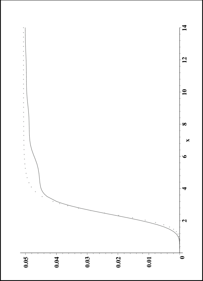
FIG. 1.: Plot of the exact $D(x)$ against its approximated form (dotted curve) in the range $0<x<14$

E The factorization approximation

To numerically perform the integrals needed to do obtain the spectrum it is useful to note the approximate factorization property

$$F(x,y)\approx F\left({x+y\over 2},{x+y\over 2}\right)\;G\left(\frac{x-y}{2}\right).$$ (149)

That is: to a good approximation $F(x,y)$ is given by its value along the nearest part of the diagonal, multiplied by a universal function of the distance away from the diagonal. A little experimental curve fitting is actually enough to show that to a good approximation

$$F(x,y)\approx D\left({x+y\over 2}\right)\;{\sin^{2}(3[x-y]/4)\over(3[x-y]/4)^{2}}.$$ (150)

From the plot we show below it is easy to check that the function $F(x,y)$ is quite well approximated by this factorized form. We feel important to stress that this is approximation is based on numerical experimentation, and is not an analytically-driven approximation. (In the infinite volume case we know that $F(x,y)\to(constant)\times\delta(x-y)$. The effect of finite volume is effectively to “smear out” the delta function. In this regard, it is interesting to observe that the combination $\sin^{2}(x)/(\pi x^{2})$ is one of the standard approximations to the delta function.) Our approximation is quite good everywhere except for values of $x$ and $y$ near the origin (less than 1) where the contribution of the function to the integral is very small.

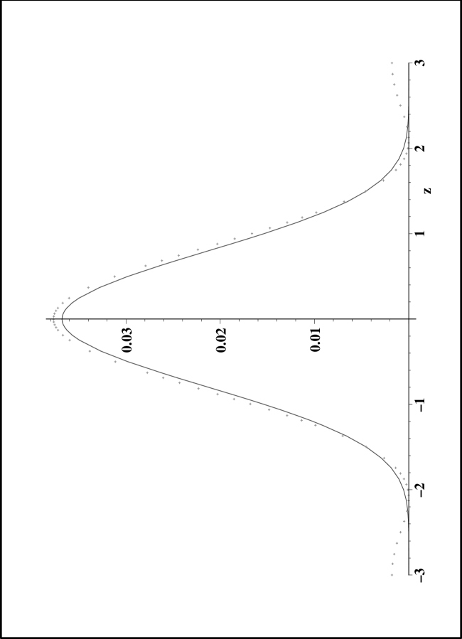
FIG. 2.: Transverse fit: An orthogonal slice of $F(x,y)$ intersecting the diagonal at $(x,y)=(3,3)$. Here $F(3+z,3-z)$ is plotted in comparison with $[\sin^{2}(3z/2)]/(3z/2)^{2}$. The solid line is the function, and the dotted line the analytic approximation

F The spectrum: numerical evaluation

We have now transformed the function $F(x,y)$ into an easy to handle product of two functions

$$F(x,y)\approx\frac{1}{2\pi^{2}}\frac{(x+y)^{6}}{16000+(x+y)^{6}}{\sin^{2}(3[x-y]/4)\over(3[x-y]/4)^{2}}.$$ (151)

We exhibit tridimensional graphs for both the exact (apart from the approximation of truncating the sum at a finite $l$) and approximate forms of the function $F(x,y)$. We have chosen the case of $R=500\;{\rm nm}$ (corresponding to $y_{*}=15\;n_{\mathrm{g}as}^{\mathrm{o}ut}/n_{\mathrm{l}iquid}$ as previously explained).

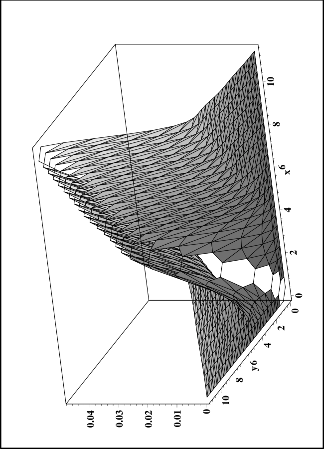
FIG. 3.: Plot of the exact $F(x,y)$ in the range $0<x<12$, $0<y<12$. The jagged behaviour along the diagonal is a numerical artifact, as the function is known to be smooth there.

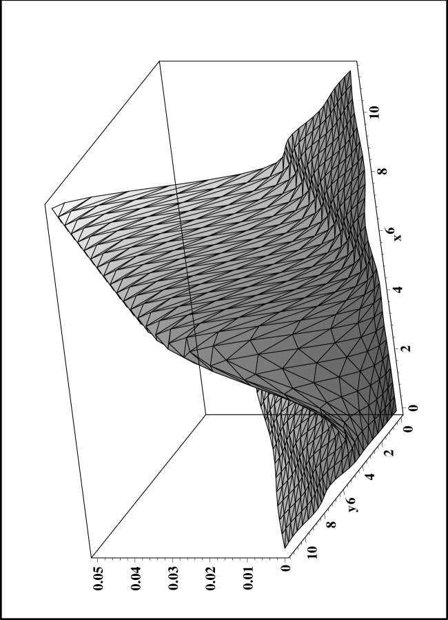
FIG. 4.: Plot of the approximated $F(x,y)$ in the range $0<x<12$, $0<y<12$

The dimensionless spectrum, based on equations (83) and (110), is

$${dN\over dx}=\frac{(n_{\mathrm{g}as}^{\mathrm{i}n}-n_{\mathrm{g}as}^{\mathrm{o}ut})^{2}}{2\;n_{\mathrm{g}as}^{\mathrm{i}n}n_{\mathrm{g}as}^{\mathrm{o}ut}}\int_{0}^{\infty}\left(\frac{n_{\mathrm{g}as}^{\mathrm{i}n}\,x^{2}+n_{\mathrm{g}as}^{\mathrm{o}ut}\,y^{2}}{n_{\mathrm{g}as}^{\mathrm{i}n}\,x+n_{\mathrm{g}as}^{\mathrm{o}ut}\,y}\right)^{2}D\left({x+y\over 2}\right){\sin^{2}(3[x-y]/4)\over(3[x-y]/4)^{2}}dy,$$ (152)

where $n_{\mathrm{g}as}^{\mathrm{o}ut}(x)$ and $n_{\mathrm{g}as}^{\mathrm{i}n}(y)$ are now the appropriate functions of $x$ and $y$ (See equations (132) and (131)). We have also manually inserted a factor $2$ to account for the photon polarizations.

As a consistency check, the infinite volume limit is equivalent to making the formal replacements

$${\sin^{2}(3[x-y]/4)\over(3[x-y]/4)^{2}}\to{4\pi\over 3}\delta(x-y),$$ (153)

and

$$D\left({x+y\over 2}\right)\to{1\over 2\pi^{2}}.$$ (154)

The first replacement can be formally justified as follows. It is known that a sequence of smooth functions approximating the delta function is given by

$$f_{s}(x)=\frac{1}{s\;\pi}\;\frac{\sin^{2}(s\;x)}{x^{2}};$$ (155)

indeed, one get

$$\lim_{s\to\infty}\;f_{s}(x)=\delta(x).$$ (156)

Then, it is straightforward to show that

$${\sin^{2}(3[x-y]/4)\over(3[x-y]/4)^{2}} = {\sin^{2}(R\;3[n_{\mathrm{g}as}^{\mathrm{i}n}\omega_{\mathrm{i}n}-n_{\mathrm{g}as}^{\mathrm{o}ut}\omega_{\mathrm{o}ut}]/(4c))\over(R\;3[n_{\mathrm{g}as}^{\mathrm{i}n}\omega_{\mathrm{i}n}-n_{\mathrm{g}as}^{\mathrm{o}ut}\omega_{\mathrm{o}ut}]/(4c))^{2}}$$ (157)

$$\to \frac{\pi}{R}\;\delta(\pi[n_{\mathrm{g}as}^{\mathrm{i}n}\omega_{\mathrm{i}n}-n_{\mathrm{g}as}^{\mathrm{o}ut}\omega_{\mathrm{o}ut}]/(4c))$$ (158)

$$= {4\pi\over 3}\;\delta(x-y).$$ (159)

Doing so, equation (152) reduces to the spectrum obtained for homogeneous dielectrics in [6]. Indeed

$${dN\over dx}={1\over 3\pi}\frac{(n_{\mathrm{g}as}^{\mathrm{i}n}-n_{\mathrm{g}as}^{\mathrm{o}ut})^{2}}{n_{\mathrm{g}as}^{\mathrm{i}n}n_{\mathrm{g}as}^{\mathrm{o}ut}}\;x^{2}\;\Theta(x_{*}-x).$$ (160)

With these consistency checks out of the way, it is now possible to perform the integral with respect to $y$ to estimate the spectrum for finite volume, and similarly to perform appropriate double integrals with respect to $x$ and $y$ to estimate both total photon production and average photon energy. In our companion paper [6] we showed that in the infinite volume limit there were two continuous branches of values for $n_{\mathrm{g}as}^{\mathrm{i}n}$ and $n_{\mathrm{g}as}^{\mathrm{o}ut}$ that led to approximately one million emitted photons with an average photon energy of $3/4$ the cutoff energy. If we now place the same values of refractive index into the formula (152) derived above, numerical integration again yields approximately one million photons with an average photon energy of $3/4$ times the cutoff energy. The total number of photons is changed by at worst a few percent, while the average photon energy is almost unaffected. (Some specific sample values are reported in Table I.) The basic result is this: as expected [6], finite volume effects do not greatly modify the results estimated by using the infinite volume limit. Note that $\hbar\Omega_{\mathrm{m}ax}$ is approximately $4$ eV, so that average photon energy in this crude model is about $3$ eV.

$\;n_{\mathrm{g}as}^{\mathrm{i}n}\;$	$\;n_{\mathrm{g}as}^{\mathrm{o}ut}\;$	Number of photons	$\langle E\rangle/\hbar\Omega_{\mathrm{m}ax}$
$2\times 10^{4}$	$1$	$1.06\times 10^{6}$	$0.803$
$71$	$25$	$1.00\times 10^{6}$	$0.750$
$68$	$34$	$1.06\times 10^{6}$	$0.751$
$9$	$25$	$0.955\times 10^{6}$	$0.750$
$1$	$12$	$0.98\times 10^{6}$	$0.765$

Table I: Some typical cases.

In addition, for the specific case $n_{\mathrm{g}as}^{\mathrm{i}n}=2\times 10^{4}$, $n_{\mathrm{g}as}^{\mathrm{o}ut}=1$, we have calculated and plotted the form of the spectrum. We find that the major result of including finite volume effects is to smear out the otherwise sharp cutoff coming from Schwinger’s step-function model for the refractive index. Other choices of refractive index lead to qualitatively similar spectra. These results are in reasonable agreement (given the simplicity of the present model) with experimental data.

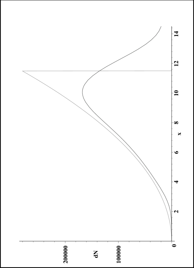
FIG. 5.: Spectrum $dN/dx$ obtained by integrating the approximated Bogolubov coefficient. We integrate from $y=0$ to $y_{*}=11.5$ and plot the resulting spectrum from $x=0$ to $x=14.5$. For $n_{\mathrm{o}ut}=1$ and $R=500$nm the relation between the non-dimensional quantitiy $x$ and the frequency $\nu$ is $x\sim\nu\cdot 10.5\cdot 10^{-15}$s. So $x\approx 11.5$ corresponds to $\nu\approx 1.1$ PHz. The curve with the sharp cutoff is the infinite volume approximation. Finite volume effects tend to smear out the sharp discontinuity, but do not greatly affect the total number of photons emitted.

V Discussion

The present paper presents calculations of the Bogolubov coefficients relating the two QED vacuum states appropriate to changes in the refractive index of a dielectric bubble. We have verified by explicit computation that photons are produced by rapid changes in the refractive index, and are in agreement with Schwinger in that QED vacuum effects remain a viable candidate for explaining SL. However, some details of the particular model considered in the present paper are somewhat different from that originally envisaged by Schwinger. Based largely on the fact that efficient photon production requires timescales of the order of femtoseconds we were led to consider rapid changes in the refractive index as the gas bubble bounces off the van der Waals hard core. It is important to realize that the speed of sound in the gas bubble can become relativistic at this stage [6].

We feel that theoretical computations along these lines have now been pushed as far as is meaningful given the current experimental situation. We have now constrained Casimir-like mechanisms for sonoluminescence into a relatively small region of parameter space, and it is experiment, rather than theory, that is likely to lead to further advances. We argue, both here and elsewhere, that Casimir-like mechanisms are viable, that they make both qualitative [21] and quantitative predictions, and that they are now sufficiently well defined to be experimentally falsifiable. (Possible extensions of the model will require much more detailed condensed matter information, such as experimental data regarding the actual refractive index inside the bubble as a function of time, space, and frequency.)

In conclusion, the present calculation (limited though it may be) represents an important advance: There now can be no doubt that changes in the refractive index of the gas inside the bubble lead to production of real photons—the controversial issues now move to quantitative ones of precise fitting of the observed experimental data. We are hopeful that more detailed models and data fitting will provide better explanations of the details of the SL effect.

A Generalizing the inner product

For the differential equation

$$\epsilon\;\partial_{0}(\partial_{0}E)-\nabla^{2}E=0,$$ (A1)

it is a standard exercise to write down a density and flux,

$$\rho=\epsilon\left(E_{1}^{*}\;\partial_{t}E_{2}-E_{2}\;\partial_{t}E_{1}^{*}\right),$$ (A2)

$$j=E_{1}^{*}\nabla E_{2}-E_{2}\nabla E^{*}_{1},$$ (A3)

and to then show that, by virtue of the differential equation (A1), these quantities satisfy a continuity equation

$$\partial_{t}\rho-\nabla\cdot j=0.$$ (A4)

Suppose now one has two solutions of the differential equation (A1), one can then define an inner product

$$(E_{1},E_{2})=-i\;\epsilon\int_{t}\left(E^{*}_{1}\partial_{t}E_{2}-E_{2}\partial_{t}E_{1}^{*}\right),$$ (A5)

where the integral is taken over a constant-time spacelike hypersurface. By virtue of the above, this inner product is independent of the time $t$ at which it is evaluated.

Now what happens if the dielectric is allowed to depend on both space and time? First the differential equation of interest is generalized to

$$\partial_{0}(\epsilon(x,t)\partial_{0}E)-\nabla^{2}E=0.$$ (A6)

Second, the density and flux become,

$$\rho=\epsilon(r,t)\left(E_{1}^{*}\partial_{t}E_{2}-E_{2}\partial_{t}E_{1}^{*}\right),$$ (A7)

$$j=E_{1}^{*}\nabla E_{2}-E_{2}\nabla E_{1}^{*}.$$ (A8)

By virtue of the differential equation (A6),

$$\partial_{t}\rho \equiv E_{1}^{*}\;\partial_{t}(\epsilon(x,t)\partial_{t}E_{2})-E_{2}\;\partial_{t}(\epsilon(x,t)\partial_{t}E_{1}^{*})$$ (A9)

$$= E_{1}^{*}\nabla^{2}E_{2}-E_{2}\nabla^{2}E_{1}^{*}$$ (A10)

$$= \nabla\cdot(E_{1}^{*}\nabla E_{2}-E_{2}\nabla E_{1}^{*})$$ (A11)

$$= \nabla\cdot j.$$ (A12)

Which implies that these generalized quantities satisfy a continuity equation

$$\partial_{t}\rho-\nabla\cdot j=0.$$ (A13)

This implies that the generalized inner-product [for two solutions $E_{1}$ and $E_{2}$ of the equation (A6) for time-dependent and space-dependent dielectric constants] must be

$$(E_{1},E_{2})=-{i\over 2}\int_{t}\epsilon(x,t)\left(E^{*}_{1}\partial_{t}E_{2}-E_{2}\partial_{t}E_{1}^{*}\right).$$ (A14)

By the continuity equation this inner product is independent of the time $t$ at which the integral is evaluated [provided of course, that $E_{1}$ and $E_{2}$ both satisfy (A6)]. This construction can be made completely relativistic. Define a four-vector $J^{\mu}$ by

$$J^{\mu}\equiv(\rho;j^{i}).$$ (A15)

Then for any edgeless achronal spacelike hypersurface $\Sigma$ there is a conserved inner product

$$(E_{1},E_{2})=-i\;\int_{\Sigma}\epsilon(x,t)\;J^{\mu}\;d\Sigma_{\mu}.$$ (A16)

B Some Bessel function identities

The inversion formula for Hankel Integral transforms is [26, 27]

$$\int_{0}^{\infty}r\;dr\;J_{\nu}(\kappa_{1}r)\;J_{\nu}(\kappa_{2}r)={\delta(\kappa_{1}-\kappa_{2})\over\sqrt{\kappa_{1}\;\kappa_{2}}}=2\;{\delta(\kappa_{1}-\kappa_{2})\over(\kappa_{1}+\kappa_{2})}=2\;\delta(\kappa_{1}^{2}-\kappa_{2}^{2}),$$ (B1)

this result being valid for $Re(\nu)>-{\textstyle{1\over 2}}$, and $\lambda_{(1,2)}>0$. On the other hand, another well-known standard result is

$$\int_{0}^{R}rdrJ_{\nu}(\kappa_{1}r)J_{\nu}(\kappa_{2}r)={R\left[\kappa_{1}J_{\nu}^{\prime}(\kappa_{1}R)J_{\nu}(\kappa_{2}R)-\kappa_{2}J_{\nu}(\kappa_{1}R)J_{\nu}^{\prime}(\kappa_{2}R)\right]\over\kappa_{2}^{2}-\kappa_{1}^{2}}$$ (B2)

(See, for instance (24.88) on page 142 of Spiegel [30]. Cf. also [28], formula 11.3.29 on page 484. This is of course a special case of the more general pseudo-Wronskian analysis presented in the text.) This is enough to imply

$$\lim_{R\to\infty}{R\left[\kappa_{1}J_{\nu}^{\prime}(\kappa_{1}R)J_{\nu}(\kappa_{2}R)-\kappa_{2}J_{\nu}(\kappa_{1}R)J_{\nu}^{\prime}(\kappa_{2}R)\right]\over\kappa_{2}^{2}-\kappa_{1}^{2}}={\delta(\kappa_{1}-\kappa_{2})\over\sqrt{\kappa_{1}\;\kappa_{2}}}$$ (B3)

By using the asymptotic forms of the Bessel functions (see, for example, equations (24.103)–(24.104) of Spiegel [30]) this is equivalent to the two spectral identities

$$\lim_{R\to\infty}{\sin(kR)\over k}=\pi\;\delta(k),$$ (B4)

and

$$\lim_{R\to\infty}{\cos(kR)\over k}=0.$$ (B5)

These spectral identities, together with the known asymptotic forms of the Bessel functions, then let us generalize (B3) above to obtain both

$$\lim_{R\to\infty}{R\left[\kappa_{1}N_{\nu}^{\prime}(\kappa_{1}R)N_{\nu}(\kappa_{2}R)-\kappa_{2}N_{\nu}(\kappa_{1}R)N_{\nu}^{\prime}(\kappa_{2}R)\right]\over\kappa_{2}^{2}-\kappa_{1}^{2}}={\delta(\kappa_{1}-\kappa_{2})\over\sqrt{\kappa_{1}\;\kappa_{2}}},$$ (B6)

and

$$\lim_{R\to\infty}{R\left[\kappa_{1}J_{\nu}^{\prime}(\kappa_{1}R)N_{\nu}(\kappa_{2}R)-\kappa_{2}J_{\nu}(\kappa_{1}R)N_{\nu}^{\prime}(\kappa_{2}R)\right]\over\kappa_{2}^{2}-\kappa_{1}^{2}}=0.$$ (B7)

These are the key equations needed to complete the argument leading to the correct normalization of the static eigenmodes. [See equation (31).]

REFERENCES

• [1] E-mail: liberati@sissa.it
• [2] E-mail: visser@kiwi.wustl.edu
• [3] E-mail: belgiorno@mi.infn.it
• [4] E-mail: sciama@sissa.it
• [5] B.P. Barber, R.A. Hiller, R. Löfstedt, S.J. Putterman Phys. Rep. 281, 65-143 (1997).
• [6] S. Liberati, M. Visser, F. Belgiorno, and D.W. Sciama, Sonoluminescence as a QED vacuum effect. I: Physical Scenario, quant-ph/9904013.
• [7] J. Schwinger, Proc. Nat. Acad. Sci. 89, 4091–4093 (1992).
• [8] J. Schwinger, Proc. Nat. Acad. Sci. 89, 11118–11120 (1992).
• [9] J. Schwinger, Proc. Nat. Acad. Sci. 90, 958–959 (1993).
• [10] J. Schwinger, Proc. Nat. Acad. Sci. 90, 2105–2106 (1993).
• [11] J. Schwinger, Proc. Nat. Acad. Sci. 90, 4505–4507 (1993).
• [12] J. Schwinger, Proc. Nat. Acad. Sci. 90, 7285–7287 (1993).
• [13] J. Schwinger, Proc. Nat. Acad. Sci. 91, 6473–6475 (1994).
• [14] C. Eberlein, Sonoluminescence as quantum vacuum radiation, Phys. Rev. Lett. 76, 3842 (1996). quant-ph 9506023
• [15] C. Eberlein, Theory of quantum radiation observed as sonoluminescence, Phys. Rev. A 53, 2772 (1996). quant-ph 9506024
• [16] C. Eberlein, Sonoluminescence as quantum vacuum radiation (replies to comments), Phys. Rev. Lett. 77, 4961 (1996); 78, 2269 (1997). quant-ph/9610034
• [17] C.S. Unnikrishnan and S. Mukhopadhyay, Phys. Rev. Lett. 77, 4960 (1996).
A. Lambrecht, M-T. Jaekel, and S. Reynaud, Phys. Rev. Lett. 78, 2267 (1997).
N. García and A.P. Levanyuk, Phys. Rev. Lett. 78, 2268 (1997).
• [18] S. Liberati, M. Visser, F. Belgiorno, and D.W. Sciama, Sonoluminescence: Bogolubov coefficients for the QED vacuum of a collapsing bubble, quant-ph/9805023.
• [19] S. Liberati, M. Visser, F. Belgiorno, and D.W. Sciama, Sonoluminescence as a QED vacuum effect, quant-ph/9805031.
• [20] S. Liberati, M. Visser, F. Belgiorno, and D.W. Sciama, Sonoluminescence and the QED vacuum, quant-ph/9904008.
• [21] F. Belgiorno, S. Liberati, M. Visser, and D.W. Sciama, Sonoluminescence: Two-photon correlations as a test for thermality, quant-ph/9904018.
• [22] C. E. Carlson, C. Molina–París, J. Pérez–Mercader, and M. Visser, Phys. Lett. B 395, 76-82 (1997). hep-th/9609195
• [23] C. E. Carlson, C. Molina–París, J. Pérez–Mercader, and M. Visser, Phys. Rev. D56, 1262 (1997). hep-th/9702007.
• [24] C. Molina–París and M. Visser, Phys. Rev. D56, 6629 (1997). hep-th/9707073
• [25] J. Holzfuss, M. Rüggeberg, and A. Billo, Phys. Rev. Lett. 81, 5434 (1998).
• [26] H. Bateman, Higher Transcendental Functions, Vol II, (McGraw-Hill, New York, 1953); See especially equation (8.1.1) on page 5.
• [27] J.D. Jackson, Classical Electrodynamics, (Wiley, New York, 1975); see equation (3.112) on page 110.
• [28] M. Abramowitz and I.A. Stegun, Handbook of Mathematical Functions, (Dover, New York, 1965).
• [29] A. Jeffrey, Handbook of Mathematical Formulas and Integrals, page 219, (Academic Press, San Diego, 1995).
• [30] M. Spiegel, Mathematical handbook of formulas and tables, (McGraw–Hill, New York, 1968).