Quantum gates with neutral atoms: Controlling collisional interactions in time dependent traps

Abstract

We theoretically study specific schemes for performing a fundamental two–qubit quantum gate via controlled atomic collisions by switching microscopic potentials. In particular we calculate the fidelity of a gate operation for a configuration where a potential barrier between two atoms is instantaneously removed and restored after a certain time. Possible implementations could be based on microtraps created by magnetic and electric fields, or potentials induced by laser light.

I Introduction

The creation and manipulation of many–particle entangled states offers new perspectives for the investigation of fundamental questions of quantum mechanics, and is the basis of applications such as quantum information processing. Several proposals to implement quantum logic [1] have been made including ion-traps [2], cavity QED and photons [3], and molecules in the context of NMR [4]. Very recently, we have identified a new way of entangling neutral atoms by using cold controlled collisions [5] (see also [6]). Neutral atoms are good candidates for quantum information processing, since they suffer a comparatively weak dissipative coupling to the environment. Techniques to cool and trap atoms by means of magnetic and optical potentials have been developed in the context of laser cooling and trapping, and Bose–Einstein condensation (BEC) [7]. In particular the ongoing development of magnetic microtraps [8] offers an interesting new perspective for storing and manipulating arrays of atoms [9, 10] and possible applications in quantum information [11].

Motivated by these new experimental possibilities we will study in this paper specific configurations of atoms stored in time dependent microtraps. We will assume that two internal states of the atoms $|a\rangle$ and $|b\rangle$ represent the logical states $|0\rangle$ and $|1\rangle$ of a qubit, respectively. The aim is to implement a fundamental two–qubit quantum gate between two atoms with the truth table

$$|0\rangle|0\rangle \rightarrow |0\rangle|0\rangle,$$ (1)

$$|0\rangle|1\rangle \rightarrow |0\rangle|1\rangle,$$ (2)

$$|1\rangle|0\rangle \rightarrow |1\rangle|0\rangle,$$ (3)

$$|1\rangle|1\rangle \rightarrow -|1\rangle|1\rangle,$$ (4)

by switching the trapping parameters. Eq. (4) represents a so called phase gate. To realize this transformation we will consider state selective switching of the trapping potential such that the atoms pick up a phase due to collisional interaction [12] only if they are in state $|b\rangle$. This can be achieved by raising and lowering a potential barrier between the two atoms as shown in Fig. 1. According to Fig. 1a the potential is initially composed of two separated wells. Ideally the atoms have been cooled to the vibrational ground states of the two wells. At time $t=0$ the shape of the trapping potential is changed for particles in state $|b\rangle$ (dashed line in Fig. 1b) while the potentials for the atoms in the state $|a\rangle$ remains unchanged (solid line in Fig. 1b). By removing the barrier the particles in state $|b\rangle$ start to oscillate and will collide.

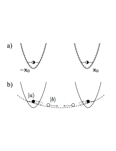
FIG. 1.: Configuration at times $t<0$, $t>\tau$ (a) and during the gate operation (b). The solid (dashed) curves show the potentials for particles in the internal state $|a\rangle$ ($|b\rangle$).

The “cold” collision represents a coherent interaction described by a pseudo–potential with a strength proportional to the $s$–wave scattering length [5]. This results in a phase shift of the wave function for both atoms in the internal state $|b\rangle$. The size of the phase shift can be controlled by the number of oscillations and the effective collisional interaction strength (see Sec. II A). As a last step the atoms have to be restored to the motional ground state of the trapping potential of Fig. 1a. This whole process of switching the potentials can be performed either as (i) switching the shape of the potential instantaneously at times $t=0$ and $t=\tau$ where $\tau$ is a multiple of the oscillation period in the well of Fig. 1b (dashed line), or, (ii) deforming the shape of the potential between Fig. 1a and b adiabatically. The aim of the present paper is to investigate the gate dynamics for the scenario (i), when the switching is instantaneous: In particular we are interested in the required physical parameters and the corresponding fidelities characterising the quality of the phase gate. We will also study the dependence of the fidelity on the temperature of the atoms. The paper is organized as follows. Section II describes the model and derives an expression for the collisional phase shift. In Sec. III we study the gate dynamics for the case of instantaneous switching while in Sec. IV we present numerical results for the fidelity.

II Model

In the present section we will write down the Hamiltonian for two interacting particles trapped in conservative time dependent potentials and derive an expression for the collisional phase shift.

A Hamiltonian

The dynamics of atoms in a time–varying, state–dependent trapping potential $V_{\alpha}({\bf x},t)$ (where $t$ is time and ${\bf x}\equiv(x,y,z)$ is the three-dimensional coordinate) can be described by the Hamiltonian operator

$$H = \sum_{\alpha\in\{a,b\}}\int d^{3}x\;\hat{\Psi}^{\dagger}_{\alpha}({\bf x})\left[-\frac{\hbar^{2}}{2m}{\bf\nabla}^{2}+V_{\alpha}({\bf x},t)\right]\hat{\Psi}_{\alpha}({\bf x})$$ (7)

$$\mbox{}+\sum_{\alpha,\beta\in\{a,b\}}\frac{1}{2}\int d^{3}x\,d^{3}x^{\prime}\,\hat{\Psi}^{\dagger}_{\alpha}({\bf x})\hat{\Psi}^{\dagger}_{\beta}({\bf x}^{\prime})$$

$$\qquad\qquad\qquad\mbox{}\times U_{\alpha\beta}({\bf x},{\bf x}^{\prime})\hat{\Psi}_{\beta}({\bf x}^{\prime})\hat{\Psi}_{\alpha}({\bf x}),$$

where $m$ is the mass of the atoms, $\hat{\Psi}_{\alpha}({\bf x})$ is a field operator for atoms in internal state $|\alpha\rangle$, and $U_{\alpha\beta}({\bf x},{\bf x}^{\prime})$ is the potential for the interaction between two atoms in states $|\alpha\rangle$ and $|\beta\rangle$, where $\alpha,\beta\in\{a,b\}$. We take a trapping potential of the form

$$V_{\alpha}({\bf x},t)=v_{\alpha}(x,t)+v_{\perp}(y)+v_{\perp}(z),$$ (8)

i.e. we assume the same shape along $y$ and $z$, which is independent of time and of the internal state.

For cold atoms the dominant collisional interaction is the $s$–wave scattering term described by a contact potential of the form

$$U_{\alpha\beta}({\bf x},{\bf x}^{\prime})=\frac{4\pi a_{s}^{\alpha\beta}\hbar^{2}}{m}\;\delta^{3}({\bf x}-{\bf x}^{\prime}),$$ (9)

where $a_{s}^{\alpha\beta}$ is the $s$–wave scattering length for the corresponding internal states. Note that for identical atoms in the same internal state $s$–wave scattering is only possible for bosonic atoms (cf. the $b$–$b$ collision in Fig. 1b). We therefore require, in the following, the field operators $\hat{\Psi}_{\alpha}({\bf x})$ to describe bosonic atoms and to obey the usual bosonic commutation relations.

Furthermore, we assume much stronger confinement along the $y$ and $z$ directions than in $x$, so that the probability of transverse excitations can be neglected. If each atom is initially in the ground state $|\psi_{\perp}\rangle$ of the transverse potentials, it will then remain in that state to a good approximation and the corresponding degrees of freedom can be integrated out. In this case the dynamics becomes effectively one–dimensional and is described by the Hamiltonian operator

$$H_{x} = \sum_{\alpha\in\{a,b\}}\int dx\;\hat{\psi}^{\dagger}_{\alpha}(x)\left[-\frac{\hbar^{2}}{2m}\frac{d^{2}}{dx^{2}}+v_{\alpha}(x,t)\right]\hat{\psi}_{\alpha}(x)$$ (12)

$$\mbox{}+\sum_{\alpha,\beta\in\{a,b\}}\frac{1}{2}\int dx\,dx^{\prime}\,\hat{\psi}^{\dagger}_{\alpha}(x)\hat{\psi}^{\dagger}_{\beta}(x^{\prime})$$

$$\qquad\qquad\qquad\mbox{}\times u_{\alpha\beta}(x-x^{\prime})\hat{\psi}_{\beta}(x^{\prime})\hat{\psi}_{\alpha}(x).$$

Here $\hat{\psi}_{\alpha}(x)$ is the one–dimensional analogue of $\hat{\Psi}_{\alpha}({\bf x})$, and

$$u_{\alpha\beta}(x-x^{\prime}) = \int dy\,dy^{\prime}\,dz\,dz^{\prime}\,U_{\alpha\beta}({\bf x},{\bf x}^{\prime})$$ (14)

$$\quad\times\left|\psi_{\perp}(y)\psi_{\perp}(y^{\prime})\psi_{\perp}(z)\psi_{\perp}(z^{\prime})\right|^{2}$$

$$= \frac{4\pi a_{s}\hbar^{2}}{m}\delta(x-x^{\prime})\left[\int dy|\psi_{\perp}(y)|^{4}\right]^{2},$$ (15)

is an effective interaction potential taking into account the transverse confinement of the atoms. The $\psi_{\perp}$ are the ground–state wavefunctions in the transverse directions (having energy $\hbar\omega_{\perp}/2$ each). Their time evolution will just contribute an overall phase factor (with a phase proportional to $\omega_{\perp}$), irrelevant for the quantities we are going to compute. We see that the effective interaction strength can be adjusted by changing the trapping parameters.

Eq. (12) holds for an arbitrary number of atoms. We now consider the case of two bosonic atoms 1 and 2, with internal states $|a\rangle_{1,2}$ and $|b\rangle_{1,2}$. Their evolution is governed by the first–quantized Hamiltonian

$${\cal H}=\sum_{\alpha,\beta\in\{a,b\}}{\cal H}_{\alpha\beta}\otimes|\alpha\rangle_{1}\langle\alpha|\otimes|\beta\rangle_{2}\langle\beta|,$$ (16)

where

$${\cal H}_{\alpha\beta} \equiv {\cal H}_{\alpha\beta}^{0}+u_{\alpha\beta},$$ (18)

$${\cal H}^{0}_{\alpha\beta} = {\cal H}_{\alpha}(p_{1},x_{1},t)+{\cal H}_{\beta}(p_{2},x_{2},t),$$ (19)

$${\cal H}_{\alpha}(p_{i},x_{i},t) = \frac{p_{i}^{2}}{2m}+v_{\alpha}(x_{i},t).$$ (20)

Here $x_{i}$ and $p_{i}$ are the position and momentum operator for particle $i=1,2$ respectively.

B Phase shift due to interaction

We call $|\psi_{\alpha\beta}^{(0)}(t)\rangle$ and $|\psi_{\alpha\beta}(t)\rangle$ the two–particle states at time $t$ evolved from the same initial state $|\psi_{\alpha\beta}(0)\rangle$ in the absence and in the presence of interaction, respectively:

$$i\hbar\partial_{t}|\psi^{(0)}_{\alpha\beta}(t)\rangle = {\cal H}^{0}_{\alpha\beta}|\psi^{(0)}_{\alpha\beta}(t)\rangle,$$ (22)

$$i\hbar\partial_{t}|\psi_{\alpha\beta}(t)\rangle = {\cal H}_{\alpha\beta}|\psi_{\alpha\beta}(t)\rangle.$$ (23)

We also define the overlaps

$$O_{0}(\psi_{\alpha\beta},t) \equiv \langle\psi_{\alpha\beta}(t)|\psi_{\alpha\beta}^{(0)}(t)\rangle;$$ (25)

$$O(\psi_{\alpha\beta},t) \equiv \langle\psi_{\alpha\beta}(t)|\psi_{\alpha\beta}(0)\rangle.$$ (26)

The condition that both atoms end up at time $t=\tau$ with the same spatial distribution they had at the beginning will not be exactly fulfilled in realistic situations. However, in order for our scheme to work it is required that this is true at least approximately:

$$|O(\psi_{\alpha\beta},\tau)|\approx 1\qquad\forall\;\alpha,\beta,$$ (27)

i.e. the two–atom final state should differ from the initial one just by a phase factor $\Phi_{\alpha\beta}(\tau)\equiv\arg[O(\psi_{\alpha\beta},\tau)]$:

$$|\psi_{\alpha\beta}(\tau)\rangle\approx e^{-i\Phi_{\alpha\beta}(\tau)}|\psi_{\alpha\beta}(0)\rangle.$$ (28)

We also assume that the interaction between atoms does not induce any significant alteration in the shape of the wave functions, i.e.

$$|O_{0}(\psi_{\alpha\beta},t)|\approx 1\qquad\forall\;\alpha,\beta,t.$$ (29)

Hence

$$|\psi_{\alpha\beta}(t)\rangle\approx e^{-i\phi_{\alpha\beta}(t)}|\psi_{\alpha\beta}^{(0)}(t)\rangle,$$ (30)

having defined the collisional phase

$$\phi_{\alpha\beta}(t)\equiv\arg[O_{0}(\psi_{\alpha\beta},t)],$$ (31)

accounting for the contribution of the interaction to the total phase $\Phi_{\alpha\beta}(\tau)$. The rest of the phase comes from the motion of the particles in the time–dependent trapping potential. From Eqs. (27) and (29) it follows that

$$|O(\psi^{(0)}_{\alpha\beta},\tau)|\approx 1\qquad\forall\;\alpha,\beta,$$ (32)

which implies, by analogy with Eq. (28),

$$|\psi_{\alpha\beta}^{(0)}(\tau)\rangle\approx e^{-i[\phi_{\alpha}(\tau)+\phi_{\beta}(\tau)]}|\psi_{\alpha\beta}(0)\rangle.$$ (33)

Here the kinematic phase $\phi_{\alpha}(\tau)$ [$\phi_{\beta}(\tau)$] is defined as the phase that one atom would acquire after evolving for a time $\tau$ in the potential $v_{\alpha}$ [$v_{\beta}$] in the absence of the other particle. By substituting Eq. (33) into Eq. (30) evaluated at $t=\tau$, and comparing it with Eq. (28), the collisional phase can be reexpressed as

$$\phi_{\alpha\beta}(\tau)\approx\Phi_{\alpha\beta}(\tau)-[\phi_{\alpha}(\tau)+\phi_{\beta}(\tau)].$$ (34)

By combining Eqs. (II B), (29) and (30), we find

$$\hbar\partial_{t}\phi_{\alpha\beta}(t)\approx\langle\psi^{(0)}_{\alpha\beta}(t)|u_{\alpha\beta}|\psi^{(0)}_{\alpha\beta}(t)\rangle\equiv\Delta E_{\alpha\beta}(t),$$ (35)

which is precisely the result one would expect from perturbation theory. In order for Eq. (29) to hold, the time–dependent energy shift defined in Eq. (35) has to satisfy the condition $\Delta E_{\alpha\beta}(t)\ll\hbar\omega$, with $\hbar\omega$ the first excitation energy of the system. Integration of Eq. (35) gives a perturbative expression for the collisional phase:

$$\phi_{\alpha\beta}(t)\approx\frac{1}{\hbar}\int_{0}^{t}dt^{\prime}\,\Delta E_{\alpha\beta}(t^{\prime}).$$ (36)

III Gate operation

To proceed further, we have to specify the functional form of the potential $v_{\alpha}(x,t)$ in Eq. (8). The two atoms are initially trapped along $x$ in two separate harmonic wells of frequency $\omega_{0}$, centered at $\pm x_{0}$. In order to simplify the analytic calculations, the confinement in the transverse directions is also assumed to be harmonic. At $t=0$ the barrier between the wells is suddenly removed in a selective way for atoms in internal state $|b\rangle$: an atom in state $\left|a\right\rangle$ feels no change, whereas one in state $\left|b\right\rangle$ finds itself in a new harmonic potential, centered on $x=0$ with frequency $\omega<\omega_{0}$. The atoms are allowed to oscillate for some time, and then at $t=\tau$ the barrier is suddenly raised again to trap them at the original positions. During this process the atoms acquire a kinematic phase due to their oscillations within the wells, and also – if they collide – an interaction phase due to the collision. Here we calculate these phases and consider the appropriate switching time $\tau$ for a quantum gate. In Sect. IV we make a quantitative estimate of the gate fidelity.

A Switching potential

We take the potential in Eq. (8) to be explicitly

$$v_{a}(x,t) = \frac{m\omega_{0}^{2}}{2}\bigl{[}\theta(x)(x-x_{0})^{2}+\theta(-x)(x+x_{0})^{2}\bigr{]};$$ (38)

$$v_{b}(x,t) = \left\{\begin{array}[]{ll}v_{a}(x,t)&t<0,\;t>\tau;\\ \displaystyle{\frac{m\omega^{2}}{2}x^{2}}&0\leq t\leq\tau;\end{array}\right.$$ (41)

$$v_{\perp}(y) = \frac{m\omega_{\perp}^{2}}{2}y^{2},$$ (42)

as shown in Fig. 1. As long as the single-well ground-state width $a_{0}=\sqrt{\hbar/m\omega_{0}}$ satisfies $a_{0}^{2}\ll x_{0}^{2}$ and there are no significant excitations to higher levels of $v_{a}(x,t)$, the actual behavior of that potential around the origin does not really matter and we can use Eq. (38) regardless of the experimental shape of the barrier around $x=0$. The ground state wavefunctions $\psi_{\pm}(x)$ of the right and left well of the potential $v_{a}(x,t)$ are given by

$$\psi_{\pm}(x) = \left(\frac{m\omega_{0}}{2\pi\hbar}\right)^{\frac{1}{4}}e^{-\frac{m\omega_{0}}{2\hbar}\left(x_{0}\mp x\right)^{2}},$$ (43)

while the ground state wavefunction in the transverse directions is given by

$$\psi_{\perp}(y) = \left(\frac{m\omega_{\perp}}{2\pi\hbar}\right)^{\frac{1}{4}}e^{-\frac{m\omega_{\perp}}{2\hbar}y^{2}}.$$ (44)

By assumption the overlap between the two wavefunctions $\psi_{+}(x)$ and $\psi_{-}(x)$ is negligible since the two particles are kept separated from each other in the potential $v_{a}(x,t)$. At $t=0$, the central barrier between the two wells is selectively switched off for state $|b\rangle$. A particle in this state will start moving towards the other atom along $x$ and an interaction will take place. We shall separately study the evolution of the system at $t\geq 0$ for each combination of internal states $(\alpha,\beta)$. For operation of the quantum gate analyzed here, it is important that $v_{b}(x,t)$ be accurately harmonic while $0\leq t\leq\tau$.

B Particles in the same internal state

1 Initial state

If both particles are in the same internal state $\left|\alpha\right\rangle$, this factorizes from the motional degrees of freedom and the initial state is

$$|\psi_{\alpha\alpha}(0)\rangle=\frac{|\psi_{-}\rangle|\psi_{+}\rangle+|\psi_{+}\rangle|\psi_{-}\rangle}{\sqrt{2}}\otimes|\alpha\rangle|\alpha\rangle.$$ (45)

The calculation can be simplified by introducing the center of mass (CM) and relative coordinates for the $x$–motion, thus rewriting

$$\psi_{\alpha\alpha}(x_{1},x_{2},0) \equiv \frac{1}{\sqrt{2}}\left[\psi_{-}(x_{1})\psi_{+}(x_{2})+\psi_{+}(x_{1})\psi_{-}(x_{2})\right]$$ (46)

$$= \psi_{\rm CM}(R,0)\psi_{\rm rel}(r,0),$$ (47)

where

$$\psi_{\rm CM}(R,0) = \left(\frac{M\omega_{0}}{\pi\hbar}\right)^{\frac{1}{4}}e^{-\frac{M\omega_{0}}{2\hbar}R^{2}},$$ (49)

$$\psi_{\rm rel}(r,0) = \left(\frac{\mu\omega_{0}}{4\pi\hbar}\right)^{\frac{1}{4}}\sum_{\varsigma=-1,+1}e^{-\frac{\mu\omega_{0}}{2\hbar}\left(2x_{0}+\varsigma r\right)^{2}},$$ (50)

with $M=2m$, $\mu=m/2$, $R=\left(x_{1}+x_{2}\right)/2$, $r=x_{2}-x_{1}$.

2 Time evolution

For $t\leq 0$, the particles are stored in the displaced wells and no interaction takes place. If both particles are in state $\left|a\right\rangle$, the potential remains unchanged also for $t\geq 0$; there is no collision and thus the collisional phase $\phi_{aa}=0$. The state simply picks up the phase due to the free evolution:

$$|\psi_{\alpha\alpha}(t)\rangle=e^{-i\omega_{0}t}|\psi_{\alpha\alpha}(0)\rangle.$$ (51)

We shall now consider the situation in which both particles are in state $\left|b\right\rangle$. In this case, after the barrier is switched off, the particles start oscillating in the harmonic trapping potential. In the absence of interaction they would come back to the initial state after an oscillation period $T_{\rm osc}=2\pi/\omega$, having acquired a phase $4\pi\omega_{\perp}/\omega$ because of the transverse confining potential. The interaction causes an additional phase to be accumulated by the wavefunction as the number of oscillations increases, and a slight decrease in the oscillation frequency, because the atoms acquire a small delay in their motion inside the trap as they come out from a collision. If the latter feature is not too strong, by choosing a switching time $\tau\approx 2N\pi/\omega$ it should be possible to get back the original state plus an interaction phase, that is adjusted to $\pm\pi$ by a proper choice of the trap parameters and of the number of collisions occurring during the actual gate operation, i.e. for $0<t<\tau$. We shall therefore focus on the dynamics in this time interval.

In the center of mass–relative coordinate system we get

$${\cal H}_{bb}=\frac{P^{2}}{2M}+\frac{M\omega^{2}}{2}R^{2}+\frac{p^{2}}{2\mu}+\frac{\mu\omega^{2}}{2}r^{2}+u_{bb}\left(r\right),$$ (52)

where $P=p_{1}+p_{2}$, $p=\left(p_{1}-p_{2}\right)/2$. If the interaction is neglected we can solve the two–particle Schrödinger equation for Hamiltonian Eq. (52) analytically as shown in Appendix A 1. It can be seen from Eqs. (A1-A12) that the unperturbed two-atom motion has a period of $T_{\rm osc}/2$ instead of $T_{\rm osc}$. This happens because the initial state, symmetric with respect to the origin, has nonzero projection only on the even eigenstates, having energies $(2n+1/2)\hbar\omega$: therefore, after a time $\pi/\omega$, each component of the wavefunction gets the same constant phase $\exp[i(2n+1/2)\pi]=\exp(i\pi/2)$. This has a simple physical interpretation: if the atoms do not interact, after half an oscillation period each particle is at its turning point, coinciding with the other atom’s starting location; so at that time the two atoms have interchanged their positions, but since they are indistinguishable this has to be regarded as exactly the same motional state they had at the beginning (apart from a phase factor).

When we take into account the interaction between particles, the center of mass motion is unaffected but the relative motion can no longer be treated analytically. The numerical method we use to carry out this calculation is outlined in Appendix A 2 a. It is, however, possible to take the interaction into account perturbatively as shown in the following section.

3 Perturbative calculation of the phase shift

Eqs. (14) and (44) combine to yield

$$u_{\alpha\beta}(x_{1}-x_{2})=2a_{s}^{\alpha\beta}\hbar\omega_{\perp}\delta(x_{1}-x_{2}).$$ (53)

When both particles are in state $|b\rangle$, the time–dependent energy shift defined in Eq. (35) can be calculated analytically:

$$\Delta E_{bb}(t) = \int dRdr|\psi_{CM}(R,t)\psi^{(0)}_{\rm rel}(r,t)|^{2}u_{bb}(r)$$ (54)

$$= a_{s}^{bb}\hbar\omega_{\perp}\sqrt{\frac{8m\Omega(t)}{\pi\hbar}}e^{-\frac{2m\omega_{0}}{\hbar}x_{0}^{2}\left[1-\sin^{2}(\omega t)\frac{\omega_{0}\Omega(t)}{\omega^{2}}\right]},$$ (55)

where $\Omega(t)$ is defined in Eq. (A2). The corresponding interaction-induced phase shift accumulated after an oscillation period is

$$\phi_{bb}(T_{\rm osc})\approx\frac{4a_{s}^{bb}\omega_{\perp}}{\sqrt{x_{0}^{2}\omega^{2}-a_{0}^{2}\omega_{0}^{2}/4}},$$ (56)

which has been evaluated by means of the well-known saddle–point approximation.

C Particles in different internal states

1 Initial state

When the internal states of the atoms are different, they no longer factorize as in Eq. (45) and the initial state is given by

$$\left|\psi_{ab}(0)\right\rangle=\frac{1}{\sqrt{2}}\left[|\psi_{-}\rangle_{1}|\psi_{+}\rangle_{2}\otimes|a\rangle_{1}|b\rangle_{2}+(1\leftrightarrow 2)\right],$$ (57)

where without loss of generality we assumed that the particle in the left (right) well is in internal state $|a\rangle$ ($|b\rangle$).

2 Time evolution

The relevant quantities can again be expressed in terms of the projection of the evolved state on the initial one. By virtue of symmetry under particle interchange, this turns out to be

$$O(\psi_{ab},t)=\langle\psi_{-}|\langle\psi_{+}|e^{-\frac{i}{\hbar}{\cal H}_{ab}t}|\psi_{-}\rangle|\psi_{+}\rangle.$$ (58)

Therefore we can restrict our analysis, as in the previous case, to the one–dimensional motion, starting from the non–symmetrized wavefunction $\psi_{-}(x_{1})\psi_{+}(x_{2})$. The Hamiltonian for $0<t<\tau$ reads

$${\cal H}_{ab} = \frac{p_{1}^{2}}{2m}+\frac{p_{2}^{2}}{2m}+\frac{m\omega_{0}^{2}}{2}\left(x_{1}+x_{0}\right)^{2}+\frac{m\omega^{2}}{2}x_{2}^{2}$$ (60)

$$\quad\mbox{}+u_{ab}(x_{1}-x_{2})$$

$$= \frac{P^{2}}{2M}+\frac{p^{2}}{2\mu}+\frac{m}{2}(\omega^{2}-\omega_{0}^{2})Rr+\frac{m}{2}\omega_{0}^{2}x_{0}^{2}\left(1-\frac{\omega_{0}^{2}}{\tilde{\omega}^{2}}\right)$$ (63)

$$\quad\mbox{}+\frac{M}{2}\tilde{\omega}^{2}\left(R+\frac{\omega_{0}^{2}}{2\tilde{\omega}^{2}}x_{0}\right)^{2}+\frac{\mu}{2}\tilde{\omega}^{2}\left(r-\frac{\omega_{0}^{2}}{\tilde{\omega}^{2}}x_{0}\right)^{2}$$

$$\quad\mbox{}+u_{ab}(r)$$

where $\tilde{\omega}\equiv\sqrt{\left(\omega^{2}+\omega_{0}^{2}\right)/2}$. Only the left well of $v_{a}(x_{1},t)$ has been considered since the wavefunction remains negligible in the region $x_{1}>0$ for $t>0$, as it is at $t=0$. It can be seen from Eq. (60) that the center of mass no longer decouples from the relative motion, unlike in the previous symmetrical case. A numerical calculation is needed to evaluate the phase shift $\phi_{ab}$. This is done in Appendix A 2 b.

D Particles at finite temperature

Up to now we have assumed the particles to be in a well known motional state. In realistic experimental situations this may not be the case. The temperature $T$ of the particles in the trap will be different from $0$ and thus the initial state of the system with particles in internal states $\alpha$, $\beta$ is given by the density operator

$$\rho_{\alpha\beta}(T,t=0^{-})\propto\mbox{e}^{-{\cal H}_{\alpha\beta}(0^{-})/k_{B}T}.$$ (64)

This takes the average over different initial excited states, with a thermal probability distribution corresponding to $T$. As shown in Appendix B the collisional phase accumulated is independent of the shape of the wave function if the particles move at a constant velocity with respect to each other and the shape of the one particle wavefunction does not change during the interaction. This is a good approximation for the interaction between particles in the same internal state $|b\rangle$. The particles interact in the vicinity of the center of the well where their velocity $v\approx x_{0}\omega$ is almost constant and the shape of the one particle wavefunction does not change substantially as long as the conditions

$$a_{x}\ll x_{0},\qquad\mbox{and}\qquad a\ll x_{0}$$ (65)

hold, where $a$ is the width of the one particle wavefunction when the particles cross the center of the trap and $a_{x}=\sqrt{\hbar/m\omega}$. Therefore the collisional phase $\phi_{bb}(T_{\rm osc})$ is almost independent of the temperature $T$ as long as mainly excitations fulfilling conditions Eq. (65) are populated. Note that we are neglecting transverse excitations. If all three motional degrees of freedom are characterized by the same temperature $T$, this is realistic as long as the condition $k_{B}T\ll\hbar\omega_{\perp}$ is satisfied. However, in principle it is also possible to cool the transverse motion separately, allowing a higher temperature along $x$. Of course this would require that the rethermalization time is much larger than the experimental time scale. This lack of sensitivity to temperature applies quite generally, for example to atoms interacting in an optical lattice as discussed in [5], provided that the velocity at which the atoms are made to interact (in that case the velocity of lattice movements) is kept constant during the interaction.

IV A physical implementation

We now consider the implementation of a switching potential by means of static electric and magnetic trapping forces. We first discuss the possibility of obtaining the desired state dependence by means of devices which are experimentally available [9, 11], when the present magnetic devices can be combined with nanofabricated electrodes. Then we compute the performance of a quantum gate for realistic trapping parameters.

A Microscopic electromagnetic trapping potential

The interaction between the magnetic dipole moment of an atom in some hyperfine state $|F,m_{F}\rangle$ and an external static magnetic field ${\bf B}$ entails an energy $U_{\rm magn}\approx g_{F}\mu_{B}m_{F}|{\bf B}|$ depending on the atomic internal state via the quantum number $m_{F}$ (here $\mu_{B}$ is the Bohr magneton and $g_{F}$ is the Landé factor). The Stark shift induced on an atom by an electric field ${\bf E}$ gives an energy (independent on the hyperfine sublevel) $U_{\rm el}\approx\frac{1}{2}\alpha_{\rm el}|{\bf E}|^{2}$, where $\alpha_{\rm el}$ is the atomic polarizability. The interplay between these two effects can be exploited in order to obtain a trapping potential whose shape depends on the internal state of the atoms. As an example, we consider an atomic mirror like the one recently realized [9] from a conventional video tape with sinusoidal magnetization ${\bf M}=(M_{0}\cos[k_{M}x],0,0)$ along the $x$–axis. The period of the pattern, $2\pi/k_{M}$, can be as small as $1\mu$m with the system studied in [9], or even close to 100 nm using existing magnetic storage technologies. In order to get a microscopic trapping potential [11], it is necessary to apply an external bias field ${\bf B}^{\rm ext}\equiv(0,B^{\rm ext}_{y},B^{\rm ext}_{z})$, oriented mainly along the $z$ axis, normal to the mirror’s surface, and with a small component along $y$ in order to prevent trap losses due to spin flips occurring at magnetic field zeros. In this case the magnetic trapping potential is

$$V_{m_{F}}({\bf x}) = g_{F}\mu_{B}m_{F}\Big{\{}B_{0}^{2}e^{-2k_{M}z}\cos^{2}(k_{M}x)+(B^{\rm ext}_{y})^{2}$$ (67)

$$\quad+\left[B_{0}e^{-k_{M}z}\sin(k_{M}x)+B^{\rm ext}_{z}\right]^{2}\Big{\}}^{\frac{1}{2}},$$

where $B_{0}=\mu_{0}M_{0}(1-e^{-k_{M}\delta})/2$ and $\delta$ is the tape thickness. The minima of $V_{m_{F}}$ form a periodic pattern above the tape surface, at a height $z_{0}=\ln(\mu_{0}M_{0}/B_{0})/k_{M}$ typically of the order of some fractions of $\mu$m. The spacing between two nearest minima along $x$ is just the period of the magnetization, $2\pi/k_{M}$. With present-day technology, trapping frequencies can range from a few tens of kHz up to some MHz. Microscopic electrodes can be nanofabricated on the mirror’s surface [10], thus allowing for the design of a potential with the characteristics described in Sect. III.

For the states $|a\rangle$ and $|b\rangle$ we choose the hyperfine structure states $|a\rangle\equiv|F=1,m_{F}=-1\rangle$ and $|b\rangle\equiv|F=2,m_{F}=2\rangle$ of the $5S_{1/2}$ level of ⁸⁷Rb, having scattering lengths $a_{s}^{bb}\approx a_{s}^{ab}\approx 5.1$ nm. Several schemes of loading atoms into the trap have been envisaged (see for example [9, 11]). Most of them rely on an intermediate step, where atoms can be trapped and cooled without coming in contact with the magnetic mirror. This pre–loading stage can be either a magnetic trap initially displaced from the surface, or a different kind of trap (for instance an evanescent wave mirror, where different internal states can be trapped by gravity close to the surface [13] before the atoms are put in the correct states for magnetic trapping), to be replaced by the electromagnetic microtrap with a gradual switch–on of the electric and bias magnetic fields in the final stage of loading [10]. This could also allow for implementing a controlled filling of the trap sites by adiabatically turning on the periodic potential, in a similar way to that discussed in [14].

B Results

1 Time evolution during gate operation

If both particles are in state $|a\rangle$, there is no interaction-induced phase shift, as expressed in Eq. (51). The results for both particles in state $|b\rangle$ are shown in Fig. 2a, while those for differing internal states appear in Fig. 2b. The harmonic potential ensures that the system comes periodically back to its initial state. In the absence of interaction, the frequency of recurrencies is twice as high for $|\psi_{bb}(t)\rangle$ as it is for $|\psi_{ab}(t)\rangle$, as already discussed at the end of Sect. III B 2. The interaction also makes the two cases substantially different from each other. Its effect on the atomic motion is not dramatic if both particles are in state $|b\rangle$: actually, the oscillation period in the presence of interaction is increased by only $\delta t\approx 1.4\times 10^{-3}T_{\rm osc}$ with the parameters used here. The collisional phase $\phi_{bb}$ increases in steps at the times $t_{k}\equiv(2k+1)T_{\rm osc}/4$, when the atoms meet at the center of the well, and remains constant at intermediate times while they are apart. Note that since the particles are indistinguishable the amplitude for the particles to bounce back during the colllision does not harm the perfomance of our scheme. The contributions of the reflected and the non-reflected part to the wavefunction are indistinguishable. What matters is whether of not the two–particle spatial distribution approaches the initial one, and this is satisfied to a high accuracy in our case.

The behavior is quite different if the atoms are in different internal states. The phase shift increases in larger steps since the collision is close to the turning point of the particle in state $|b\rangle$, near $x=x_{0}$. Here the velocity of the particle is much smaller than at the center of the trap and thus the interaction time is longer, allowing a larger phase to accumulate. The collision also excites vibrations of the particle in state $|a\rangle$. The resulting loss of energy from the particle in state $|b\rangle$ leads to a decreasing oscillation amplitude of that particle, and the initial state is no longer recovered. This problem can be avoided if the potential minimum for state $\left|a\right\rangle$ is displaced along the transverse direction from the one for state $\left|b\right\rangle$ by means of an additional electrostatic field [11], so that the atoms interact if and only if they are both in state $\left|b\right\rangle$.

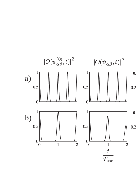
FIG. 2.: Dynamics during gate operation: projection of the initial state on the state evolved without (left) and with interaction (center); interaction–induced phase shift (right). Results are shown for different combinations of internal states: a) $\alpha=\beta=b$; b) $\alpha\not=\beta$. We choose $\omega=2\pi 17.23$ kHz and $\omega_{\perp}=2\pi 150$ kHz, corresponding to ground–state widths $a_{x}\approx 82$ nm, $a_{\perp}\approx 28$ nm, with the initial wells having frequency $\omega_{0}=2\omega$ and displaced by $x_{0}=5a_{x}$. Time is in units of the oscillation period $T_{\rm osc}$.

2 Gate fidelity at $T=0$

Ideally, the scheme described above should realize the mapping

$$|a\rangle|a\rangle \rightarrow e^{-i2\phi_{a}}|a\rangle|a\rangle,$$ (68)

$$|a\rangle|b\rangle \rightarrow e^{-i(\phi_{a}+\phi_{b}+\phi_{ab})}|a\rangle|b\rangle,$$ (69)

$$|b\rangle|a\rangle \rightarrow e^{-i(\phi_{b}+\phi_{a}+\phi_{ab})}|b\rangle|a\rangle,$$ (70)

$$|b\rangle|b\rangle \rightarrow e^{-i(\phi_{bb}+2\phi_{b})}|b\rangle|b\rangle,$$ (71)

where $\phi_{a}$ and $\phi_{b}$ are the phases due to the time evolution without taking into account the interaction. We assume, as above, that the trapping potential is designed to prevent the atoms interacting if they are in different internal states. Therefore we set $\phi_{ab}=0$ in Eq. (71) and consider only $\phi_{bb}$ in the following. We use the minimum fidelity $F$ [15] to characterize the quality of the gate. $F$ is defined as

$$F=\min_{\chi}{\bf\Bigl{(}}{\rm tr}_{\rm ext}\left\{\langle\tilde{\chi}|{\cal U}S\left[|\chi\rangle\langle\chi|\otimes\rho_{0}\right]S^{\dagger}{\cal U}^{\dagger}|\tilde{\chi}\rangle\right\}{\bf\Bigr{)}},$$ (72)

where $|\chi\rangle$ is an arbitrary internal state of both atoms, and $|\tilde{\chi}\rangle$ is the state resulting from $|\chi\rangle$ using the mapping (71). The trace is taken over properly symmetrized motional states, ${\cal U}$ is the evolution operator for the internal states coupled to the external motion (including the collision), $S$ represents symmetrization under particle interchange and $\rho_{0}$ is the density operator for the initial two–particle motional ground state. A straightforward calculation gives

$$F\!=\!\textstyle{\frac{1}{2}\frac{1-A^{2}-B^{2}[(1+A^{2})B^{2}-4ABC+2C^{2}]\cos^{2}(\phi_{bb})}{(1+A)\{2+B[(1-A)B+2C]\cos(\phi_{bb})\}-B^{2}(B-C)^{2}\cos^{2}(\phi_{bb})}}$$ (73)

where $A=\bigl{|}O(\psi_{bb}^{(0)},\tau)\bigr{|}^{\frac{1}{2}}$, $B=|O(\psi_{bb},\tau)|^{\frac{1}{2}}$, $C=\bigl{|}O_{0}(\psi_{bb},\tau)\bigr{|}^{\frac{1}{2}}$. With the parameters quoted above, we obtain $F\approx 0.99$ either by choosing a gate operating time $\tau=7(T_{\rm osc}+\delta t)$, maximizing $B$, or $\tau=7T_{\rm osc}$, maximizing instead $A$. We prefer this latter choice since, after a time $\tau=NT_{\rm osc}=2N\pi/\omega$, the $j^{\rm th}$ component of the $x$–wavefunction of an atom in state $|b\rangle$ in the basis of eigenstates of $v_{b}(0\leq t\leq\tau)$ gets a phase $2N(j+1/2)\pi$ (here $N=7$). This brings some simplifications: e.g., the kinematic phases can be written as

$$\phi_{a}=N\pi\frac{\omega_{0}+2\omega_{\perp}}{\omega},\qquad\phi_{b}=N\pi\frac{\omega+2\omega_{\perp}}{\omega}.$$ (74)

The general form of $\phi_{b}$ is much more complicated. Fig. 3a shows that after 7 complete oscillations Eq. (31) yields a phase shift $\phi_{bb}(7T_{\rm osc})\approx\pi$ due to the interaction, whereas the perturbative formula Eq. (56) gives $7\phi_{bb}(T_{\rm osc})\approx 0.97\pi$. The figure also shows that the overlap $|O_{0}(\psi_{bb},t)\bigr{|}$ remains close to 1, satisfying Eq. (29). The curve has local minima at the times $t_{k}$ defined in Sect. IV B 1, signalling that a collision is taking place, and shows a global decrease due to the accumulating delay of the interacting motion with respect to the noninteracting one. The fidelity turns out to be

$$F=\frac{1}{2}\left\{1-\bigl{|}O_{0}(\psi_{bb},\tau)\bigr{|}\cos\left[\phi_{bb}(\tau)\right]\right\}.$$ (75)

3 Gate fidelity at $T\not=0$

In order to compute the temperature dependence $F(T)$ of the fidelity, the density matrix for the motional degrees of freedom in Eq. (72) has to be replaced by

$$\rho_{\rm ext}(T)=\sum_{l,n}P_{ln}(T)|l\rangle_{R}\langle l|\otimes|n\rangle_{r}\langle n|,$$ (76)

which coincides with $\rho_{0}$ at $T=0$. Here we have introduced the eigenstates $|l\rangle_{R}$ for the center of mass and $|n\rangle_{r}$ for the relative motion. The probabilities $P_{ln}(T)$ for occupation of the CM and relative motion excited states are calculated assuming for each atom a thermal distribution corresponding to temperature $T$, as expressed by Eq. (64). We obtain

$$F(T)=\frac{1}{2}\Bigl{\{}1-\sum_{l,n}P_{ln}(T)\bigl{|}O_{0}(\psi_{(n)},\tau)\bigr{|}\cos\bigl{[}\phi_{(n)}(\tau)\bigr{]}\Bigr{\}},$$ (77)

where

$$\psi_{(n)}(r) = \left(\frac{m\omega_{0}}{2\pi\hbar}\right)^{\frac{1}{4}}\sum_{\varsigma=-1,+1}\frac{e^{-\frac{m\omega_{0}}{4\hbar}\left(2x_{0}+\varsigma r\right)^{2}}}{\sqrt{n!2^{n+1}}}$$ (79)

$$\qquad\qquad\mbox{}\times H_{n}\left[\sqrt{\frac{m\omega_{0}}{2\hbar}}(2x_{0}+\varsigma r)\right].$$

In particular, $\psi_{(0)}\equiv\psi_{bb}$ and $\phi_{(0)}\equiv\phi_{bb}$. The corresponding interaction–induced phase shifts $\phi_{(n)}(t)$ are shown in Fig. 3b,c.

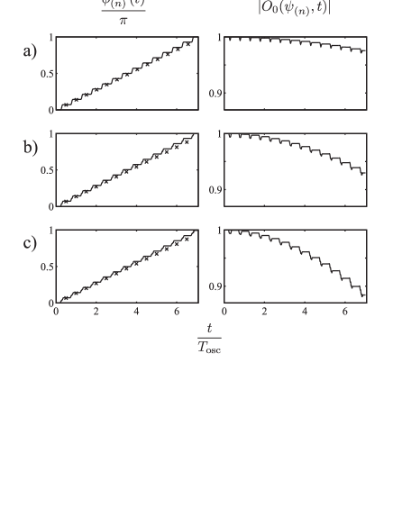
FIG. 3.: Dynamics for both atoms in state $\left|b\right\rangle$, with relative–motion excitations: a) $n=0$; b) $n=1$; c) $n=2$. On the left: interaction–induced phase shift; the crosses refer to the perturbative result from Eq. (36), explicitly given by Eq. (56) for $n=0$, and evaluated numerically for $n>0$. On the right: projection of the evolved state on the corresponding state evolved without interaction. Trap parameters have the same values as in Fig. 2 and satisfy Eq. (B11) since $a_{0}\omega_{0}/(4x_{0}\omega)=0.07$ in this case.

The discrepancy between the interacting and the noninteracting motion increases with $n$, but nevertheless the phase shift $\phi_{(n)}$ remains still close to $\pi$ (Fig. 3b and c), as already discussed in Sect. III B 3. Consequently the fidelity is not rapidly suppressed with temperature.

For example, one might well be interested in the values of $F(T)$ for temperatures up to $k_{B}T\approx\hbar\omega_{0}$. Let us therefore define $\gamma\equiv\exp(-\hbar\omega_{0}/k_{B}T)$ and neglect terms of $o(\gamma^{7})$ in the evaluation of Eq. (77) to obtain

$$F(T) \approx F(0)-\frac{1}{2}\sum_{n=1}^{6}\gamma^{n}\Bigl{\{}\bigl{|}O_{0}(\psi_{(n)},\tau)\bigr{|}\cos\left[\phi_{(n)}(\tau)\right]$$ (81)

$$\qquad\;\;\mbox{}-\bigl{|}O_{0}(\psi_{(n-1)},\tau)\bigr{|}\cos\left[\phi_{(n-1)}(\tau)\right]\Bigr{\}}.$$

This still gives a high fidelity $F(T)\approx 0.96$ even at $k_{B}T=2\hbar\omega_{0}$, for which $\gamma^{7}\approx 0.03$. We note that, in order to reach such a high fidelity, the timing has to be quite precise, with a resolution better than $10^{-3}T_{\rm osc}$ corresponding to tens of ns in this case.

V Conclusions

We have shown that entanglement among ultracold neutral atoms can be controlled by means of microscopic switching potentials. The fidelity for a fundamental two–qubit quantum gate turns out to be quite robust with respect to temperature: in fact, with the parameters quoted below Fig. 2, we find $F(T)\approx 0.96$ for $T\approx 3\mu$K in the $x$–motion, while assuming ground–state cooling in the transverse directions. We find a gate operation time of $\tau\approx 0.4$ms, over which coherence can probably be preserved with presently available experimental systems. Static microtraps based on available atomic mirrors [9, 11] provide a good opportunity for a first implementation of our scheme. Here nanofabrication technologies allow steep potentials to be achieved with small charges and/or currents. Trapping fields can be controlled electronically in a fast and accurate way [10].

Some problems remain to be addressed. To perform even a single gate operation, the trap should be loaded with exactly one atom per well. Read-out should be done possibly without removing atoms from the trap. In order to build up more complex operations, gates should be arranged in a periodic structure where coherent atom transport may take place between different locations. This would permit gate operations either on one pair of atoms at a time, or on several pairs in parallel, a fact which could be exploited for efficient implementation of quantum error correcting schemes and fault–tolerant quantum computing [16]. This will be the subject of future work.

A Time evolution

1 Analytical calculation

If both particles are in state $|b\rangle$ we start from the Hamiltonian Eq. (52), neglect the interaction term, and solve the Schrödinger equation. We find (omitting the internal state indices $bb$)

$$\psi_{\rm CM}(R,t)=\left[\frac{M\Omega(t)}{\pi\hbar}\right]^{\frac{1}{4}}e^{i\phi_{\rm CM}(R,t)-\frac{M\Omega(t)}{2\hbar}R^{2}},$$ (A1)

where

$$\Omega(t) = \frac{\omega^{2}\omega_{0}}{\left[\omega^{2}\cos^{2}(\omega t)+\omega_{0}^{2}\sin^{2}(\omega t)\right]},$$ (A2)

$$\phi_{\rm CM}(R,t) = \frac{M\Omega(t)}{2\hbar}\frac{\omega_{0}^{2}-\omega^{2}}{\omega_{0}\omega}R^{2}\cos(\omega t)\sin(\omega t)-\frac{\omega t}{2}$$ (A4)

$$-\frac{1}{2}{\rm arctan}\left[\frac{\left(\omega_{0}-\omega\right)\cos(\omega t)\sin(\omega t)}{\omega\cos^{2}(\omega t)+\omega_{0}\sin^{2}(\omega t)}\right].\!$$

From Eqs. (49) and (A1) it follows

$$\left|O\left(\psi_{\rm CM},t\right)\right|^{2}=\left[1+\frac{\left(\omega_{0}^{2}-\omega^{2}\right)^{2}}{4\omega_{0}^{2}\omega^{2}}\sin^{2}\left(\omega t\right)\right]^{-\frac{1}{2}}.$$ (A5)

If the particles did not interact, the relative motion would be

$$\psi_{\rm rel}^{(0)}(r,t) = \sqrt{\frac{\mu\Omega(t)}{4\pi\hbar}}\left(e^{i\phi_{\rm rel}(-r,t)-\frac{\mu\Omega(t)}{2\hbar}\left[r+2x_{0}\cos(\omega t)\right]^{2}}\right.$$ (A7)

$$\qquad\;\left.\mbox{}+e^{i\phi_{\rm rel}(r,t)-\frac{\mu\Omega(t)}{2\hbar}\left[r-2x_{0}\cos(\omega t)\right]^{2}}\right),$$

where

$$\phi_{\rm rel}(r,t) = \textstyle{-\frac{\omega t}{2}-\frac{1}{2}{\scriptstyle\arctan}\left[\frac{\left(\omega_{0}-\omega\right)\cos(\omega t)\sin(\omega t)}{\omega\cos^{2}(\omega t)+\omega_{0}\sin^{2}(\omega t)}\right]}$$ (A9)

$$\textstyle{+\frac{2\mu\Omega(t)}{\hbar\omega\omega_{0}}{\scriptstyle\sin(\omega t)}\left[\bigl{(}\frac{\omega_{0}^{2}-\omega^{2}}{4}{\scriptstyle r^{2}+\omega_{0}^{2}x_{0}^{2}}\bigr{)}{\scriptstyle\cos(\omega t)+\omega_{0}^{2}x_{0}r}\right]}.$$

The overlap between the states Eqs. (50) and (A7) is

$$\left|O\bigl{(}\psi_{\rm rel}^{(0)},t\bigr{)}\right|^{2} = \Biggl{(}e^{-\frac{8m\omega_{0}\omega^{2}x_{0}^{2}\cos^{2}(\omega t)}{\hbar\omega_{+}^{2}(t)}}+e^{-\frac{8m\omega_{0}\omega^{2}x_{0}^{2}\sin^{2}(\omega t)}{\hbar\omega_{-}^{2}(t)}}$$ (A12)

$$\quad\mbox{}+\frac{2\cos\left[\frac{4m\omega}{\hbar}\frac{\omega_{0}^{2}(\omega_{0}^{2}+\omega^{2})}{\omega_{+}^{2}(t)\omega_{-}^{2}(t)}{\scriptstyle x_{0}^{2}}\right]}{e^{\frac{4m\omega_{0}}{\hbar}\left[\frac{\cos^{2}(\omega t)}{\omega_{+}^{2}(t)}+\frac{\sin^{2}(\omega t)}{\omega_{-}^{2}(t)}\right]\omega^{2}x_{0}^{2}}}\Biggm{)}$$

$$\mbox{}\times\left[\textstyle{1+\frac{(\omega_{0}^{2}-\omega^{2})^{2}}{4\omega_{0}^{2}\omega^{2}}\sin^{2}\left(\omega t\right)}\right]^{-\frac{1}{2}}$$

with $\omega_{\pm}(t)=\sqrt{\omega^{2}+\omega_{0}^{2}\pm\left(\omega^{2}-\omega_{0}^{2}\right)\cos\left(\omega t\right)}$.

This result for the relative motion should be compared to the actual evolution in the presence of interaction, which cannot be computed analytically. If the particles are in different internal states we also have to resort to numerical methods.

2 Numerical calculation

a Particles in the same internal state

We write the state vector as a sum over the eigenstates $\left|n\right\rangle$ of a harmonic oscillator of mass $\mu$ and frequency $\omega$,

$$\left|\psi_{\rm rel}(t)\right\rangle=\sum_{n}e^{-i\left(n+1/2\right)\omega t}c_{n}(t)\left|n\right\rangle$$ (A13)

and approximate the potential by a truncated sum

$$\delta(r) \approx \sum_{k,l}^{N_{\rm max}}\left|k\right\rangle\left\langle k\right|\delta(r)\left|l\right\rangle\left\langle l\right|$$ (A14)

$$= \sum_{k,l}^{N_{\rm max}}\psi_{k}^{*}(0)\psi_{l}(0)|k\rangle\langle l|,$$ (A15)

where $\psi_{n}(x)=\left\langle x|n\right\rangle$. We have checked that the final result is independent of $N_{\rm max}$, with $N_{\rm max}$ of the order of some tens. The Schrödinger equation for $\left|\psi_{\rm rel}(t)\right\rangle$ gives

$$\dot{c}_{n}(t)=-i2a_{s}^{bb}\omega_{\perp}\psi_{n}^{*}(0)\sum_{l=0}^{N_{\rm max}}\psi_{l}(0)e^{i(n-l)\omega t}c_{l}(t),$$ (A16)

which we solve numerically for $c_{n}(t)$ with $0\leq n\leq N_{\rm max}$. The initial conditions, from Eq. (50), read

$$c_{n}(0) = \frac{e^{-\frac{m\omega_{0}\omega}{\hbar(\omega_{0}+\omega)}x_{0}^{2}}}{\sqrt{n!2^{n}}}\frac{(\omega_{0}\omega)^{\frac{1}{4}}}{\sqrt{\omega_{0}+\omega}}\left(\frac{\omega_{0}-\omega}{\omega_{0}+\omega}\right)^{\frac{n}{2}}$$ (A18)

$$\textstyle{\times\left[H_{n}\Bigl{(}\sqrt{\frac{2m\omega\omega_{0}^{2}x_{0}^{2}}{\hbar(\omega_{0}^{2}-\omega^{2})}}\Bigm{)}+H_{n}\Bigl{(}\sqrt{\frac{2m\omega\omega_{0}^{2}x_{0}^{2}}{\hbar(\omega^{2}-\omega_{0}^{2})}}\Bigm{)}\right]}.$$

b Particles in different internal states

In order to solve the Schrödinger equation for the Hamiltonian Eq. (60) we decompose the state vector

$$\left|\psi_{ab}(t)\right\rangle=\sum_{j,k}e^{-i\left(j+k+1\right)\tilde{\omega}t}c_{jk}(t)|\tilde{j}\rangle_{R}|\tilde{k}\rangle_{r},$$ (A19)

(where now $\tilde{\psi}_{j}(x)=\langle x|\tilde{j}\rangle$ are the eigenfunctions of a harmonic oscillator with frequency $\tilde{\omega}$ and mass $m$) and obtain for the coefficients

$$\dot{c}_{jk}(t)\! = i\frac{\tilde{\omega}(\omega_{0}^{2}-\omega^{2})}{2\left(\omega_{0}^{2}+\omega^{2}\right)}\Big{\{}c_{j+1,k+1}(t)e^{-i2\tilde{\omega}t}\sqrt{\left(j+1\right)\left(k+1\right)}$$ (A25)

$$\mbox{}+c_{j-1,k+1}(t)\sqrt{j\left(k+1\right)}+c_{j-1,k-1}(t)e^{i2\tilde{\omega}t}\sqrt{jk}$$

$$\mbox{}+c_{j+1,k-1}(t)\sqrt{\left(j+1\right)k}+\frac{m\tilde{\omega}}{\hbar}\frac{\omega^{2}-\omega_{0}^{2}}{\omega_{0}^{2}}\xi^{2}c_{jk}(t)$$

$$\mbox{}+\sqrt{\frac{2m\tilde{\omega}}{\hbar}}\xi\Big{[}e^{i\tilde{\omega}t}\big{(}c_{j-1,k}(t)\sqrt{j}-c_{j,k-1}(t)\sqrt{k}\big{)}$$

$$\mbox{}+e^{-i\tilde{\omega}t}\big{(}c_{j+1,k}(t)\sqrt{j+1}-c_{j,k+1}(t)\sqrt{k+1}\big{)}\Big{]}\Big{\}}$$

$$\mbox{}-i\sqrt{2}a_{s}^{ab}\omega_{\perp}\tilde{\psi}_{k}^{*}(-\xi)\sum_{l}\tilde{\psi}_{l}^{*}(-\xi)e^{i(k-l)\tilde{\omega}t}c_{jl}(t)$$

where $\xi=x_{0}\omega_{0}^{2}/\sqrt{2}\tilde{\omega}^{2}$.

This can again be solved numerically, starting from the initial conditions, derived from Eqs. (49), (50),

$$c_{jk}(0) = \frac{e^{-\frac{m\omega_{0}\omega(\xi^{2}+x_{0}^{2}-\sqrt{2}x_{0}\xi)}{\hbar(\omega_{0}+\omega)}}}{\sqrt{j!k!2^{j+k-2}}}\frac{\sqrt{\omega_{0}\omega}}{\omega_{0}+\omega}\Bigl{(}\frac{\omega_{0}-\omega}{\omega_{0}+\omega}\Bigr{)}^{\frac{j+k}{2}}\!$$ (A28)

$$\textstyle{\times\left[H_{j}\Bigl{(}\sqrt{\frac{m\omega\omega_{0}^{2}(\sqrt{2}x_{0}-\xi)^{2}}{\hbar(\omega_{0}^{2}-\omega^{2})}}\Bigr{)}+H_{k}\Bigl{(}\sqrt{\frac{m\omega\omega_{0}^{2}\xi^{2}}{\hbar(\omega_{0}^{2}-\omega^{2})}}\Bigr{)}\right]}.$$

B Interaction phase shift for excited initial states

Let us consider two bosonic atoms in the same internal state $|\alpha\rangle$, but in two different single–particle motional states $|\varphi_{-}\rangle$ and $|\varphi_{+}\rangle$ with vanishing overlap. The initial motional state has the form

$$|\varphi(0)\rangle=\frac{|\varphi_{-}\rangle|\varphi_{+}\rangle+|\varphi_{+}\rangle|\varphi_{-}\rangle}{\sqrt{2}}.$$ (B1)

We assume that: (i) the particles move against each other, come in contact during a certain time interval $[t_{i},t_{f}]$ and then separate again; (ii) the velocity of each particle and the shape of its wavefunction do not vary during the interaction. Thus for $t_{i}\leq t\leq t_{f}$ we write:

$$\langle x_{1}|\varphi_{-}(t)\rangle = \varphi^{\prime}(x_{1}-vt),$$ (B3)

$$\langle x_{2}|\varphi_{+}(t)\rangle = \varphi^{\prime\prime}(x_{2}+vt),$$ (B4)

where $v$ is a positive constant. It follows

$$\phi_{\alpha\alpha}(T_{\rm osc}) \approx \frac{1}{\hbar}\int_{t_{i}}^{t_{f}}dt\;\langle\varphi(t)|u_{\alpha\alpha}(x_{1},x_{2})|\varphi(t)\rangle$$ (B5)

$$= 4a_{s}^{\alpha\alpha}\omega_{\perp}\int_{t_{i}}^{t_{f}}dt\int_{-\infty}^{+\infty}dx_{1}$$ (B7)

$$\qquad\mbox{}\times\left|\varphi^{\prime}(x_{1}-vt)\right|^{2}\left|\varphi^{\prime\prime}(x_{1}+vt)\right|^{2}$$

$$\approx \frac{2a_{s}^{bb}\omega_{\perp}}{v}\int_{-\infty}^{+\infty}dx\,dy\,\left|\varphi^{\prime}(x)\right|^{2}\left|\varphi^{\prime\prime}(y)\right|^{2}$$ (B8)

$$= \frac{2a_{s}^{bb}\omega_{\perp}}{v},$$ (B9)

where a change of variables $x=x_{1}-vt$, $y=x_{1}+vt$ has been introduced, and the limits of integration in $t$ have been extended to $\pm\infty$ since the single–particle wavefunctions Eqs. (B3)-(B4) overlap just for a finite time. The result turns out to be independent of the initial state. We can compare it to Eq. (56), which was obtained in the harmonic potential Eq. (41) starting from the single–particle states $|\psi_{\pm}\rangle$ instead of $|\varphi_{\pm}\rangle$. In this case

$$v\equiv\left|\partial_{t}\langle\psi_{\pm}|e^{\frac{i}{\hbar}{\cal H}_{b}t}x\,e^{-\frac{i}{\hbar}{\cal H}_{b}t}|\psi_{\pm}\rangle\big{|}_{t=t_{k}}\right|=x_{0}\omega,$$ (B10)

and the atoms collide twice during one oscillation period. Therefore the collisional phase Eq. (56) should be twice as big as Eq. (B9). This is true provided that the maximum velocity for the atomic motion in the well $v_{b}(x,0\leq t\leq\tau)$ is large with respect to the analogous quantity for the ground–state motion in the wells $v_{a}(x,t)$, i.e. if

$$x_{0}\omega\gg a_{0}\omega_{0}/4.$$ (B11)

REFERENCES

• [1] For a review on quantum computing in general see, for example, A. M. Steane, Rept. Prog. Phys. 61, 117-173 (1998).
• [2] J. I. Cirac and P. Zoller, Phys. Rev. Lett. 74, 4091 (1995); Q. A. Turchette, C. S. Wood, B. E. King, C. J. Myatt, D. Leibfried, W. M. Itano, C. Monroe, and D. J. Wineland, ibid. 81 3631 (1998).
• [3] Q. A. Turchette, C. J. Hood, W. Lange, H. Mabuchi, and H. J. Kimble, Phys. Rev. Lett. 75, 4710 (1995); X. Maître, E. Hagley, G. Nogues, C. Wunderlich, P. Goy, M. Brune, J. M. Raimond, and S. Haroche, ibid. 79, 769 (1997); E. Hagley, X. Maître, G. Nogues, C. Wunderlich, M. Brune, J. M. Raimond, and S. Haroche, ibid. 79, 1 (1997); T. Pellizzari, S. A. Gardiner, J. I. Cirac, and P. Zoller, ibid. 75, 3788 (1995).
• [4] D. G. Cory, A. F. Fahmy, and T. F. Havel, Proc. Natl. Acad. Sci. USA 94, 1634 (1997); N. A. Gershenfeld, and I. L. Chuang, Science 275, 350 (1997).
• [5] D. Jaksch, H.–J. Briegel, J. I. Cirac, C. W. Gardiner, and P. Zoller, Phys. Rev. Lett. 82, 1975 (1999).
• [6] G. K. Brennen, C. M. Caves, P. S. Jessen, and I. H. Deutsch, Phys. Rev. Lett. 82, 1060 (1999).
• [7] M. H. Anderson, J. R. Ensher, M. R. Matthews, C. E. Wieman, and E. A. Cornell, Science, 269, 198 (1995). C. C. Bradley, C. A. Sackett, J. J. Tollett, and R. G. Hulet, Phys. Rev. Lett. 75, 1687 (1995). K. B. Davies, M.-O. Mewes, M. R. Andrews, N. J. van Druten, D. S. Durfee, D. M. Kurn, and W. Ketterle, ibid. 75, 3969 (1995). D. S. Hall, M. R. Matthews, C. E. Wieman, and E. A. Cornell, ibid. 81, 1543 (1998); 81, 4532 (1998). D. S. Hall, M. R. Matthews, J. R.Ensher, C. E. Wieman, and E. A. Cornell 1998, ibid. 81, 1539 (1998); 81, 4531 (1998). D. M. Stamper-Kurn, M. R. Andrews, A. P. Chikkatur, S. Inouye, H.-J. Miesner, J. Stenger, and W. Ketterle, ibid. 80, 2027 (1998).
• [8] J. Schmiedmayer in XVIII International Conference on Quantum Electronics: Technical Digest, edited by G. Magerl (Technische Universität Wien, Vienna 1992), Series 1992, Vol. 9, p.284 (1992); J. Schmiedmayer, Phys. Rev. A 52, R13 (1995); J. D. Weinstein, K. Libbrecht, Phys. Rev. A 52, 4004 (1995). V. Vuletic et al., Phys. Rev. Lett. 80, 1634 (1998); J. Fortagh et al., Phys. Rev. Lett. 81, 5310 (1998); J. Denschlag, D. Cassettari, J. Schmiedmayer, Phys. Rev. 82, 2014 (1998).
• [9] T. M. Roach, H. Abele, M. G. Boshier, H. L. Grossman, K. P. Zetie, and E. A. Hinds, Phys. Rev. Lett. 75, 629 (1995); E. A. Hinds, M. G. Boshier, and I. G. Hughes. ibid. 80, 645 (1998).
• [10] J. Schmiedmayer, Eur. Phys. J. D 4, 57 (1998).
• [11] E. A. Hinds, Phil. Trans. Roy. Soc. 357, 1 (1999)
• [12] This was measured for example in an atom interferometer: J. Schmiedmayer et al., Phys. Rev. Lett. 74, 1043 (1995).
• [13] Yu. B. Ovchinnikov, I. Manek, and R. Grimm, Phys. Rev. Lett. 79, 2225 (1997).
• [14] D. Jaksch, C. Bruder, J. I. Cirac, C. W. Gardiner, and P. Zoller, Phys. Rev. Lett. 81, 3108 (1998).
• [15] B. Schumacher, Phys. Rev. A 54, 2614 (1996).
• [16] H.–J. Briegel, T. Calarco, D. Jaksch, J. I. Cirac, and P. Zoller (submitted to J. Mod. Opt.).