Bogoliubov dispersion relation and the possibility of superfluidity for weakly-interacting photons in a 2D photon fluid

Abstract

The Bogoliubov dispersion relation for the elementary excitations of the weakly-interacting Bose gas is shown to hold for the case of the weakly-interacting photon gas (the “photon fluid”) in a nonlinear Fabry-Perot cavity. The chemical potential of a photon in the 2D photon fluid does not vanish. The Bogoliubov relation, which is also derived by means of a linearized fluctuation analysis in classical nonlinear optics, implies the possibility of a new, superfluid state of light. The theory underlying an experiment in progress to observe sound waves in the photon fluid is described, and another experiment to measure the critical velocity of this superfluid is proposed.

I Introduction

The quantum many-body problem, with its many, rich manifestations in condensed matter physics, has had a long and illustrious history. In particular, superconductivity and superfluidity were two major discoveries in this field. Although at present much is well understood (e.g., the BCS theory of superconductivity), the recent experimental discoveries of Bose-Einstein condensation in laser-cooled atoms [1, 2, 3, 4] raises new and interesting questions, such as whether the observed Bose-Einstein condensates are superfluids, or whether persistent currents can exist in these new states of matter.

Historically speaking, in the study of the interaction of light with matter, most of the emphasis has been on exploring new states of matter, such as the recently observed atomic Bose-Einstein condensates. However, not as much attention has been focused on exploring new states of light. Of course, the invention of the laser led to the discovery of a new state of light, namely the coherent state, which is a very robust one. Two decades ago, squeezed states were discovered, but these states are not as robust as the coherent state, since they are easily degraded by scattering and absorption. In contrast to the laser, which involves a system far away from equilibrium, we shall explore here states close to the ground state of a photonic system. Hence they should be robust ones.

Here we shall study the many-body problem by studying the interacting many-photon system (the “photon fluid”) near its ground state. In this paper we shall explore some theoretical considerations which suggest the possibility of a new state of light, namely, the superfluid state. In particular, we shall derive the Bogoliubov dispersion relation for the weakly-interacting photon gas with repulsive photon-photon interactions, starting both from the microscopic (i.e., second-quantized) level, and also from the macroscopic (i.e., classical-field) level. Thereby we shall find an expression for the effective chemical potential of a photon in the photon fluid, and shall relate the velocity of sound in the photon fluid to this nonvanishing chemical potential. In this way, we lay the theoretical foundations for an experiment in progress to measure the sound-wave-like dispersion relation for the photon fluid. We also propose another experiment to measure the critical velocity of this fluid, and thus to test for the possibility of the superfluidity of the resulting state of the light.

Although the interaction Hamiltonian used in this paper is equivalent to that used earlier in four-wave squeezing, we emphasize here the many-body, collective aspects of the problem which result from multiple photon-photon interactions. This leads to the idea of the “photon fluid.” Since the microscopic and macroscopic analyses yield the same Bogoliubov dispersion relation for excitations of this fluid, it may be argued that there is nothing fundamentally new in the microscopic analysis given below which is not already contained in the macroscopic, classical nonlinear optical analysis. However, it is the microscopic analysis which leads to the new, heuristic viewpoint of the interacting photon system as a “photon fluid,” a conception which could give rise to new ways of understanding and discovering nonlinear optical phenomena. Furthermore, the interesting question of the quantum optical state of the light inside the cavity resulting from multiple interactions between the photons (i.e., whether it results in a coherent, squeezed, Fock, or some other quantum state), cannot be addressed by classical nonlinear optical methods. Thus this paper represents a first attempt to formulate the new concept of a “photon fluid” starting from the microscopic viewpoint, and to lay the foundations for answering the question concerning the resulting quantum optical state of the light.

II The Bogoliubov problem

Here we re-examine one particular many-body problem, the one first solved by Bogoliubov [5, 6]. Suppose that one has a zero-temperature system of bosons which are interacting with each other repulsively, for example, a dilute system of small, bosonic hard spheres. Such a model was intended to describe superfluid helium, but in fact it did not work well there, since the interactions between atoms in superfluid helium were too strong for the theory for be valid. In order to make the problem tractable theoretically, let us assume that these interactions are weak. In the case of light, the interactions between the photons are in fact always weak, so that this assumption is a good one. However, these interactions are nonvanishing, as demonstrated by the fact that photon-photon collisions mediated by atoms excited near, but off, resonance have been experimentally observed [7]. We start with the Bogoliubov Hamiltonian

$$H = H_{free}+H_{int}$$ (1)

$$H_{free} = \sum_{p}\epsilon(p)a_{p}^{\dagger}a_{p}$$ (2)

$$H_{int} = \frac{1}{2}\sum_{\kappa pq}V(\kappa)a_{p+\kappa}^{\dagger}a_{q-\kappa}^{\dagger}a_{p}a_{q}\,,$$ (3)

where the operators $a_{p}^{\dagger}$ and $a_{p}$ are creation and annihilation operators, respectively, for bosons with momentum $p$, which satisfy the Bose commutation relations

$$[a_{p},a_{q}^{\dagger}]=\delta_{pq}\mbox{ and }[a_{p},a_{q}]=[a_{p}^{\dagger},a_{q}^{\dagger}]=0\,.$$ (4)

The first term $H_{free}$ in the Hamiltonian represents the energy of the free boson system, and the second term $H_{int}$ represents the energy of the interactions between the bosons arising from the potential energy $V(\kappa)$. The interaction term is equivalent to the one responsible for producing squeezed states of light via four-wave mixing [10]. It represents the annihilation of two particles, here photons, of momenta $p$ and $q$, along with the creation of two particles with momenta $p+\kappa$ and $q-\kappa$, in other words, a scattering process with a momentum transfer $\kappa$ between a pair of particles with initial momenta $p$ and $q$, along with the assignment of an energy $V(\kappa)$ to this scattering process.

III The free-photon dispersion relation inside a Fabry-Perot resonator

Photons with momenta $p$ and $q$ also obey the above commutations relations, so that the Bogoliubov theory should in principle also apply to the weakly-interacting photon gas. The factor $\epsilon(p)$ represents the energy as a function of the momentum (the dispersion relation) for the free, i.e., noninteracting, bosons. In the case of photons in a Fabry-Perot resonator, the boundary conditions of the mirrors cause the $\epsilon(p)$ of a photon trapped inside the resonator to correspond to an energy-momentum relation which is identical to that of a nonrelativistic particle with an effective mass [7, 8] of $m=\hbar\omega/c^{2}$. This can be understood starting from Fig. 1.

For high-reflectivity mirrors, the vanishing of the electric field at the reflecting surfaces of the mirrors imposes a quantization condition on the allowed values of the $z$-component of the photon wave vector, $k_{z}=n\pi/L$, where $n$ is an integer, and $L$ is the distance between the mirrors. Thus the usual frequency-wavevector relation

$$\omega(k)=c[k_{x}^{2}+k_{y}^{2}+k_{z}^{2}]^{1/2}\,,$$ (5)

upon multiplication by $\hbar$, becomes the energy-momentum relation for the photon

$$E(p)=c[p_{x}^{2}+p_{y}^{2}+p_{z}^{2}]^{1/2}=c[p_{x}^{2}+p_{y}^{2}+\hbar^{2}n^{2}\pi^{2}/L^{2}]^{1/2}=c[p_{x}^{2}+p_{y}^{2}+m^{2}c^{2}]^{1/2}\,,$$ (6)

where $m={\hbar}n\pi/Lc$ is the effective mass of the photon. In the limit of small-angle (or paraxial) propagation, where the small transverse momentum of the photon satisfies the inequality

$$p_{\perp}=[p_{x}^{2}+p_{y}^{2}]^{1/2}\ll p_{z}=\hbar k_{z}=\hbar n\pi/L\,,$$ (7)

we obtain from a Taylor expansion of the relativistic relation, a nonrelativistic energy-momentum relation for the 2D noninteracting photons inside the Fabry-Perot resonator

$$E(p_{\perp})\cong mc^{2}+p_{\perp}^{2}/2m\,,$$ (8)

where $m={\hbar}n\pi/Lc\cong\hbar\omega/c^{2}$ is the effective mass of the confined photons. It is convenient to redefine the zero of energy, so that only the effective kinetic energy,

$$\epsilon(p_{\perp})\cong p_{\perp}^{2}/2m\,,$$ (9)

remains. To establish the connection with the Bogoliubov Hamiltonian, we identify the two-dimensional momentum $p_{\perp}$ as the momentum $p$ that appears in this Hamiltonian, and the above $\epsilon(p_{\perp})$ as the $\epsilon(p)$ that appears in Eq. (3).

IV The Bogoliubov dispersion relation for the photon fluid

Now we know that in an ideal Bose gas at absolute zero temperature, there exists a Bose condensate consisting of a macroscopic number $N_{0}$ of particles occupying the zero-momentum state. This feature should survive in the case of the weakly-interacting Bose gas, since as the interaction vanishes, one should recover the Bose condensate state. Hence following Bogoliubov, we shall assume here that even in the presence of interactions, $N_{0}$ will remain a macroscopic number in the photon fluid[9]. This macroscopic number will be determined by the intensity of the incident laser beam which excites the Fabry-Perot cavity system, and turns out to be a very large number compared to unity (see below). For the ground state wave function $\Psi_{0}(N_{0})$ with $N_{0}$ particles in the Bose condensate in the $p=0$ state, the zero-momentum operators $a_{0}$ and $a_{0}^{\dagger}$ operating on the ground state obey the relations

$$a_{0}\left|\Psi_{0}(N_{0})\right> = \sqrt{N_{0}}\left|\Psi_{0}(N_{0}-1)\right>$$ (10)

$$a_{0}^{\dagger}\left|\Psi_{0}(N_{0})\right> = \sqrt{N_{0}+1}\left|\Psi_{0}(N_{0}+1)\right>\,.$$ (11)

Since $N_{0}\gg 1$, we shall neglect the difference between the factors $\sqrt{N_{0}+1}$ and $\sqrt{N_{0}}$. Thus one can replace all occurrences of $a_{0}$ and $a_{0}^{\dagger}$ by the $c$-number $\sqrt{N_{0}}$, so that to a good approximation $[a_{0},a_{0}^{\dagger}]\approx 0$. However, the number of particles in the system is then no longer exactly conserved, as can be seen by examination of the term in the Hamiltonian

$$\sum_{\kappa}V(\kappa)a_{\kappa}^{\dagger}a_{-\kappa}^{\dagger}a_{0}a_{0}\approx N_{0}\sum_{\kappa}V(\kappa)a_{\kappa}^{\dagger}a_{-\kappa}^{\dagger}\,,$$ (12)

which represents the creation of a pair of particles, i.e., photons, with momenta $\kappa$ and $-\kappa$ out of nothing.

However, whenever the system is open one, i.e., whenever it is connected to an external reservoir of particles which allows the total particle number number to fluctuate around some constant average value, then the total number of particles need only be conserved on the average. Formally, one standard way to compensate for the lack of exact particle number conservation is to use the Lagrange multiplier method and subtract a chemical potential term $\mu N_{op}$ from the Hamiltonian (just as in statistical mechanics when one goes from the canonical ensemble to the grand canonical ensemble) [11]

$$H\rightarrow H^{\prime}=H-\mu N_{op},$$ (13)

where $N_{op}=\sum_{p}a_{p}^{\dagger}a_{p}$ is the total number operator, and $\mu$ represents the chemical potential, i.e., the average energy for adding a particle to the open system described by $H$. In the present context, we are considering the case of a Fabry-Perot cavity with low, but finite, transmissivity mirrors which allow photons to enter and leave the cavity, due to an input light beam coming in from the left and an output beam leaving from the right. This permits a realistic physical implementation of the external reservoir, since the Fabry-Perot cavity allows the total particle number inside the cavity to fluctuate due to particle exchange with the beams outside the cavity. However, the photons remain trapped inside the cavity long enough so that a thermalized condition is achieved after many photon-photon interactions (i.e., after many collisions), thus allowing the formation of a photon fluid.

It will be useful to separate out the zero-momentum components of the interaction Hamiltonian, since it will turn out that there is a macroscopic occupation of the zero-momentum state due to Bose condensation. The prime on the sums $\sum^{\prime}_{p}$, $\sum^{\prime}_{p\kappa}$, and $\sum^{\prime}_{\kappa pq}$ in the following equation denotes sums over momenta explicitly excluding the zero-momentum state, i.e., all the running indices $p$, $\kappa$, $q$,$p+\kappa$,$q-\kappa$ which are not explicitly set equal to zero, are nonzero:

$$H_{int} = \frac{1}{2}V(0)a_{0}^{\dagger}a_{0}^{\dagger}a_{0}a_{0}+V(0){\sum_{p}}^{\prime}a_{p}^{\dagger}a_{p}a_{0}^{\dagger}a_{0}+$$ (16)

$${\sum_{p}}^{\prime}\left(V(p)a_{p}^{\dagger}a_{0}^{\dagger}a_{p}a_{0}+\frac{1}{2}\left[V(p)a_{p}^{\dagger}a_{-p}^{\dagger}a_{0}a_{0}+V(p)a_{0}^{\dagger}a_{0}^{\dagger}a_{p}a_{-p}\right]\right)+$$

$${\sum_{p\kappa}}^{\prime}V(\kappa)\left(a_{p+\kappa}^{\dagger}a_{0}^{\dagger}a_{p}a_{\kappa}+a_{p+\kappa}^{\dagger}a_{-\kappa}^{\dagger}a_{p}a_{0}\right)+\frac{1}{2}{\sum_{\kappa pq}}^{\prime}V(\kappa)\left(a_{p+\kappa}^{\dagger}a_{q-\kappa}^{\dagger}a_{p}a_{q}\right)\,.$$

Here we have also assumed that $V(p)=V(-p)$. By thus separating out the zero-momentum state from the sums in the Hamiltonian, and replacing all occurrences of $a_{0}$ and $a_{0}^{\dagger}$ by $\sqrt{N_{0}}$, we find that the Hamiltonian $H^{\prime}$ decomposes into three parts

$$H^{\prime}=H_{0}+H_{1}+H_{2}\,,$$ (17)

where

$$H_{0}=\frac{1}{2}V(0)a_{0}^{\dagger}a_{0}^{\dagger}a_{0}a_{0}\approx\frac{1}{2}V(0)N_{0}^{2}\,,$$ (18)

$$H_{1}\approx{\sum_{p}}^{\prime}\epsilon^{\prime}(p)a_{p}^{\dagger}a_{p}+\frac{1}{2}N_{0}{\sum_{p}}^{\prime}V(p)\left(a_{-p}^{\dagger}a_{p}^{\dagger}+a_{-p}a_{p}\right)\,,$$ (19)

$$H_{2}\approx\sqrt{N_{0}}\;{\sum_{p\kappa}}^{\prime}V(\kappa)\left(a_{p+\kappa}^{\dagger}a_{p}a_{\kappa}+a_{p+\kappa}^{\dagger}a_{-\kappa}^{\dagger}a_{p}\right)+\frac{1}{2}{\sum_{\kappa pq}}^{\prime}V(\kappa)\left(a_{p+\kappa}^{\dagger}a_{q-\kappa}^{\dagger}a_{p}a_{q}\right)\,,$$ (20)

where

$$\epsilon^{\prime}(p)=\epsilon(p)+N_{0}V(0)+N_{0}V(p)-\mu$$ (21)

is a modified photon energy, and where $N_{0}$ and $\mu$ are given by

$$N_{0}+<\Psi_{0}|{\sum_{p}}^{\prime}a_{p}^{\dagger}a_{p}|\Psi_{0}>=N\,$$ (22)

and

$$\mu=\frac{\partial E_{0}}{\partial N}\,.$$ (23)

Here $E_{0}=\left<\Psi_{0}|H|\Psi_{0}\right>$ is the ground state energy of $H$. In the approximation that there is little depletion of the Bose condensate due to interactions (i.e., $N\approx N_{0}\gg 1$), the first term of Eq. (16) (i.e., $H_{0}$ in Eq. (18)) dominates, so that

$$E_{0}\approx\frac{1}{2}N_{0}^{2}V(0)\approx\frac{1}{2}N^{2}V(0),$$ (24)

and therefore that

$$\mu\approx NV(0)\approx N_{0}V(0).$$ (25)

This implies that the effective chemical potential of a photon, i.e., the energy for adding a photon to the photon fluid, is given by the number of photons in the Bose condensate times the repulsive pairwise interaction energy between photons with zero relative momentum. It should be remarked that the fact that the chemical potential is nonvanishing here makes the thermodynamics of this two-dimensional photon system quite different from the usual three-dimensional, Planck blackbody photon system [12]. In the same approximation, Eq. (21) becomes

$$\epsilon^{\prime}(p)\approx\epsilon(p)+N_{0}V(p).$$ (26)

This is the single-particle photon energy in the Hartree approximation.

In the same approximation, it is also assumed that $|H_{1}|\gg|H_{2}|$, i.e., that the interactions between the bosons are sufficiently weak, again so as not to deplete the Bose condensate significantly. In the case of the weakly-interacting photon gas inside the Fabry-Perot resonator, since the interactions between the photons are indeed weak, this assumption is a good one.

Following Bogoliubov, we now introduce the following canonical transformation in order to diagonalize the quadratic-form Hamiltonian $H_{1}$ in Eq. (19):

$$\alpha_{\kappa} = u_{\kappa}a_{\kappa}+v_{\kappa}a_{-\kappa}^{\dagger}$$ (27)

$$\alpha_{\kappa}^{\dagger} = u_{\kappa}a_{\kappa}^{\dagger}+v_{\kappa}a_{-\kappa}\,.$$ (28)

Here $u_{\kappa}$ and $v_{\kappa}$ are two real $c$-numbers which must satisfy the condition

$$u_{\kappa}^{2}-v_{\kappa}^{2}=1\,,$$ (29)

in order to insure that the Bose commutation relations are preserved for the new creation and annihilation operators for certain quasi-particles, $\alpha_{\kappa}^{\dagger}$ and $\alpha_{\kappa}$, i.e., that

$$[\alpha_{\kappa},\alpha_{\kappa^{\prime}}^{\dagger}]=\delta_{\kappa,\kappa^{\prime}}\mbox{ and }[\alpha_{\kappa},\alpha_{\kappa^{\prime}}]=[\alpha_{\kappa}^{\dagger},\alpha_{\kappa^{\prime}}^{\dagger}]=0\,.$$ (30)

We seek a diagonal form of $H_{1}$ given by

$$H_{1}={\sum_{\kappa}}^{\prime}\left[\tilde{\omega}(\kappa)\left(\alpha_{\kappa}^{\dagger}\alpha_{\kappa}+\frac{1}{2}\right)+\mbox{constant}\right]\,,$$ (31)

where $\tilde{\omega}(\kappa)$ represents the energy of a quasi-particle of momentum $\kappa$. Substituting the new creation and annihilation operators $\alpha_{\kappa}^{\dagger}$ and $\alpha_{\kappa}$ given by Eq. (28) into Eq. (31), and comparing with the original form of the Hamiltonian $H_{1}$ in Eq. (19), we arrive at the following necessary conditions for diagonalization:

$$\tilde{\omega}(\kappa)u_{\kappa}v_{\kappa} = \frac{1}{2}N_{0}V(\kappa)$$ (32)

$$u_{\kappa}^{2} = \frac{1}{2}\left[1+\epsilon^{\prime}(\kappa)/\tilde{\omega}(\kappa)\right]$$ (33)

$$v_{\kappa}^{2} = \frac{1}{2}\left[-1+\epsilon^{\prime}(\kappa)/\tilde{\omega}(\kappa)\right].$$ (34)

Squaring Eq. (32) and substituting from Eqs. (33) and (34), we obtain

$$\tilde{\omega}(\kappa)^{2}=\epsilon^{\prime}(\kappa)^{2}-N_{0}^{2}V(\kappa)^{2}=\epsilon(\kappa)^{2}+2\epsilon(\kappa)N_{0}V(\kappa),$$ (35)

where in the last step we have used Eq. (26).

Thus the final result is that the Hamiltonian $H_{1}$ in Eq. (31) describes a collection of noninteracting simple harmonic oscillators, i.e., quasi-particles, or elementary excitations of the photon fluid from its ground state. The energy-momentum relation of these quasi-particles is obtained from Eq. (35) upon substitution of $\epsilon(\kappa)=\kappa^{2}/2m$ from Eq. (9)

$$\tilde{\omega}(\kappa)=\left[\frac{\kappa^{2}N_{0}V(\kappa)}{m}+\frac{\kappa^{4}}{4m^{2}}\right]^{1/2},$$ (36)

which we shall call the “Bogoliubov dispersion relation.” This dispersion relation is plotted in Fig. 2, in the special case that $V(\kappa)=V(0)=$ constant. (Note that Landau’s roton minimum could in principle also be incorporated into this theory by a suitable choice of the functional form of $V(\kappa)$.)

For small values of $\kappa$ this dispersion relation is linear in $\kappa$. This feature, together with the fact that the operator $\alpha_{\kappa}^{\dagger}\alpha_{\kappa}$ in Eq. (31) describes a density fluctuation in the fluid, indicates that the nature of the elementary excitations here is that of phonons, which in the classical limit of large phonon number leads to sound-like waves propagating inside the photon fluid at the sound speed

$$v_{s}=\lim_{\kappa\rightarrow 0}\frac{\tilde{\omega}(\kappa)}{\kappa}=\left(\frac{N_{0}V(0)}{m}\right)^{1/2}=\left(\frac{\mu}{m}\right)^{1/2}\,.$$ (37)

At a transition momentum $\kappa_{c}$ given by

$$\kappa_{c}=2\left(mN_{0}V(\kappa_{c})\right)^{1/2}$$ (38)

(i.e., when the two terms of Eq. (36) are equal), the linear relation between energy and momentum turns into a quadratic one, indicating that the quasi-particles at large momenta behave essentially like nonrelativistic free particles with an energy of $\kappa^{2}/2m$. The reciprocal of $\kappa_{c}$ defines a characteristic length scale

$$\lambda_{c}\equiv 2\pi\hbar/\kappa_{c}=\pi\hbar/mv_{s}\,,$$ (39)

which characterizes the distance scale over which collective effects arising from the pairwise interaction between the photons become important.

Thus in the above analysis, we have shown that all the approximations involved in the Bogoliubov theory should be valid ones for the case of the 2D photon fluid inside a nonlinear Fabry-Perot cavity. Hence the Bogoliubov dispersion relation should indeed apply to this fluid; in particular, there should exist sound-like modes of propagation in the photon fluid.

V Classical Picture of Sound Waves in a Nonlinear Optical Fluid

A classical nonlinear optical treatment of a Fabry-Perot cavity which is filled with a medium with a self-defocussing Kerr nonlinearity (see Fig. 3), also indicates the existence of modes of sound-like wave propagation in the nonlinearly interacting light. Such a nonlinear medium could consist of an alkali atomic vapor excited by a laser detuned to the red side of resonance. In fact, it turns out that fluctuations in the light intensity in this medium propagate with a dispersion relation which is identical to that given above in Eq. (36) for the weakly-interacting Bose gas.

To derive this dispersion relation classically, we begin by considering the planar Fabry-Perot cavity shown in Fig. 3. Two parallel planar mirrors of reflectivity $R$ and transmissivity $T$ (with $R+T=1$, i.e., with no dissipation) are normal to the $z$-axis and separated by a distance $L$. A laser beam travelling in the $+z$ direction is incident on the cavity, and there results five interacting light beams in the problem. The region between the mirrors (inside the cavity) contains a nonlinear polarizable medium. The classical electric field obeys Maxwell’s equations, written in wave-equation form in CGS units as

$$\frac{\partial^{2}{\mathrm{E}}}{\partial z^{2}}+\nabla_{\perp}^{2}{\mathrm{E}}-\frac{1}{c^{2}}\frac{\partial^{2}{\mathrm{E}}}{\partial t^{2}}=\frac{4\pi}{c^{2}}\frac{\partial^{2}{\mathrm{P}}}{\partial t^{2}}\,,$$ (40)

where ${\mathrm{E}}$ is the (real) electric field amplitude, ${\mathrm{P}}$ is the polarization introduced in the medium, and $\nabla_{\perp}^{2}$ is the Laplacian in the transverse coordinates $x$ and $y$. This equation is supplemented by boundary conditions at the two mirrors.

Equation (40) simplifies considerably when the following assumptions are made:

1. The slowly-varying envelope approximation is justified, in which case we recast Eq. (40) in terms of the field envelope ${\cal E}$.

2. The frequency spacing between adjacent longitudinal cavity modes is much greater than

   1. the incident laser linewidth, and

   2. the nonlinearity bandwidth,

   allowing us to neglect the $z$-dependence of the field envelope (this is sometimes called the uniform field approximation).

3. The atomic response time is much shorter than the cavity lifetime, allowing us to adiabatically eliminate the atomic response (i.e., the nonlinearity is fast).

Under these reasonable assumptions the cavity’s internal field envelope is governed by the Lugiato-Lefever equation [13], written here as

$$\frac{\partial\cal E}{\partial t}=\frac{ic}{2k}\nabla_{\perp}^{2}{\cal E}+i\omega n_{2}|{\cal E}|^{2}{\cal E}+i(\Delta\omega){\cal E}-\Gamma({\cal E}-{\cal E}_{d})\,,$$ (41)

where ${\cal E}(x,y,t)$ is the internal cavity field envelope amplitude, $k$ is the longitudinal wavenumber, $\omega$ is the laser angular frequency, $n_{2}$ is the nonlinear index inside the cavity ($n\approx 1+n_{2}|{\cal E}|^{2}$), $\Delta\omega=\omega-\omega_{cav}$ is the detuning of the driving laser from linear cavity resonance, $\Gamma=cT/2L$ is the cavity decay rate, and ${\cal E}_{d}(x,y)$ is a driving laser amplitude. In other contexts, Eq. (41) is called the Nonlinear Schrödinger (NLS) equation, or the Ginzburg-Landau equation, or the Gross-Pitaevskii equation. The latter two of these were introduced as descriptions of superfluid and of Bose-Einstein-condensed systems, with a complex order parameter $\Psi$, which here is identified with $\cal E$.

Equation (41) has the nonlinear plane-wave solution

$${\cal E}={\cal E}_{0}\,\exp[i(\omega n_{2}{\cal E}_{0}^{2}+\Delta\omega)t]$$ (42)

when $\Gamma$ is negligible [14], in which case ${\cal E}_{0}$ can be assumed real without loss of generality. Linearizing around this solution by substituting the form

$${\cal E}=\left({\cal E}_{0}+a(x,y,t)\right)\,\exp[i(\omega n_{2}{\cal E}_{0}^{2}+\Delta\omega)t],$$ (43)

we get the following linear equation for the fluctuation amplitude (we have assumed that $|a(x,y,t)|\ll{\cal E}_{0}$):

$$\frac{\partial a}{\partial t}=\frac{ic}{2k}\nabla_{\perp}^{2}a+i\omega n_{2}{\cal E}_{0}^{2}(a+a^{*})\,.$$ (44)

Here we look for a cylindrically symmetric solution appropriate for the experimental geometry (see Fig. 4). Substituting the trial solution

$$a(\rho,t)=\alpha J_{0}(K\rho)e^{i\Omega^{*}t}+\beta J_{0}(K\rho)e^{-i\Omega t},$$ (45)

where $J_{0}(K\rho)$ is the zero-order Bessel function, $\rho=(x^{2}+y^{2})^{1/2}$ is the transverse radial distance from the origin of a fluctuation, and $K$ is the wavenumber of the fluctuation, we obtain the following dispersion relation for small-amplitude intensity fluctuations in the light filling the cavity [15]:

$$\Omega(K)=\left[c^{2}K^{2}\left|n_{2}\right|{\cal E}_{0}^{2}+\frac{c^{4}K^{4}}{4\omega^{2}}\right]^{1/2}\,,$$ (46)

where $\Omega$ and $K$ are the angular frequency and wavenumber respectively of the transverse sound-like mode.

For transverse wavelengths much longer than $\Lambda_{c}\equiv\lambda/\left(\Delta n\right)^{1/2}$, where $\lambda$ is the optical wavelength and $\Delta n=\left|n_{2}\right|{\cal E}_{0}^{2}$ is the nonlinear index shift induced by the background beam, the transverse mode propagates with the constant phase velocity

$$v_{s}=c\sqrt{\Delta n}=c\sqrt{\left|n_{2}\right|{\cal E}_{0}^{2}}\;,$$ (47)

which we identify as a sound-wave velocity. This velocity is identical to the one found earlier in Eq. (37) for the velocity of phonons in the photon fluid, provided that one identifies the energy density of the light inside the cavity with the number of photons in the Bose condensate as follows:

$${\cal E}_{0}^{2}=8\pi N_{0}\hbar\omega/{V}_{cav}\;,$$ (48)

where ${V}_{cav}$, the cavity volume, is also the quantization volume for the electromagnetic field, and provided that one makes use of the known proportionality between $n_{2}$ and $V(0)$ [16, 17].

In fact, the entire dispersion relation, Eq. (46), found above classically for sound-like waves associated with fluctuations in the light intensity inside a resonator filled with a self-defocusing Kerr medium, is formally identical to the Bogoliubov dispersion relation, Eq. (36), obtained quantum mechanically for the elementary excitations of the photon fluid, in the approximation $V(\kappa)=V(0)=$ constant. This is a valid approximation, since the pairwise interaction potential between two photons is given by a transverse 2D pairwise spatial Dirac delta function, whose strength is proportional to $n_{2}$ [16, 17]. It should be kept in mind that the phenomena of self-focusing and self-defocusing in nonlinear optics can be viewed as arising from pairwise interactions between photons when the light propagation is paraxial and the Kerr nonlinearity is fast [16, 17]. Since in a quantum description the light inside the resonator is composed of photons, and since these photons as the constituent particles are weakly interacting repulsively with each other through the self-defocusing Kerr nonlinearity to form a photon fluid, this formal identification is a natural one.

VI An Experiment in Progress

We are in the process of investigating experimentally the existence of the sound-like propagating photon density waves predicted above for a planar Fabry-Perot cavity containing a self-defocusing ($n_{2}<0$) nonlinear medium (see Fig. 4).

The sound-like mode is most simply observed by applying two incident optical fields to the nonlinear cavity: a broad plane wave resonant with the cavity to form the nonlinear background fluid on top of which the sound-like mode can propagate, and a weaker amplitude-modulated beam which is modulated at the sound wave frequency in the radio range by an electro-optic modulator, and injected by means of an optical fiber tip at a single point on the entrance face of the Fabry-Perot. The resulting weak time-varying perturbations in the background light induce transversely propagating waves in the photon fluid, which propagate away from the point of injection like ripples on a pond. This sound-like mode can be phase-sensitively detected by another fiber tip placed at the exit face of the Fabry-Perot some transverse distance away from the injection point, and its sound-like wavelength can be measured by scanning this fiber tip transversely across the exit face.

The experiment employs a cavity length $L$ of $2$ cm and mirrors with intensity reflectivities of $R=0.997$, for a cavity finesse of roughly $1000$. The optical nonlinearity is provided by rubidium vapor at $80^{\rm o}$ C, corresponding to a number density of $10^{12}$ rubidium atoms per cubic centimeter. We use a circularly-polarized laser beam, detuned by around $600$ MHz to the red side of the ${}^{87}\rm Rb$, $F=2\,\rightarrow\,F^{\prime}=3$ transition of the $D_{2}$ line; using this closed transition eliminates optical pumping into the $F=1$ ground state. This 600 MHz detuning of the laser from the atomic resonance is considerably larger than the Doppler width of 340 MHz, and the residual absorption arising from the tails of the nearby resonance line gives rise to a loss which is less than or comparable to the loss arising from the mirror transmissions. This extra absorption loss contributes to a slightly larger effective cavity loss coefficient $\Gamma$, but does not otherwise alter the qualitative behavior of the Bogoliubov dispersion relation, nor any of the other main conclusions of this paper. The above criteria (1-3) for the validity of Eq. (41), as well as those for the validity of the microscopic Bogoliubov theory, should be well satisfied by these experimental parameters. An intracavity intensity of $40\,\mathrm{W/cm^{2}}$ results in $\Delta n=2\times 10^{-6}$, for a sound speed $v_{s}=4.2\times 10^{7}\,\mathrm{cm/s}$ and transition wavelength $\Lambda_{c}\approx 1\,\mathrm{mm}$. For this intensity, $N_{0}\approx 8\times 10^{11}$, so that the condition for the validity of the Bogoliubov theory, $N_{0}\gg 1$, is well satisfied.

VII Discussion and Future Directions

We suggest here that the Bogoliubov form of dispersion relation, Eq. (36) or (46), implies that the photon fluid formed by repulsive photon-photon interactions in the nonlinear cavity is actually a photon superfluid. This means that a superfluid state of light might actually exist. Although the exact definition of superfluidity is presently still under discussion, especially in light of the question whether the recently discovered atomic Bose-Einstein condensates are superfluids or not [4], one indication of the existence of a photon superfluid would be that there exists a critical transition from a dissipationless state of superflow, i.e., a laminar flow of the photon fluid below a certain critical velocity past an obstacle, into a turbulent state of flow, accompanied by energy dissipation associated with the shedding of von-Karman-like $quantized$ vortices past this obstacle, above this critical velocity. (It is the generation of quantized vortices above this critical velocity which distinguishes the onset of superfluid turbulence from the onset of normal hydrodynamic turbulence.)

The Bogoliubov dispersion relation (plotted earlier in Fig. 2) consists of two regimes: (1) a linear regime, in which there is a linear relationship between the energy of the elementary excitation and its momentum near the origin (i.e., for low energy excitations) corresponding to the sound-like waves, or more precisely, to the phonons in the photon fluid, produced by the collective oscillations of this fluid, in which the photons are coupled to each other by the mutually repulsive interactions between them, and (2) a quadratic regime, in which there is a quadratic relation for sufficiently large transverse momenta corresponding to the diffraction of the component photons, which would dominate when the pairwise interactions between the photons can be neglected. A crude one-dimensional model can give rise to an understanding of the origin of the sound-like waves in the photon fluid: Consider a system consisting of identical steel balls placed on a frictionless track. This system of balls is initially motionless. Now set a ball at the one end of the track into motion so that it collides with its nearest neighbor. The momentum transfer between adjacent hard spheres on this track, as they collide with one another, sets up a moving pattern of density fluctuations among the balls, which propagates like a sound wave from one end of the track towards the other end. Such a sound-like wave carries energy and momentum with it as it propagates.

It may be asked why the classical nonlinear optical calculation gives the same result as the quantum many-body calculation. One answer is that one expects classical sound waves to have the same dispersion relation as phonons in a quantum many-body system: there exists a classical, correspondence-principle limit of the quantum many-body problem, in which the collective excitations (i.e., their dispersion relation) do not change their form in the classical limit of large phonon number.

The physical meaning of this dispersion relation is that the lowest energy excitations of the system consist of quantized sound waves or phonon excitations in a superfluid, whose maximum critical velocity is then given by the sound wave velocity. By inspection of this dispersion relation, a single quantum of any elementary excitation cannot exist with a velocity below that of the sound wave. Hence no excitation of the superfluid at zero temperature is possible at all for any object moving with a velocity slower than that of the sound wave velocity, according to an argument by Landau [18]. Hence the flow of the superfluid must be dissipationless below this critical velocity. Above a certain critical velocity, dissipation due to vortex shedding is expected from computer simulations based on the Gross-Pitaevskii (or Ginzburg-Landau or nonlinear Schrödinger) equation which should give an accurate description of this system at the macroscopic level [19].

We propose a follow-up experiment to demonstrate that the sound wave velocity, typically a few thousandths of the vacuum speed of light, is indeed a maximum critical velocity of a fluid, i.e., that this photon fluid exhibits persistent currents in accordance with the Landau argument based on the Bogoliubov dispersion relation. Suppose we shine light at some nonvanishing incidence angle on a Fabry-Perot resonator (i.e., exciting it on some off-axis mode). This light produces a uniform flow field of the photon fluid, which flows inside the resonator in some transverse direction and at a speed determined by the incidence angle. A cylindrical obstacle placed inside the resonator will induce a laminar flow of the superfluid around the cylinder, as long as the flow velocity remains below a certain critical velocity. However, above this critical velocity a turbulent flow will be induced, with the formation of a von-Karman vortex street associated with quantized vortices shed from the boundary of the cylinder [19]. The typical vortex core size is given by the light wavelength divided by the square root of the nonlinear index change. Typically the vortex core size should therefore be around a few hundred microns, so that this nonlinear optical phenomenon should be readily observable.

FIGURES

FIG. 1.: A planar Fabry-Perot imposes boundary conditions which quantize the allowed values of $k_{z}$, where $z$ is the axis normal to the mirrors, in units of $\pi/L$, where $L$ is the separation of the mirrors. For a plane-wave mode which propagates at a small angle with respect to the $z$ axis, there arises an effective nonrelativistic energy-momentum relation for an noninteracting, trapped 2D photon, whose effective mass is $m=\hbar\omega/c^{2}$ (see text).

FIG. 2.: The energy versus momentum of an elementary excitation in the weakly-interacting Bose gas, here in the present case, the photon fluid. The solid line represents the Bogoliubov dispersion relation given by Eq. (36), for the special case that $V(\kappa)=V(0)=$ constant, and the dashed line represents a quadratic dispersion relation for a noninteracting, diffracting photon inside the Fabry-Perot resonator.

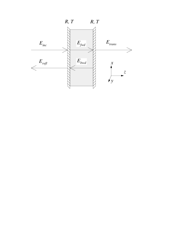
FIG. 3.: Fields and coordinate system in the Fabry-Perot cavity. The applied field $E_{inc}$ arises from a laser beam incident from the left. An atomic vapor excited to the red side of resonance by the incident light fills the space (the gray area) between the two mirrors. The presence of these atoms leads to a self-defocussing Kerr nonlinearity (corresponding to repulsive photon-photon interactions) inside the cavity.

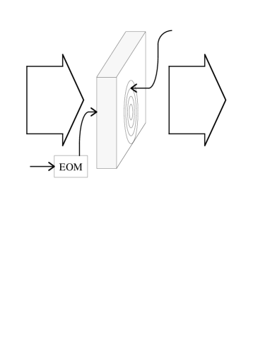
FIG. 4.: Schematic of an experiment to observe the sound-like waves in a photon fluid which fills a nonlinear Fabry-Perot resonator. The nonlinear medium (denoted by the gray area) is an alkali atomic vapor excited by a broad laser beam (denoted by the broad incoming arrow) tuned to the red side of resonance. The goal is the verify the Bogoliubov dispersion relation, Eq. (36) or (46). An electro-optic modulator (EOM) modulates the intensity of light at a radio frequency in the MHz range, which is then injected by means of an optical fiber tip at a single point on the entrance face of the Fabry-Perot resonator. The wavelength of the resulting sound-like waves can be measured by scanning in the transverse direction the tip of another optical fiber across the output face of the Fabry-Perot, and by measuring the phase of the modulated pick-up signal relative to that of the EOM modulation signal.

REFERENCES

- [1] M. H. Anderson, J. R. Ensher, M. R. Matthews, C. E .Wiemann, and E. A. Cornell, Science 269, 198 (1995).
- [2] C. C. Bradley, C. A. Sackett, J. J. Tollett, and R. G. Hulet, Phys. Rev. Lett. 75, 1687 (1995).
- [3] K. B. Davis, M.-O. Mewes, M. R. Andrews, N. J. van Druten, D. S. Durfee, D. M. Kurn, and W. Ketterle, Phys. Rev. Lett. 75, 3969 (1995).
- [4] For a review of recent work on dilute-gas Bose condensates, see A. S. Parkins and D. F. Walls, Physics Reports 303, 1 (1998); see also A. Griffin, LANL preprint cond-mat/9901123.
- [5] N. Bogoliubov, J. Phys. (U.S.S.R.) 11, 23 (1947).
- [6] D. Pines, The Many-Body Problem (Benjamin, New York, 1961).
- [7] M. W. Mitchell (private communication).
- [8] I. H. Deutsch and J. C. Garrison, Phys. Rev. A 43, 2498 (1991).
- [9] Since we have assumed a zero-temperature Bose gas, following Bogoliubov we start this calculation with the ground state of the system in the macroscopically occupied zero-momentum Fock or number state . However, it is also possible to derive the same Bogoliubov dispersion relation starting from a system in a coherent state , where . We thank Prof. David Thouless for sharing with us his unpublished notes concerning this last point.
- [10] R. E. Slusher et al., J. Opt. Soc. Am. B 4, 1453 (1987).
- [11] N. M. Hugenholtz and D. Pines, Phys. Rev. 116, 489 (1959); G. W. Goble and D. H. Kobe, Phys. Rev. A 10, 851 (1974).
- [12] It may be asked how this photon gas problem in two dimensions is different from the Planck blackbody problem in three dimensions. The first part of the answer is that the Fabry-Perot resonator makes the problem effectively two-dimensional, since the resonator is excited by a nearly monochromatic laser beam with a narrow linewidth, which selects out only a single longitudinal mode of the Fabry-Perot to be excited. Thus the degree of freedom for the photons inside the resonator is eliminated from the problem. The second part of the answer is that in contrast to the Planck problem, where the chemical potential of the photon vanishes, here there is a nonvanishing chemical potential, Eq. (25), of the photon in the photon fluid, which arises from the repulsive pairwise interactions between photons in the Bose condensate inside the Fabry-Perot resonator. For the same reasons, a two-dimensional phase transition of the Kosterlitz-Thouless type should be possible in the photon fluid.
- [13] L. A. Lugiato and R. Lefever, Phys. Rev. A 58, 2209 (1987).
-
[14]
The limit must be taken carefully. Equation
(42) assumes that the phase of the driving
field has no influence on the phase of the
internal cavity field, as . We conjecture that
this is justified when the phase of the driving laser field fluctuates
by large amounts rapidly over the time scale set by the cavity
ring-down time , as is the case when the laser linewidth
is larger than . Conversely, if we drive the cavity with a
monochromatic laser beam in a coherent state whose phase remains
constant over this time scale, the assumption leading to
Eq. (42) is invalid, and we have shown that the
dispersion relation, Eq. (46), is modified to become
when . The frequency gap which appears near becomes arbitrarily small as and we recover Eq. (46). We thank Prof. Juan Perez Torres for pointing the modified dispersion relation out to us.(49) - [15] The classical dispersion relation, Eq. (46), is also identical to the one that was derived in an early paper on stimulated light-by-light scattering (R. Y. Chiao, P. L. Kelley, and E. Garmire, Phys. Rev. Lett. 17, 1158 (1966)), apart from a sign change for the Kerr nonlinear coefficient from the self-focusing to the self-defocusing sign. The transverse spatial modulational instability of a paraxial travelling-wave configuration in a nonlinear cell, which was predicted in this paper for the self-focusing sign, upon reversal of the sign to the self-defocusing sign, turns into a kind of transverse spatial modulational stability, whose dispersion relation is identical in form to the Bogoliubov one. (This early paper should be consulted if one wants to generalize this dispersion relation to the case of a non-instantaneous response of the Kerr nonlinearity due to a finite relaxation time of the medium.) However, there is a fundamental difference between the case of light inside a nonlinear cavity and the case of light in a paraxial travelling-wave configuration inside a nonlinear cell. In a nonlinear cavity, the field envelope evolves in time , and genuine dynamics occurs inside the cavity. Hence genuine sound waves result in the limit from the classical nonlinear optical dispersion relation, Eq. (46), which would require second quantization, since we know that phonons indeed exist inside the cavity as a result of the quantum dispersion relation, Eq. (36). However, in a paraxial travelling-wave configuration, the field envelope evolves in the spatial variable , and not in the time variable . Hence the “sound waves” inside this cell are frozen, nonpropagating spatial patterns.
- [16] I. H. Deutsch, R. Y. Chiao, J. C. Garrison, Phys. Rev. Lett. 69, 3627 (1992).
- [17] R. Y. Chiao, I. H. Deutsch, J. C. Garrison, and E. W. Wright, in Frontiers in Nonlinear Optics: the Serge Akhmanov Memorial Volume, H. Walther, N. Koroteev, and M. O. Scully, eds., Institute of Physics Publishing, Bristol and Philadelphia, 1993, p. 151-182.
- [18] L. D. Landau and E. M. Lifshitz, Statistical Physics (Pergamon, London, 1958), p. 202.
- [19] Y. Pomeau and S. Rica, Comptes Rendus de l’Académie des Sciences (Paris) 317, 1287 (1993).