Complementarity and the uncertainty relations

Abstract

We formulate a general complementarity relation starting from any Hermitian operator with discrete non-degenerate eigenvalues. We then elucidate the relationship between quantum complementarity and the Heisenberg-Robertson’s uncertainty relation. We show that they are intimately connected. Finally we exemplify the general theory with some specific suggested experiments.

PACS numbers: 03.65.Bz

I Introduction

A fundamental notion of quantum mechanics is complementarity which expresses the fact that any quantum system has at least two properties that cannot simultaneously be known. One of these complementary property pairs, and perhaps the historically most important, is the wave-particle duality. A quantum system has both particle-like and wave-like properties. However, observation of one property precludes the observation of the other. Recently several quantitative expressions of this specific duality were derived [1, 2, 3, 4, 5, 6, 7, 8, 9, 10, 11], Some of these expressions have been experimentally confirmed [12, 13]. In this paper we will follow Englert’s [10] definitions most closely. In general, inequalities quantifying the wave-particle duality are posed in the context of interferometry. In any single particle interferometer it is meaningful both to ask which of the interferometer paths the particle took, and to record the visibility of a large number of identically prepared systems. In this paper we shall discuss the notions of which path and visibility in a general framework as to encompass any system defined in a two-dimensional Hilbert-space.

Let us begin by establishing some notation. Assume that we would like to estimate which of two paths, call them $+$ and $-$, a particle took. The only information we have are known probabilities $w_{+}$ and $w_{-}=1-w_{+}$ for the two events. The Maximum Likelihood (ML) estimation strategy (which is one of many possible strategies) dictates that we should, for each and every event, guess that the particle took the most likely path. The strategy will maximize the likelihood $L$ of guessing correctly. The likelihood will be $L={\rm Max}\{w_{+},w_{-}\}$, and from this relation it is evident that $1/2\leq L\leq 1$. The likelihood can be renormalized to yield the predictability $P$ [10], given by

$$P=2L-1.$$ (1)

It is clear that $0\leq P\leq 1$, where $P=0$ corresponds to a random guess of which path the particle took, and $P=1$ corresponds to absolute certainty about the path. Take note that $P$ corresponds to the likelihood of the correct estimated outcome. If one were to estimate the path of an ensemble of identically prepared particles according to the ML strategy one should guess identically the same path for each system. That is, every estimate would be identical so that the estimated path would have no variance. If, on the other hand, one made a factual measurement of the path, one would get a random outcome characterized only by the probabilities $w_{+}$ and $w_{-}$.

One could also measure the visibility when the two path probability amplitudes interfere. The visibility $V$, too, is a statistical measure which requires an ensemble of identically prepared systems to estimate. The classical definition of $V$ is

$$V={I_{max}-I_{min}\over I_{max}+I_{min}},$$ (2)

where $I_{max}$ and $I_{min}$ are the intensities of the interference fringe maxima and minima. For a single particle we can only talk about the probability $p$ of the particle falling on a specific location on a screen, or exiting one of two interferometer ports. (Do not confuse this probability $p$ with the predictability $P$.) The probability $p$ will vary essentially sinusoidally with position on the screen, or with the interferometer arm-length difference. In this case the natural definition of $V$ is

$$V={p_{max}-p_{min}\over p_{max}+p_{min}},$$ (3)

It has been shown [10] that $P$ and $V$ for a single particle, satisfies the following inequality:

$$P^{2}+V^{2}\leq 1,$$ (4)

where the upper bound is saturated for any pure state. A relevant question to ask is how this inequality is related to the uncertainty principle, which is also a quantitative inequality manifesting complementarity. Furthermore one can ask what observables, if any, $P$ and $V$ correspond to? We shall attempt to clarify these issues in this paper. We shall also show that a relation of the same form as (4) can be derived for any Hermitian operator by constructing a complementary (and therefore non-commuting) Hermitian operator. Finally we shall see that there is a substantial difference between the non-simultaneous and the simultaneous Heisenberg-Robertson uncertainty relations.

II Generalized complementarity

Let us consider the states $|A_{+}\rangle$ and $|A_{-}\rangle$, which are eigenstates of the Hermitian operator $\hat{A}$ with eigenvalues $A_{+}\neq A_{-}$, respectively. Therefore, $\langle A_{+}|A_{-}\rangle=0$. In the following we shall assume that the two-dimensional Hilbert-space spanned by these two orthonormal states is sufficient to describe the system. It is permissible that the operator $\hat{A}$ has additional eigenstates, but to analyze the complementarity relation we shall only consider transitions between, and hence superpositions of, two of the eigenstates. Below, for the sake of clarity, we shall refer to the system mode, which is the physical entity one can make measurements on, and the system state, which is the quantum-mechanical state of the mode, i.e. a result of a measurement. It is rather straightforward to extend the relation (4) to the case where a larger Hilbert-space is needed [11], but we will refrain from attempting such a generalization since two states are sufficient to elucidate the answers to the questions posed above. We shall furthermore assume that our system is prepared in a general state with the associated density operator

$$\hat{\rho}=\left[\matrix{w_{+}&\rho_{12}e^{-i\theta}\cr\rho_{12}e^{i\theta}&w_{-}}\right],$$ (5)

where $w_{+}$, $w_{-}=1-w_{+}$, $\rho_{12}\leq\sqrt{w_{+}w_{-}}$ and $\theta$ can be assumed to be real positive numbers without any loss of generality, and where the density operator is expressed in matrix form in the $|A_{+}\rangle$ and $|A_{-}\rangle$ basis. We can identify the parameter $w_{+}$ as the a priori probability of finding the system in the state $|A_{+}\rangle$, and similarly for $w_{-}$.

If we use the maximum likelihood strategy to predict the outcome of a measurement of $\hat{A}$, then we will succeed with the likelihood $L={\rm Max}\{w_{+},w_{-}\}=(w_{+}+w_{-}+|w_{+}-w_{-}|)/2=(1+|w_{+}-w_{-}|)/2$, where ${\rm Max}\{w_{+},w_{-}\}$ denotes the maximum of the two probabilities $w_{+}$ and $w_{-}$. From this equation, and (1) follows that

$$P=|w_{+}-w_{-}|=\sqrt{(1-2w_{-})^{2}}=\sqrt{1-4w_{+}w_{-}}.$$ (6)

Note that this quantity is based only on the probabilities $w_{+}$ and $w_{-}$ which characterize the preparation of the state $\hat{\rho}$.

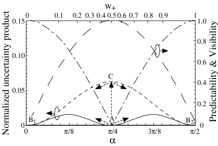
FIG. 1.: The normalized dimensionless minimum uncertainty product of the operators $\hat{A}$ and $\hat{B}$ as a function of $w_{+}=\sin^{2}(\alpha)$. The dashed line represents the uncertainty product of the second class of intelligent states. The uncertainty product of the initial state for operators $\hat{A}$ and $\hat{B}$ is bounded from below by the solid line and from above by the dashed line. The dot-dashed line represents the predictability of the state and the long dashed line the visibility of a pure state.

Next consider the two unitary operators

$$\hat{U}_{PS}=\left[\matrix{1&0\cr 0&\exp(i\phi)}\right],$$ (7)

and

$$\hat{U}_{BS}=\left[\matrix{\cos(\xi)&i\sin(\xi)\cr i\sin(\xi)&\cos(\xi)}\right],$$ (8)

which both are expressed in matrix form in the $|A_{+}\rangle$ and $|A_{-}\rangle$ basis. The two unitary transformations correspond to a generalized phase-shift (of state $|A_{-}\rangle$) and a generalized “beamsplitter”, respectively. The density matrix of the unitarily transformed state is $\hat{\rho}^{\prime}=\hat{U}_{BS}\hat{U}_{PS}\hat{\rho}\hat{U}_{PS}^{\dagger}\hat{U}_{BS}^{\dagger}$. The probability of obtaining the outcome $A_{+}$ from $\hat{\rho}^{\prime}$ if $\hat{A}$ is measured is $\langle A_{+}|\hat{\rho}^{\prime}|A_{+}\rangle$. We denote the maximum and the minimum of this probability, as a function of $\phi$ and $\xi$, $p_{max}$ and $p_{min}$. One finds that the global maxima and minima are found for $\xi=\pi/4+n\pi/2$, where $n$ is an arbitrary integer. This choice of $\xi$ corresponds to a generalized beamsplitter with a 50 % transmittivity. We use the global maxima and minima to define the visibility according to (3). It is straightforward to show that from the obtained expression follows that

$$V=2|\langle A_{+}|\hat{\rho}|A_{-}\rangle|=2\rho_{12}.$$ (9)

From this expression, and (6) follows that

$$P^{2}+V^{2}=w_{+}^{2}-2w_{+}w_{-}+w_{-}^{2}+4\rho_{12}^{2}\leq 1,$$ (10)

since $w_{+}+w_{-}=1$ and $0\leq\rho_{12}\leq\sqrt{w_{+}w_{-}}$. This re-derivation of relation (4) demonstrates that every two-state quantum system obeys a complementary relation even before any attempt has been made to simultaneously measure both $\hat{A}$ and the quantity complementary to $\hat{A}$. In Fig. 1 the generalized distinguishability and visibility are plotted dash-dotted and long dashed, respectively, as a function of $w_{+}$, parameterized by $\sin^{2}\alpha=w_{+}$.

It is obvious that $P$ in some way corresponds to a measurement of $\hat{A}$. What is the operator corresponding to the quantity represented by the visibility? To answer this question let us construct the two orthonormal states

$$|B_{+}\rangle\equiv(|A_{+}\rangle+e^{i\varrho}|A_{-}\rangle)/\sqrt{2}$$ (11)

and

$$|B_{-}\rangle\equiv(|A_{+}\rangle-e^{i\varrho}|A_{-}\rangle)/\sqrt{2}.$$ (12)

These states, in turn, can be used to construct a complementary Hermitian operator to $\hat{A}$ which is

$$\hat{B}=B_{+}|B_{+}\rangle\langle B_{+}|+B_{-}|B_{-}\rangle\langle B_{-}|,$$ (13)

where $B_{+}\neq B_{-}$ are real numbers. We have denoted this operator the complementary operator to $\hat{A}$ since the eigenstates of $\hat{B}$ are equally weighted superpositions of the eigenstates of $\hat{A}$. Hence, if we prepare a state so that the outcome of a measurement corresponding to $\hat{A}$ can be predicted with certainty, then nothing can be predicted about the measurement outcome corresponding to $\hat{B}$, and vice versa. Since the eigenstates of $\hat{B}$ are parameterized by $\varrho$ there exists a whole set of complementary operators to $\hat{A}$. We note that irrespective of $\varrho$, the states $|B_{+}\rangle$ and $|B_{-}\rangle$ are the Hadamard transformations of the $|A_{+}\rangle$ and $|A_{-}\rangle$ states. This is no coincidence since the fact that $\hat{B}$ is the complementary operator to $\hat{A}$ makes the two corresponding bases optimal for quantum cryptography. This brings in light the intimate link [14] between the complementarity relations, quantum information and quantum cryptography.

It should be noted that the observable $\hat{A}$ plays no particular role vis-a-vis the observable $\hat{B}$ in the expression (10). Assume that the state $\hat{\rho}$ remains invariant, but that $\hat{A}$ and $\hat{B}$ are interchanged so that the maximum likelihood estimation and the generalized visibility measurement pertains to the outcome of a measurement of $\hat{B}$, and that new unitary transformations are defined that have identically the same form as (7) and (8) if expressed in the $|B_{+}\rangle$ and $|B_{-}\rangle$ basis. Then we find that

$$P_{B}=2\rho_{12}|\cos(\theta-\varrho)|$$ (14)

(where we have labeled this predictability with an index $B$ not to confuse it with the predictability of estimating $\hat{A}$) and that the new “visibility” is given by

$$V_{B}=\sqrt{w_{+}^{2}+w_{-}^{2}-2w_{+}w_{-}+4\rho_{12}^{2}\sin^{2}(\theta-\varrho)}.$$ (15)

Hence, although the likelihood of estimating $\hat{B}$ correctly in general is different from the likelihood of estimating $\hat{A}$, relation (10) still holds. We observe that it is always possible to find an operator $\hat{B}$ for which the predictability between the measurement outcomes is zero. This represents the quantum erasure measurement operator [4, 7, 8, 11, 12, 15, 16]. However, the sum $P^{2}+V^{2}$ remains invariant and depends only on the state, not on the choice of complementary operators by which one estimates and measures $P$ and $V$.

To explore the symmetry between the pairs $\hat{A}$ and $\hat{B}$, we can see from (9) and (14) that the predictability $P_{B}$ of a measurement of the proper $\hat{B}$ operator is

$$P_{B}=2\rho_{12}=V$$ (16)

By the “proper $\hat{B}$ operator” we mean the complementary operator to $\hat{A}$ that, for the state $\hat{\rho}$, optimizes the visibility (or minimizes the variance of $\hat{B}$, see below). Therefore the operator is defined with $\varrho=\theta$. Note that the word proper hence is in reference to the measured state. In the same manner we see from (6) and (15) that for the proper $\hat{B}$ operator

$$V_{B}=|w_{+}-w_{-}|=P.$$ (17)

III The Heisenberg-Robertson uncertainty relation

The commutator between $\hat{A}$ and $\hat{B}$ follows from the definition of the operators and can be expressed:

$$[\hat{A},\hat{B}]=(A_{+}-A_{-})(B_{+}-B_{-})(|A_{+}\rangle\langle A_{-}|-|A_{-}\rangle\langle A_{+}|).$$ (18)

We see that the operators $\hat{A}$ and $\hat{B}$ are non-commuting, non-canonical operators. Since the operators are non-canonical they will be subject to a generalized uncertainty inequality [17, 18, 19, 20, 21]. The uncertainty inequality reads

$$\langle(\Delta\hat{A})^{2}\rangle\langle(\Delta\hat{B})^{2}\rangle\geq{1\over 4}\left(\langle\hat{C}\rangle^{2}+\langle\hat{F}\rangle^{2}\right),$$ (19)

where the $\hat{C}$ is directly proportional to the commutator and is defined as

$$\hat{C}=-i[\hat{A},\hat{B}],$$ (20)

and $\langle\hat{F}\rangle$ is the correlation between the observables and is defined

$$\langle\hat{F}\rangle=\langle\hat{A}\hat{B}+\hat{B}\hat{A}\rangle-2\langle\hat{A}\rangle\langle\hat{B}\rangle.$$ (21)

The expectation value and the variance of the state (5) can be computed to be

$$\langle\hat{A}\rangle=A_{+}w_{+}+A_{-}w_{-},$$ (22)

and

$$\langle(\Delta\hat{A})^{2}\rangle=(A_{+}-A_{-})^{2}w_{+}w_{-}.$$ (23)

Using (6) we can write

$${\langle(\Delta\hat{A})^{2}\rangle\over(A_{+}-A_{-})^{2}}={1-P^{2}\over 4}.$$ (24)

This equation shows the direct link between a measurement of the operator $\hat{A}$ and the predictability $P$. If e.g. $P$ is unity, then the variance of $\hat{A}$ is zero.

To show that a similar relation holds between $\hat{B}$ and $V$ we compute:

$$\langle\hat{B}\rangle = {B_{+}\over 2}\,[1+2\rho_{12}\cos(\theta-\varrho)]$$ (26)

$$+{B_{-}\over 2}\,[1-2\rho_{12}\cos(\theta-\varrho)],$$

and

$$\langle(\Delta\hat{B})^{2}\rangle=(B_{+}-B_{-})^{2}{1-4\rho_{12}^{2}\cos^{2}(\theta-\varrho)\over 4}.$$ (27)

The variance of $\hat{B}$ is minimized for the proper operator $\hat{B}$. We note that for the proper complementary operator, the normalized and dimensionless variance is given by

$${\langle(\Delta\hat{B})^{2}\rangle\over(B_{+}-B_{-})^{2}}={1-4\rho_{12}^{2}\over 4}={1-V^{2}\over 4}.$$ (28)

The visibility is thus directly linked to the variance, or uncertainty, of the proper complementary operator to $\hat{A}$. As a final result we note that the normalized uncertainty product can be written

$${\langle(\Delta\hat{A})^{2}\rangle\langle(\Delta\hat{B})^{2}\rangle\over(A_{+}-A_{-})^{2}(B_{+}-B_{-})^{2}} \geq w_{+}w_{-}{1-4\rho_{12}^{2}\over 4}=$$ (30)

$${(1-P^{2})(1-V^{2})\over 16}.$$

Hence, there is a direct link between the complementarity relation (4) and the minimum uncertainty product. This is one of the main conclusions of this paper. The result is true regardless if the state in question is pure or mixed. However, for a pure state the right hand side of (30) can be further simplified to read

$${\langle(\Delta\hat{A})^{2}\rangle\langle(\Delta\hat{B})^{2}\rangle\over(A_{+}-A_{-})^{2}(B_{+}-B_{-})^{2}}\geq{V^{2}P^{2}\over 16}.$$ (31)

In Fig. 1 the normalized minimum uncertainty product (solid line) is plotted versus the probability $w_{+}$. The dashed line represents the maximum uncertainty product.

The Robertson intelligent states $|\psi_{IS}\rangle$ are given by the eigenstate solution of the equation [21]

$$(\hat{A}+i\lambda\hat{B})|\psi_{IS}\rangle=(\langle\hat{A}\rangle+i\lambda\langle\hat{B}\rangle)|\psi_{IS}\rangle.$$ (32)

The complex parameter $\lambda$ satisfies $|\lambda|^{2}=\langle(\Delta\hat{A})^{2}\rangle/\langle(\Delta\hat{B})^{2}\rangle$. We will here give the solutions for the cases where $\lambda$ is either real or imaginary [20]. For imaginary $\lambda$ we find

$$|\psi_{IS1}\rangle=\sqrt{w_{+}}|A_{+}\rangle\pm e^{i\varrho}\sqrt{w_{-}}|A_{-}\rangle.$$ (33)

As $|\lambda|$ increases from zero towards infinity the two solutions evolve from $w_{+}=1/2$ towards $w_{+}\rightarrow 0$ and $w_{+}\rightarrow 1$, respectively (from point A to points B₁ and B₂ in Fig. 1). The minimum uncertainty states (which are the intelligent states with the minimum uncertainty) belong to this class of intelligent states with $w_{+}=0$, 1/2, and 1, respectively. As expected these are the eigenstates of $\hat{A}$ and $\hat{B}$. The intelligent states with $\lambda$ real are given by

$$|\psi_{IS2}\rangle={1\over\sqrt{2}}(|A_{+}\rangle\pm e^{i(\varrho\pm\beta)}|A_{-}\rangle).$$ (34)

When $|\lambda|$ goes from 0 towards 1, $\beta$ goes from 0 to $\pi/2$ (and the uncertainty product goes along the dotted line from point A to point C in Fig. 1). When subsequently $1\leq|\lambda|\rightarrow\infty$, the second class of intelligent states becomes

$$|\psi_{IS2}\rangle=\sqrt{w_{+}}|A_{+}\rangle\pm ie^{i\varrho}\sqrt{w_{-}}|A_{-}\rangle,$$ (35)

where $w_{+}$ evolves from 1/2 towards 0 and from 1/2 towards 1, for the respective states. (The uncertainty product goes along the dashed line from point C to points B₁ and B₂.) The two sets of intelligent states considered above are found to be the states with extreme uncertainty products.

IV Complementary two-state operators

In the preceding section we saw that there are infinitely many complementary operators to $\hat{A}$. However, for any choice of $\varrho$ there are only two sets of three mutually complementary operators. If we explicitly write out the operator $\hat{B}$ as a function of $\varrho$, v.i.z. $\hat{B}(\varrho)$, then the two sets are $\hat{A}$, $\hat{B}(\varrho)$, $\hat{B}(\varrho+\pi/2)$ and $\hat{A}$, $\hat{B}(\varrho)$, $\hat{B}(\varrho-\pi/2)$. To clarify the meaning of this statement we note that the operator pair $\hat{A}$ and $\hat{B}(\varrho)$, the pair $\hat{A}$ and $\hat{B}(\varrho+\pi/2)$ as well as the pair $\hat{B}(\varrho)$ and $\hat{B}(\varrho+\pi/2)$ are all complementary. This is the meaning of the term “a set of mutually complementary operators”.

To identify such an abstract set of operators with one (of many) specific observables we can e.g. assume that $\hat{A}$ corresponds to the spin $z$ operator $\hat{\sigma}_{z}$ of a spin 1/2 particle, with eigenvalues $\pm\hbar/2$. If we furthermore assume that the eigenvalues of the operators $\hat{B}(\varrho)$ and $\hat{B}(\varrho\pm\pi/2)$ are $B_{1}=-B_{2}=\hbar/2$, we readily recognize the other two complementary operators as the spin $\hat{\sigma}_{u}$ and $\hat{\sigma}_{v}$ operators, where $u,v,z$ denotes a right-handed (left-handed) orthogonal Euclidian vector set for the choice $\varrho+\pi/2$ ($\varrho-\pi/2$). With this choice the commutation relation (18) reduces to the familiar spin operator commutator $[\hat{\sigma}_{i},\hat{\sigma}_{j}]=i\hbar\epsilon_{ijk}\hat{\sigma}_{k}$ with $i,j,k\rightarrow u,v,z$, in this case.

Note, however, that orthogonal spin operators is only one realization of a mutually complementary set. One can construct infinitely many such triplets of operators for every two-state system. In [22, 23] such a triplet set was constructed starting from two orthogonally polarized single photon states. The three pairs of eigenstates were subsequently used as bases in a six-state quantum cryptography protocol. We think that a generalization of this idea of mutually complementary operators in Hilbert-spaces of higher dimension have an obvious application for the construction of eavesdropping-safe quantum cryptographic protocols.

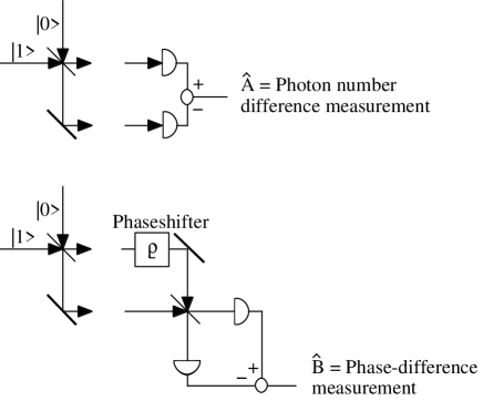
FIG. 2.: An example of complementary operators. The single photon two-mode state prepared at left can be measured either by a number-difference operator (top) or by a phase-difference measurement (bottom). By adjusting the phase shift $\varrho$ any operator $\hat{B}(\varrho)$ can be implemented.

As a second example of complementary operator pairs we consider a single particle in a well defined spatio-temporal mode, impinging on a symmetric Mach-Zehnder interferometer. The particle can take either of the two paths. The corresponding states can be written $|1\rangle\otimes|0\rangle$ and $|0\rangle\otimes|1\rangle$. Defining $\hat{A}$ to be the two-mode particle number-difference operator $(\hat{n}_{1}-\hat{n}_{2})/2$ with the eigenvectors above and with eigenvalues $\pm 1/2$, we find that the operator $\hat{B}$ corresponds to the two-mode phase-difference operator (in the first particle manifold) defined by Luis and Sánchez-Soto [24, 25, 26]:

$$\hat{\phi}_{12}=\theta|\phi_{1}\rangle\langle\phi_{1}|+(\theta+\pi)|\phi_{2}\rangle\langle\phi_{2}|,$$ (36)

where $|\phi_{1}\rangle=(|1\rangle\otimes|0\rangle+e^{i\varrho}|0\rangle\otimes|1\rangle)/\sqrt{2}$ and $|\phi_{2}\rangle=(|1\rangle\otimes|0\rangle-e^{i\varrho}|0\rangle\otimes|1\rangle)/\sqrt{2}$, and the corresponding eigenvalues are $\theta$ and $\theta+\pi$. Fig. 2 provides a schematic illustration of the implementation of the state preparation (left) and the operator set (right).

Note that the proper operators in this case, where the eigenstates are discrete, do not correspond to position and momentum operators, as textbook discussions of this specific interferometric duality experiment often indicate. This has already been noted and discussed by de Muynck [27]. In the same vein Luis and Sánchez-Soto have used the phase-difference operator to analyze the mechanism which enforces complementarity, and specifically loss of fringe visibility with increasing distinguishability [26].

Identifying the operator $\hat{A}$ with any Hermitian operator (for which it makes sense to have a restricted two-state Hilbert-space) it is always possible to write down a complementarity relation for $\hat{A}$. Since the form of the complementary operator $\hat{B}$ to $\hat{A}$ is known, and it has a simple form, it is often possible to identify this operator with some known observable. Since complementarity follows directly from the superposition principle, and therefore permeates all of quantum mechanics, the term welcher weg experiment which is intimately tied to complementarity should perhaps be replaced by the term welcher zustand experiment.

V Complementarity and uncertainty relations for simultaneous measurements

So far we have discussed the standard Heisenberg-Robertson uncertainty relation which makes a statement about the preparation of a state. E.g. the variance of $\hat{A}$ computed in (23) is the variance associated with a sharp measurement of $\hat{A}$ on an ensemble of systems all prepared in the state $\hat{\rho}$. The measurement will either destroy the state or collapse the state into an eigenstate of $\hat{A}$ so the sharp measurement will preclude any meaningful subsequent measurement of $\hat{B}$. However, it is also interesting to see what the uncertainty product becomes if one tries to simultaneously measure $\hat{A}$ and $\hat{B}$. By “simultaneous” we mean that we make (necessarily unsharp) measurements of both $\hat{A}$ and $\hat{B}$ on each individual system mode in the ensemble. In order to do so we need to entangle the system with an auxiliary meter mode, associated with an arbitrarily large Hilbert-space ${\cal H}_{m}$, see Fig. 3. If the entanglement between the system and meter modes is perfect (to be quantified below), then a sharp measurement of the state of the meter mode will collapse the system mode into an eigenstate of e.g. $\hat{A}$. This is the principle of a quantum non-demolition measurement. However, in order to subsequently be able to say something about $\hat{B}$ of the initial system state from the same copy of the quantum state, the entanglement cannot be perfect, and to be able to say something about $\hat{A}$ it cannot be zero. Therefore both the $\hat{A}$ and the $\hat{B}$ measurements need to be unsharp, that is, associated with additional statistical uncertainties than what follows from the preparation of the state. This is well known for simultaneous measurements [27, 28, 29, 30, 31, 32].

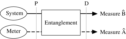
FIG. 3.: A schematic representation of a simultaneous measurement of $\hat{A}$ and $\hat{B}$ on a single system. The planes P and D denote the spatial points where it is appropriate to measure $P$ or $V$, and $D$ or $V_{e}$, respectively. If an unsharp measurement is performed $D$ and $V_{e}$ can be measured at plane D.

In the following we will only treat the case where the composite system is pure as this will set the lower limit to our ability to simultaneous measure or predict the values of the observables $\hat{A}$ and $\hat{B}$. We shall assume that the entanglement is accomplished through some unitary operation which does not change the probabilities $w_{+}$ and $w_{-}$. (The more general case is discussed in [11]). Such an entanglement should perhaps be called quantum non-demolition measurement type entanglement (where the word measurement refers to $\hat{A}$), since a perfect entanglement of this type will allow one to make a sharp QND measurement of $\hat{A}$. This is not the most general form of entanglement, but it is the type of entanglement needed for our purposes, so a sufficiently general pure state of the entangled system can be written

$$|\psi_{e}\rangle = \sqrt{w_{+}}|A_{+}\rangle\otimes|M_{+}\rangle+e^{i\theta}\sqrt{w_{-}}|A_{-}\rangle\otimes|M_{-}\rangle$$ (37)

$$\equiv \sqrt{w_{+}}|A_{+}\rangle\otimes|M_{+}\rangle$$ (39)

$$+e^{i\theta}\sqrt{w_{-}}|A_{-}\rangle\otimes(c|M_{+}\rangle+\sqrt{1-c^{2}}|M_{\perp}\rangle),$$

where $c$ is real and positive and defined by $|\langle M_{-}|M_{+}\rangle|=c$, and $\langle M_{+}|M_{\perp}\rangle=0$. We see that since $\hat{A}$ has a binary measurement outcome, we need only consider the reduced 2-dimensional meter mode Hilbert-space ${\cal H}_{r}$ spanned by $|M_{+}\rangle$ and $|M_{\perp}\rangle$. The density operator associated with $|\psi_{e}\rangle$ will be denoted $\hat{\rho}_{e}$. With the help of the parameter $c$, which is a measure of the entanglement between the modes, the distinguishability $D$ based on an optimal measurement of the meter mode, can be expressed

$$D\equiv||\langle A_{+}|\hat{\rho}_{e}|A_{+}\rangle-\langle A_{-}|\hat{\rho}_{e}|A_{-}\rangle||_{1}=\sqrt{1-4c^{2}w_{+}w_{-}}.$$ (40)

(The notation $||\hat{O}||_{1}\equiv{\rm Tr}\{\sqrt{\hat{O}^{\dagger}\hat{O}}\}$ denotes the trace-class norm of the operator $\hat{O}$.) The distinguishability $D$ has the same connection to the likelihood of guessing correctly about the outcome of a sharp $\hat{A}$ measurement, that is $D=2L-1$. However, $D$ is associated with a factual measurement and not simply by an estimate based on a priori knowledge. It may be noted that $P\leq D$ always holds [10, 11] provided the QND-type of entanglement is used.

The visibility $V_{e}$ of the entangled system is given by

$$V_{e}=2|\langle A_{-}|{\rm Tr}_{r}\{\hat{\rho}_{e}\}|A_{+}\rangle|=2c\sqrt{w_{+}w_{-}},$$ (41)

where the partial trace is taken over ${\cal H}_{r}$. Since the state $|\psi_{e}\rangle$ is pure, the relation

$$D^{2}+V_{e}^{2}=1$$ (42)

holds [10].

A measurement of the meter mode will allow us to deduce more or less about the initial state of the system (5). If e.g. $c=0$, then the wavefunction (39) represents a maximally entangled state and a measurement of the meter mode, using $|M_{+}\rangle$ and $|M_{\perp}\rangle$ as projection bases, will yield a perfect correlation with a subsequent $\hat{A}$ measurement of the system mode. However, as noted above, such a measurement of the meter mode will preclude any meaningful information to be reaped about the complementary observable $\hat{B}$. Therefore, we will in the following discuss how to perform an optimal simultaneous measurement of $\hat{A}$ and $\hat{B}$. With simultaneous we understand a measurement where we try to obtain some information of both $\hat{A}$ and $\hat{B}$ from a single copy of a pure state (5) which after an entangling interaction is transformed to (39).

To find the minimum uncertainty product of a simultaneous measurement of $\hat{A}$ and $\hat{B}$ we have assumed that the $\hat{A}$ information will be obtained by making a sharp measurement of the meter mode, and the $\hat{B}$ information will be obtained by making a subsequent sharp measurement on the system mode. (We note that one could also have chosen to do the opposite. However, if we do so, the system and meter modes should be entangled in a different manner than what has been assumed above. Still, if we choose the inverse measurement procedure and do it optimally, the final result, quantified by a simultaneous uncertainty product, remains identical to the result below.) Let us start with the $\hat{B}$ measurement. The two pertinent projectors are $|B_{+}\rangle\langle B_{+}|$ and $|B_{-}\rangle\langle B_{-}|$. The associated probabilities are

$$P_{B_{\pm}}=\langle B_{\pm}|{\rm Tr}_{r}\{\hat{\rho}_{e}\}|B_{\pm}\rangle={1\over 2}\pm c\sqrt{w_{+}w_{-}}\cos(\theta-\varrho).$$ (43)

If the two outcomes are associated with the values $B_{+}^{\prime}$ and $B_{-}^{\prime}$, then the mean of the measurement, or rather estimation, of $\hat{B}$ (which we will denote $\hat{B}^{\prime}$) will yield

$$\langle\hat{B}^{\prime}\rangle={B_{+}^{\prime}+B_{-}^{\prime}\over 2}+(B_{+}^{\prime}-B_{-}^{\prime})c\sqrt{w_{+}w_{-}}\cos(\theta-\varrho).$$ (44)

We note that, without loss of generality, we can assume a gauge such that the true eigenvalues $B_{+}$ and $B_{+}$ fulfill $B_{+}=-B_{-}=B$, and hence $B_{+}^{\prime}=-B_{-}^{\prime}=B^{\prime}$. To make the estimated mean (44) equal the true mean (26) we set $B_{\pm}^{\prime}=B_{\pm}/c$. We point out that the choice is independent of the initial state of the system mode (which is characterized by $w_{+}$ and $\theta$), but depends on the degree of entanglement $c$. The assumption of a “true mean” meter is essential to what follows, and is also made by Arthurs, Kelly and Goodman in their seminal papers on simultaneous measurements [28, 29]. From the assumption follows that the variance of the estimate of $\hat{B}$ is

$$\langle(\Delta\hat{B}^{\prime})^{2}\rangle = {(B_{+}^{\prime}-B_{-}^{\prime})^{2}\over 4}\,[1-4c^{2}w_{+}w_{-}\cos^{2}(\theta-\varrho)]$$ (45)

$$= B^{2}\left({1\over c^{2}}-4w_{+}w_{-}\cos^{2}(\theta-\varrho)\right).$$ (46)

It is obvious from this expression that in order to minimize the variance of the estimate of $\hat{B}$, one should choose $\theta=\varrho$. We also see that when $c=1$, that is, when the system and meter modes are unentangled, the result reduces identically to (27). On the other hand, when $c\rightarrow 0$, the variance diverges in spite of the fact that $\hat{B}$ has a finite number of finite eigenvalues. This is a consequence of our requirement that the mean of the estimate should equal the true mean of the state.

If the (proper) choice $\theta=\varrho$ is made, then we can express the normalized variance in the visibility (41):

$${\langle(\Delta\hat{B}^{\prime})^{2}\rangle\over(B_{+}^{\prime}-B_{-}^{\prime})^{2}}={1-V_{e}^{2}\over 4}$$ (47)

It is to be expected that such a relation holds, because the visibility, as shown above, corresponds to a sharp measurement of the uncertainty of operator $\hat{B}$.

In order to best estimate the outcome of a measurement of $\hat{A}$ of the initial system state from a measurement on the meter mode, we need to find the optimal projectors. Since the entangled state (39) can be expressed in a 2 $\times$ 2 Hilbert space, we need only construct two meter mode projectors. The most general forms for the projector-states are

$$|M_{1}\rangle=\cos(\gamma)|M_{+}\rangle+e^{i\kappa}\sin(\gamma)|M_{\perp}\rangle$$ (48)

and

$$|M_{2}\rangle=-\sin(\gamma)e^{i\kappa}|M_{+}\rangle+\cos(\gamma)|M_{\perp}\rangle.$$ (49)

However, it is immediately obvious that in order to best estimate $\hat{A}$ the choice $\kappa=0$ (or $\kappa=\pi$ which is equivalent to $|M_{1}\rangle\leftrightarrow|M_{2}\rangle$) should be made since $|M_{\perp}\rangle$ is defined such that $c$ is real. Furthermore, again we shall assume that a gauge is chosen so that $A_{+}=-A_{-}=A$, and therefore the measurement values associated with the two outcomes $A_{+}^{\prime}$ and $A_{-}^{\prime}$ fulfill $A_{+}^{\prime}=-A_{-}^{\prime}=A^{\prime}$. With this choice, the expectation value of the estimate of $\hat{A}$ (which we call $\hat{A}^{\prime}$) becomes

$$\langle\hat{A}^{\prime}\rangle = A^{\prime}\{[\cos^{2}(\gamma)-\sin^{2}(\gamma)][w_{+}-w_{-}(1-2c^{2})]$$ (51)

$$+4w_{-}c\sqrt{1-c^{2}}\cos(\gamma)\sin(\gamma)\}$$

We see that in order to make the estimated mean correct, c.f. (22), and independent of the initial system state, the following two conditions must be met:

$${\cos^{2}(\gamma)-\sin^{2}(\gamma)\over 2\cos(\gamma)\sin(\gamma)}=-{\sqrt{1-c^{2}}\over c}$$ (52)

and

$$A^{\prime}={A\over\cos^{2}(\gamma)-\sin^{2}(\gamma)}={A\over\sqrt{1-c^{2}}},$$ (53)

where the second equality in (53) follows from (52). Note that both conditions are state independent. That is, $\langle\hat{A}^{\prime}\rangle=\langle\hat{A}\rangle$ irrespective of $w_{+}$ and $\theta$ if the two conditions are met. The variance of the estimate of $\hat{A}$ can then be computed to be

$$\langle(\Delta\hat{A}^{\prime})^{2}\rangle=A^{2}\left({c^{2}\over 1-c^{2}}+4w_{+}w_{-}\right).$$ (54)

We see that, as expected, the estimated variance equals the true variance for $c=0$, that is, when the system and meter modes are maximally entangled. The estimated variance diverges when $c\rightarrow 1$. This, too, is a consequence of requiring a correct estimated mean.

The normalized and dimensionless simultaneous uncertainty product is hence

$${\langle(\Delta\hat{A}^{\prime})^{2}\rangle\langle(\Delta\hat{B}^{\prime})^{2}\rangle\over 16A^{2}B^{2}}$$ (56)

$$=\left({c^{2}\over 4(1-c^{2})}+w_{+}w_{-}\right)\left({1\over 4c^{2}}-w_{+}w_{-}\right).$$

As expected, the uncertainty product is larger than (30) and depends both on the initial state and on the degree of entanglement between the system mode and the meter mode. The entanglement parameter $c$ can be used to shift the measurement uncertainty, to some extent, from one of the operators to the complementary one.

If, for each choice of $w_{+}$, we optimize the entanglement to minimize the uncertainty product, and this is the principle used in [28, 29] to derive the minimum uncertainty product for a simultaneous measurement of two canonical non-commuting operators, then the ensuing normalized minimum uncertainty product is given by:

  

$${\langle(\Delta\hat{A})^{2}\rangle\langle(\Delta\hat{B})^{2}\rangle\over 16A^{2}B^{2}}={-16w_{+}^{2}w_{-}^{2}(1-4w_{+}w_{-})^{2}+[1-12w_{+}w_{-}(1-4w_{+}w_{-})]\sqrt{w_{+}w_{-}(1-4w_{+}w_{-})}\over 16[-4w_{+}w_{-}(1-4w_{+}w_{-})+\sqrt{w_{+}w_{-}(1-4w_{+}w_{-})}]}$$ (57)

and this expression holds for

$$c=\sqrt{{-4w_{+}w_{-}+2\sqrt{w_{+}w_{-}(1-4w_{+}w_{-})}}\over 1-8w_{+}w_{-}}.$$ (58)

This is the other major result of this paper, where the physical implications of (57) rather than the (rather messy) form should be retained. Remember that this result is contingent on a priori information about the preparation of the state (i.e. to be able to make a minimum uncertainty measurement of the state, $w_{+}$ and $\theta$ must be known). The result is plotted in Fig. 4, solid line. This is the minimum uncertainty of a simultaneous measurement of the two complementary and non-canonical operators $\hat{A}$ and $\hat{B}$. The result should be compared with the standard uncertainty product (30) of a state in two-dimensional Hilbert-space.

The corresponding distinguishability and visibility are plotted as dash-dotted and long dashed lines, respectively, in Fig. 4. We have assumed that the entanglement parameter $c$ for each $w_{+}$ is chosen according to (58). By necessity the distinguishability is higher than the predictability for the entangled state while the visibility is correspondingly lower than for the initial state (c.f. Fig. 1). We also observe that due to the “noise term” in (54) there is no simple connection between the uncertainties of $\hat{A}^{\prime}$ and the distinguishability (40). Therefore one cannot find any general relation between (42) and the non-simultaneous uncertainty relation (30). This was noted already by Englert who asserted that “…the duality relation (42) is logically independent of the uncertainty relation ….” The reason is that whereas $\langle(\Delta\hat{A})^{2}\rangle$, $\langle(\Delta\hat{B})^{2}\rangle$, $P$, $V$ and $V_{e}$ all correspond to the uncertainties of factual measurements, $D$ does not. Instead it characterizes a ML estimate, which cannot be directly related to a factual measurement of the corresponding operator.

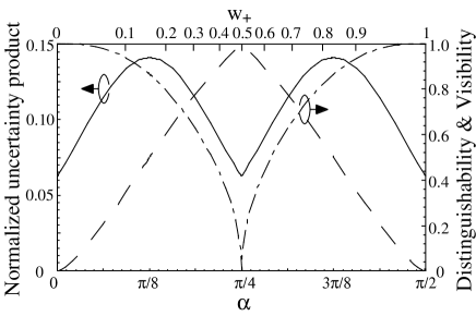
FIG. 4.: The normalized dimensionless minimum uncertainty product for a simultaneous measurement of the operators $\hat{A}$ and $\hat{B}$, solid line. The dot-dashed line represents the distinguishability and the long dashed line the visibility of the entangled state, provided that the optimum entanglement parameter $c$ is chosen for each value of $w_{+}$.

It is interesting to make a connection between (57) and (30) via (58). We have already noted that the two uncertainty relations are different since they represent physically different measurements on physically different states. However, we have striven, as far as possible, to try to design a “fair” procedure to simultaneous measure $\hat{A}$ and $\hat{B}$ of the state (5) through a measurement of the state (39). Specifically we have required that the expectation values of the corresponding measurements coincide. Using the fact that the optimum entanglement given by (58) can be expressed

$$c=\sqrt{{V(P-V)\over P^{2}-V^{2}}},$$ (59)

some somewhat tedious algebra will show that the normalized simultaneous uncertainty product can be expressed

$${\langle(\Delta\hat{A}^{\prime})^{2}\rangle\langle(\Delta\hat{B}^{\prime})^{2}\rangle\over 16A^{2}B^{2}}={(1-VP)^{2}\over 16}.$$ (60)

This rather remarkably simple result should be compared to (30) and (31). Hence, we see that our requirement of correct expectation values enforces a simultaneous uncertainty product which is uniquely dictated by the preparation of the state. This is not wholly surprising as e.g. the eigenstates of $\hat{A}$ and $\hat{B}$ could reasonably be expected to have the smallest simultaneous uncertainty product.

Appleby [32] has argued that the simultaneous uncertainty relation is less general than the Heisenberg-Robertson uncertainty relation. We agree, and this is demonstrated by our analysis. While the Heisenberg-Robertson uncertainty relation is based on sharp, non-simultaneous measurements of the two complementary operators, and therefore operationally well defined, the simultaneous uncertainty relation is based on unsharp measurements. How should these unsharp measurements be performed? More specifically, how should e.g. the meter-state projection basis (48) and (49) be chosen, and how should the outcomes of the meter-system measurement be interpreted? We have, following Arthurs and Kelly, required that the expectation value of the unsharp measurement equals the true mean. This requirement enters our analysis through (52) and (53). In Appleby’s terminology this defines a retrodictively unbiased measurement. This is, however, not the only reasonable choice. We can instead choose the meter-state projection basis to optimize the distinguishability for every value of the entanglement parameter $c$. With this choice one cannot make a state-independent retrodictively unbiased measurement. None-the-less, the choice is reasonable but will result in a different minimum uncertainty relation than the one we derived. In our eyes, if the meter projection basis is chosen to optimize the distinguishability, it is more natural to make the quantitative statement of complementarity in terms of equation (42). The conclusion is that any expression that makes a statement of a simultaneous measurement of complementary observables irrevocably must involve properties of the meter, in addition to the properties of the state.

It is noteworthy that the simultaneous uncertainty relation we derived differs from that derived by Arthurs, Kelly, and Goodman [28, 29]. They, and subsequent workers, implicitly or explicitly assumed that the pertinent operators were canonical, and in this case the uncertainty product for a simultaneous measurement is simply four times larger than the standard uncertainty product. In our case the situation is more complex. Due to the fact that $\hat{A}$ and $\hat{B}$ are non-canonical the uncertainty product of a simultaneous measurement is not simply scaled by a constant factor. Specifically, the simultaneous uncertainty product of the eigenstates to $\hat{A}$ and $\hat{B}$ is non-zero due to the “correct mean assumption”. We believe that this is a general result for any non-canonical observables.

VI Conclusions

In physics textbooks quantum complementarity is often exemplified in terms of one “particle” passing through a double-slit. The complementary observables are usually taken to be the canonical position and momentum operators, without much justification. We have shown how complementarity is a natural consequence of the superposition principle, and explored the connection between complementarity and the uncertainty relations. We have shown that for any two-state system one can always formulate a generalized complementarity relation, and that this relation typically cannot be interpreted in terms of position and momentum operators. We have also indicated that for a system with a discrete number of non-degenerate eigenstates, the corresponding operators are not canonical. Never-the-less, for a two-state system simple and rather intuitive relations hold between expressions of complementarity and uncertainty.

We have also shown that if a simultaneous measurement of complementary operators is made on a two-state system, a different uncertainty relation arises than that derived by Arthurs and Kelly. Finally, we have indicated some natural connections between complementarity and quantum information. This is to be expected since a two-state system is a natural physical manifestation of a qubit, irrespective of its particular physical implementation (spin, excitation, charge, etc.).

REFERENCES

- [1] W. K. Wootters and W. H. Zurek, Phys. Rev. D 19, 473 (1979).
- [2] D. M. Greenberger and A. Yasin, Phys. Lett. A 128, 391 (1988).
- [3] L. Mandel, Opt. Lett. 16, 1882 (1991).
- [4] M. O. Scully, B.-G. Englert, and H. Walther, Nature (London) 351, 111 (1991).
- [5] M. G. Raymer and S. Yang, J. Mod. Opt. 39, 1221 (1992).
- [6] P. G. Kwiat, A. M. Steinberg, and R. Chiao, Phys. Rev. A 45, 7729 (1992).
- [7] S. M. Tan and D.F. Walls, Phys. Rev. A 47, 4663 (1993).
- [8] P. G. Kwiat, A. M. Steinberg, and R. Chiao, Phys. Rev. A 49, 61 (1994).
- [9] G. Jaeger, A. Shimony, and L. Vaidman, Phys. Rev. A 51, 54 (1995).
- [10] B.-G. Englert, Phys. Rev. Lett. 77, 2154 (1996).
- [11] G. Björk and A. Karlsson, Phys. Rev. A 58, 3477 (1998).
- [12] T. J. Herzog, P. G. Kwiat, H. Weinfurter, and A. Zeilinger, Phys. Rev. Lett. 75, 3034 (1995).
- [13] S. Dürr, T. Nonn, and G. Rempe, Phys. Rev. Lett. 81, 5705 (1998).
- [14] C. A. Fuchs and A. Peres, Phys. Rev. A 53, 2038 (1996).
- [15] M. O. Scully and K. Drühl, Phys. Rev. A 25, 2208 (1982).
- [16] Y.-H. Kim, R. Yu, S. P. Kulik, Y. H. Shih, and M. O. Scully, Los Alamos e-print archive quant-ph/9903047.
- [17] E. Schrödinger, Proc. of the Prussian Academy of Sciences Physics-Mathematical Section, XIX, 296 (1930). An english translation can be found in Los Alamos e-print archive quant-ph/9903100.
- [18] H. P. Robertson, Phys. Rev. 35, 667A (1930); 46, 7941 (1934).
- [19] E. Merzbacher, Quantum Mechanics (Wiley, New York, 1970).
- [20] R. R. Puri, Phys. Rev. A 49, 2178 (1994).
- [21] D. A. Trifonov, J. Math. Phys. 35, 2297 (1994).
- [22] D. Bruß, Los Alamos e-print archive quant-ph/9805019.
- [23] H. Bechmann-Pasquinucci and N. Gisin, Los Alamos e-print archive quant-ph/9807041 v2.
- [24] A. Luis and L. L. Sánchez-Soto, Phys. Rev. A 48, 4702 (1993).
- [25] A. Luis and L. L. Sánchez-Soto, Phys. Rev. A 53, 495 (1996).
- [26] A. Luis and L. L. Sánchez-Soto, Phys. Rev. Lett. 81, 4031 (1998).
- [27] W. M. de Muynck, Los Alamos e-print archive quant-ph/9901010.
- [28] E. Arthurs and J. L. Kelly Jr., Bell Syst. Tech. J. 44, 725 (1965).
- [29] E. Arthurs and M. S. Goodman, Phys. Rev. Lett. 60, 2447 (1988).
- [30] C. Y. She and H. Heffner, Phys. Rev. 152, 1103 (1966).
- [31] S. Stenholm, Ann. Phys. 218, 233 (1992).
- [32] D. M. Appleby, Int. J. Theor. Phys. 37, 1491 (1998); J. Phys. A 31, 6419 (1998).