Wigner functions, squeezing properties and slow decoherence of
atomic Schrödinger cats

Abstract

We consider a class of states in an ensemble of two-level atoms: a superposition of two distinct atomic coherent states, which can be regarded as atomic analogues of the states usually called Schrödinger cat states in quantum optics. According to the relation of the constituents we define polar and nonpolar cat states. The properties of these are investigated by the aid of the spherical Wigner function. We show that nonpolar cat states generally exhibit squeezing, the measure of which depends on the separation of the components of the cat, and also on the number of the constituent atoms. By solving the master equation for the polar cat state embedded in an external environment, we determine the characteristic times of decoherence, dissipation and also the characteristic time of a new parameter, the non-classicality of the state. This latter one is introduced by the help of the Wigner function, which is used also to visualize the process. The dependence of the characteristic times on the number of atoms of the cat and on the temperature of the environment shows that the decoherence of polar cat states is surprisingly slow.

I Introduction

The question why macroscopic superpositions are not observable in everyday life has been raised most strikingly by Schrödinger in his famous cat paradox. Recent experiments [3, 4], however, show that at least mesoscopic superpositions can be observed in quantum-optical systems. In quantum optics one usually speaks of a Schrödinger cat (SC) state if one has a superposition of two different coherent states of a harmonic oscillator. In one of the experiments [3] a superposition of two different coherent states have been created for an ion oscillating in a harmonic potential. In the other one [4] two coherent states of a cavity mode were superposed, and also the process of the decoherence between these states could be followed by monitoring the field with resonant atoms. The unusual properties of such states have been discussed theoretically in several publications, see e.g. [5, 6, 7, 8].

A different type of Schrödinger cat like state can be created in principle in a collection of two-level atoms, as first proposed in [9]. The terminology we may use, is the following: The individual two-level atoms can be regarded as the “cells” of the cat, and the cat is definitely alive, if all of its cells are alive, i.e. they are in the $|+\rangle$ state, and it is definitely dead, if all the cells are in the ill, $|-\rangle$ state. In the case of $N$ atoms a prototype of a SC like state is then:

$$|\Psi_{\text{SC}}\rangle={\frac{1}{\sqrt{2}}}(|{+,+,\ldots,+}\rangle+|{-,-,\ldots,-}\rangle),$$ (1)

where each of the terms contain $N$ pluses and $N$ minuses. We shall call this state the polar cat state, because the two components are in the farthest possible distance from each other. This state is in the totally symmetric $N+1$ dimensional subspace of the whole $2^{N}$ dimensional Hilbert space, and if such states are manipulated by a resonant electromagnetic field mode with dipole interaction, then the atomic system will remain in this subspace. This is the arena of the collective interaction of the atoms and the electromagnetic field, called superradiance [10, 11, 12]. In this work we present results concerning the properties and dynamics of polar cat states (1), and also of more general collective atomic states, the generation of which have also been considered recently [13, 14].

Our approach of discussing the properties of quantum states like $|\Psi_{\text{SC}}\rangle$ is based mainly on the method of the Wigner function, which is one of the possible quasi-probability distributions. It has become a customary tool for investigating quantum states of an electromagnetic mode oscillator, or an ion oscillating in an appropriate trapping field [15, 16]. The method of Wigner function is much less exploited, however, in the description of atomic states like (1). That is why we first summarize the essentials of this method, and then turn to the determination of the Wigner function for the cat state (1) in Section II. Next, in Section III. we consider more general cat like states, which we call “nonpolar cats” and deteremine their squeezing properties. Finally, in Section IV. we write down and solve the master equation for a cat state in an environment with finite temperature. We define and determine the dissipation and decoherence times of the system, and the characteristic time when the system becomes essentially classical.

II The Wigner function of the polar cat state

The $N$-atom dipole interaction with the electromagnetic field is equivalent to the dynamics of a spin of $j=N/2$, and the phase space of the atomic subsystem is the surface of a sphere of radius $\sqrt{j(j+1)}$, ($\hbar=1$), which is sometimes called the Bloch sphere. This phase space and quasiprobability distributions corresponding to various operators acting in the $2j+1$ dimensional Hilbert space have been introduced first by Stratonovich [17]. Similar constructions have been considered independently by several authors [18, 19, 20, 21, 22]. We use here the construction and notation introduced by Agarwal [19]. Similarly to the case of oscillator quasidistributions [23, 24], the quasiprobability functions for angular momentum states are not unique either. Beyond the natural requirements that the possible quasiprobability distribution functions have to satisfy, there is a special property, called the product rule, that distinguishes the most natural choice among the possible quasiprobability distributions. This rule requires that the expectation value of a product of two operators could be calculated by integrating the product of the corresponding quasiprobabilities. This choice is essentially unique, and in accordance with most authors we call it the Wigner function for spin $j$. We note that the construction can be extended to include several values of $j$ [25, 26], and in the same spirit Wigner functions can be defined for arbitrary Lie groups [27]. We also note that it is possible to define joint Wigner functions for atom-field interactions, and then a fully phase space description of atom-field dynamics can be considered [28]. Here we restrict ourselves to the problem of angular momentum with a fixed value of $j$.

Using the procedure proposed in [19] we shortly summarize here the method of quasiprobability functions in the $2j+1$ dimensional Hilbert space. One first chooses an operator basis in this space, and the most straightforward set of operators is the set of the spherical tensor operators $T_{KQ}$ which transform among others irreducibly under the action of the rotation operators[29]. Their explicit expression is:

$$T_{KQ}=\sum_{m=-j}^{j}(-1)^{j-m}(2K+1)^{1/2}\left(\begin{array}[]{ccc}j&K&j\\ -m&Q&m-Q\end{array}\right)|j,m\rangle\langle j,m-Q|$$ (4)

where $\left(\begin{array}[]{ccc}j&K&j\\ -m&Q&m-Q\end{array}\right)$ is the Wigner $3j$ symbol. They form a basis in the sense that any operator of the Hilbert space can be expanded in terms of them and they fulfil the Hilbert-Schmidt orthonormality condition $\text{Tr}\left(T^{\dagger}_{KQ}T_{K^{\prime}Q^{\prime}}\right)=\delta_{KK^{\prime}}\delta_{QQ^{\prime}}$.

Introducing the characteristic matrix of the density operator $\rho$ with respect of this operator basis as:

$$\varrho_{KQ}=\text{Tr}\left(\rho\,T_{KQ}^{\dagger}\right),$$ (5)

the Wigner function of the state $\rho$ is defined as:

$$W_{\rho}(\theta,\phi)=\sqrt{\frac{2j+1}{4\pi}}\sum_{K=0}^{2j}\sum_{Q=-K}^{K}\varrho_{KQ}\,Y_{KQ}(\theta,\phi).$$ (6)

The factor in front of the sum ensures normalization. We note that in a similar way one can associate a Wigner function $W_{A}(\theta,\phi)$ to any operator $A$, by introducing its characteristic matrix: $A_{KQ}=\text{Tr}\left(A\,T_{KQ}^{\dagger}\right)$, and then forming the sum as in Eq. (6). It can be easily seen, that this is a very similar procedure according to which one introduces the quasidistributions of oscillator states and operators by the help of characteristic functions of the translation operator basis: $D(\alpha)=\exp(\alpha a^{\dagger}-\alpha^{*}a)$ [23, 24]. The construction of Eq. (6) can be shown to satisfy the product rule mentioned above, giving the following result for the expectation value of an operator $A$:

$$\text{Tr}(\rho A)=\sqrt{\frac{4\pi}{2j+1}}\int W_{\rho}(\theta,\phi)W_{A}(\theta,\phi)\sin\theta\,\text{d}\theta\,\text{d}\phi.$$ (7)

For other types of quasidistributions of angular momentum, like the analogs of the oscillator $P$ and $Q$ functions see [19].

Similarly to the case of the oscillator, the Wigner function allows one to visualize the properties of the state in question. In the work of Dowling & al. [30] graphical representations of the Wigner function of the number, coherent and squeezed atomic states were presented. The Wigner function of a cat state like (1) has been considered first in [31].

The characteristic matrix of the state given by (1) can now be calculated according to the definition, Eq. (5), taking into account that the density operator corresponding to $|\Psi_{\text{SC}}\rangle$ is

$$\rho_{\text{SC}}=\frac{1}{2}\left(\left|j,j\right\rangle\left\langle j,j\right|+\left|j,-j\right\rangle\left\langle j,-j\right|+\left|j,j\right\rangle\left\langle j,-j\right|+\left|j,-j\right\rangle\left\langle j,j\right|\right)$$ (8)

in the standard basis, with $j=N/2.$ The characteristic matrix has the form:

$$(\varrho_{\text{SC}})_{K,Q}=\frac{\sqrt{2K+1}}{2}\left\{\left(\begin{array}[]{ccc}j&K&j\\ -j&0&j\end{array}\right)(1+(-1)^{K})\delta_{Q,0}+\left(\begin{array}[]{ccc}j&K&j\\ -j&2j&-j\end{array}\right)(\delta_{Q,2j}+(-1)^{K}\delta_{Q,-2j})\right\},$$ (13)

and from Eq. (6) one obtains the following result for the Wigner function:

$$W_{\text{SC}}(\theta,\phi)={\frac{1}{2}}\sqrt{\frac{N+1}{4\pi}}\left\{\sum_{l=0}^{N}{\frac{{\sqrt{2l+1}N!}}{{\sqrt{(N-l)!(N+l+1)!}}}}[Y_{l0}(\theta)+Y_{l0}(\pi-\theta)]+2\sqrt{\frac{{(2N+1)!}}{{4\pi}}}{\frac{{(\sin\theta)^{N}\cos(N\phi)}}{{2^{N}N!}}}\right\}.$$ (14)

The first term, containing the sums of two spherical harmonics, corresponds to the individual states $|+,+,\ldots,+\rangle$, and $|-,-,\ldots,-\rangle$, while the last term arises from the interference term between the “living” and “dead” parts of (1) (the last two terms of the density operator).

Fig. 1 shows the polar diagram of this Wigner function for $N=5$ atoms. The two bumps to the “north” and “south” correspond to the quasiclassical coherent constituents, while the ripples along the equator – where the function takes periodically positive and negative values – are the result of interference between the two kets of Eq. (1). The factor $\cos(N\phi)$ in (14) shows that the number of negative “wings” along the equator is equal to the number of atoms.

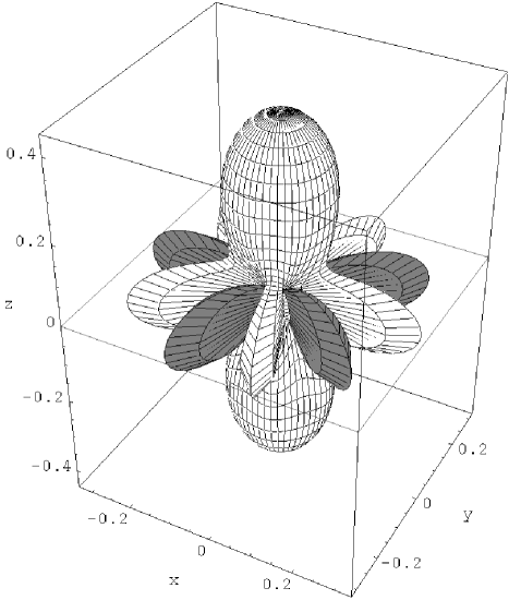
FIG. 1.: Wigner function for a polar cat state, Eq. (14) for the case of $N=5$ atoms. The absolute value of the function is measured along the radius in the direction $(\theta,\phi)$, and the surface is shown in light where the function is positive and in dark where it takes on negative values.

III Nonpolar cat states, and their squeezing properties

A Nonpolar cat states

One can also construct more general SC states by taking the superposition of any two atomic coherent states. An atomic coherent state (a quasiclassical state) [18], $\left|\tau\right\rangle$ is an eigenstate with the highest eigenvalue $m=j$ of the component of the angular momentum operator ‘pointing in the direction ${\bf n}$’:

$$\left({\bf J\cdot n}\right)|\tau\rangle=j|\tau\rangle.$$ (15)

The notation $\tau$ refers to a specific parametrization of the unit vector ${\bf n}$ by its stereographic projection to the complex plane. It is connected with the polar angle $\beta$ and the azimuth $\alpha$ of the direction ${\bf n}$ as $\tau=\tan(\beta/2)e^{-i\alpha}$. The atomic coherent state can be expanded in terms of the eigenstates $\left|j,m\right\rangle$ of $J_{z}$ [18]:

$$|\tau\rangle = \left(\frac{1}{1+|\tau|^{2}}\right)^{j}e^{\tau J_{+}}\left|j,-j\right\rangle=\sum_{m=-j}^{j}{2j\choose j+m}^{1/2}\frac{\tau^{j+m}}{(1+|\tau|^{2})^{j}}\left|j,m\right\rangle$$ (16)

$$= \sum_{m=-j}^{j}{2j\choose j+m}^{1/2}\sin^{j+m}(\beta/2)\cos^{j-m}(\beta/2)e^{-i(j+m)\alpha}\left|j,m\right\rangle.$$ (17)

The superposition of two quasiclassical coherent states is given by the ket:

$$|\Psi_{12}\rangle={\frac{{|\tau_{1}\rangle+|\tau_{2}\rangle}}{\sqrt{2(1+\text{Re}\langle\tau_{1}|\tau_{2}\rangle)}}}.$$ (18)

Recently Agarwal, Puri and Singh [13] and Gerry and Grobe [14] have proposed methods to generate such states in a cavity, via a dispersive interaction with the cavity mode.

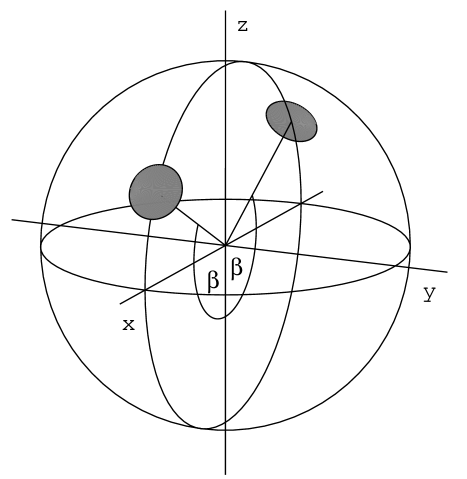
FIG. 2.: The phase space scheme of a nonpolar cat state, Eq.(18) with $\tau_{2}=-\tau_{1}$.

We choose here $\tau_{1}=\tan(\beta/2)$, $\tau_{2}=-\tau_{1}$. Then $\beta$ is the polar angle of the classical Bloch vector corresponding to the atomic coherent state ${|\tau_{1}\rangle}$ ($\beta$ is measured from the south pole), see Fig. 2. This means that the $x$ component of the expectation value of the dipole moment in these states is proportional to $\pm(N/2)\sin\beta$, respectively, and the $y$ component is zero. Any other equal weight superposition of two atomic coherent states can be obtained from this special choice by an appropriate rotation. The polar cat state of the previous section corresponds to the special case when the two points are the northern and southern poles of the Bloch sphere. If the centres of the two coherent states in question are not in opposite points of the sphere, then we will call their superposition as “nonpolar” cat states.

The corresponding quasiprobability distribution functions still can be explicitly calculated. For the Wigner function of the cat state $|\Psi_{12}\rangle$ one gets the following expression:

$$W(\theta,\phi)=\sqrt{\frac{N+1}{4\pi}} \sum_{K=0}^{2j}\sum_{Q=-K}^{K}{\frac{\sqrt{2K+1}{(2j)!}}{{2(1+(\cos\beta)^{2j})}}}{\ }\sum_{m=-j}^{j}{\frac{(-1)^{j-Q-m}+(-1)^{3j+m}+(-1)^{2j}+(-1)^{2j-Q}}{\sqrt{(j+m)!(j-m)!(j+Q+m)!(j-Q-m)!}}}\hfill$$ (22)

$$\times\left(\begin{array}[]{ccc}j&\ K&\ j\\ -m-Q&Q&m\end{array}\right)(\sin{\beta/2})^{2(j+m)+Q}(\cos{\beta/2})^{2(j-m)-Q}\ Y_{KQ}(\theta,\phi).$$

We present polar plots of this Wigner function in Fig. 3. for $N=5$ atoms and for several values of $\beta$.

FIG. 3.: Wigner functions for the state $|\Psi_{12}\rangle$ for $N=5$ atoms, and for several different values of $\beta$: (a) $\beta=20^{\circ}$, (b) $\beta=45^{\circ}$, (c) $\beta=55^{\circ}$, (d) $\beta=70^{\circ}$. For smaller values of $\beta$ the state goes over into a single coherent state, and then it has essentially only one positive lobe. This graphical presentation shows qualitatively that the $y$ component of the dipole moment is squeezed, the maximal value of the squeezing in the present case ($N=5$) comes about $\beta=43^{\circ}$.

For small $\beta$ values, the interference is weak and the maximum of the Wigner function is around $\theta=0$. For larger $\beta$-s the function has two maxima around $\theta=\pm\beta$, and the interference gets more pronounced. When $\beta=\pi/2$, the two maxima corresponding to the individual coherent states point in the $x$ and $-x$ directions, respectively. In this case we get back the Wigner function of the SC state of Eq. (1), rotated around the $y$ axis by $\pi/2$.

B Squeezing properties

The expectation values of the dipole operators $J_{x}$ and $J_{y}$ are zero in the state (18) with $\tau_{1}=\tan(\beta/2)$, $\tau_{2}=-\tau_{1}$, which is a consequence of the mirror symmetry of this state with respect of both the $x-z$ and the $y-z$ planes. As it is known, the variances of the dipole operators, $J_{x}$ and $J_{y}$ are equal to each other in an atomic coherent state:

$$(\Delta J_{x})^{2}|_{\left|\tau\right\rangle}=(\Delta J_{y})^{2}|_{\left|\tau\right\rangle}=j/2.$$ (23)

In order to calculate the variances in the state (18), one can use directly expansion (17) and the known matrix elements of $J_{x}$ and $J_{y}$, but the summations that occur are rather cumbersome to evaluate. A more effective procedure is to apply the method of generating functions [18]. All the necessary expectation values in a cat state can be calculated by the formula :

$$\left[\left(\frac{\partial}{\partial\xi}\right)^{a}\left(\frac{\partial}{\partial\eta}\right)^{b}\left(\frac{\partial}{\partial\zeta}\right)^{c}X_{A}\right]_{\xi=\eta=\zeta=0}=\left\langle\tau_{1}\right|J_{-}^{a}J_{z}^{b}J_{+}^{c}\left|\tau_{2}\right\rangle,$$ (24)

where

$$X_{A}(\xi,\eta,\zeta) \equiv \left\langle\tau_{1}\right|e^{\xi J_{-}}e^{\eta J_{z}}e^{\zeta J_{+}}\left|\tau_{2}\right\rangle=\frac{\left\langle-j\right|e^{(\tau_{1}^{*}+\xi)J_{-}}e^{\eta J_{z}}e^{(\tau_{2}+\zeta)J_{+}}\left|-j\right\rangle}{\{(1+|\tau_{1}|^{2})(1+|\tau_{2}|^{2})\}^{j}}$$ (25)

$$= \frac{\{e^{-\eta/2}+e^{\eta/2}(\tau_{1}^{*}+\xi)(\tau_{2}+\zeta)\}}{\{(1+|\tau_{1}|^{2})(1+|\tau_{2}|^{2})\}^{j}}^{2j}$$ (26)

is the (antinormally ordered) generating function.

Inserting the necessary operators, we obtain the following expressions for the variances in the state given by (18):

$$(\Delta J_{x})^{2}={\frac{j}{2}}\left(1+{\frac{(2j-1)\sin^{2}\beta}{{1+(\cos\beta)^{2j}}}}\right),$$ (27)

$$(\Delta J_{y})^{2}={\frac{j}{2}}\left(1-{\frac{(2j-1)(\cos\beta)^{2j-2}\sin^{2}{\beta}}{{1+(\cos\beta)^{2j}}}}\right).$$ (28)

Comparing these results with Eq. (23), we see, that except for some special cases the $J_{y}$ quadrature is squeezed while the $J_{x}$ quadrature is stretched in this state. The reason of this asymmetry lies in the fact, of course, that in the superposition (18) we have chosen states that are both centered in points lying in the $x-z$ plane.

One of the exceptional cases that is not squeezed is, if there is only one atom: $j=1/2.$ As it is easily seen, for $j=1/2$ any state in the two-dimensional Hilbert space is a coherent state, and therefore it does not show squeezing. The two other exceptions are $\beta=0$ for any $j$, because then the two coherent states coincide, and $\beta=\pi/2$, which is the rotated version of the polar cat state.

Writing Eq.(28) in the form $(\Delta J_{y})^{2}={j}(1-{\cal{S}})/2$, we can define the quantity ${\cal{S}}$ as the measure of squeezing. Analysis shows that if $N$ is large enough, then the maximum value of ${\cal{S}}$ is $0.56$ and it is achieved around $\beta_{m}=1.6/\sqrt{N}$. Figure 4 shows the dependence of ${\cal{S}}$ on $\beta$ for several values of $N=2j$.

FIG. 4.: The $\beta$ dependence of the quantity ${\cal{S}}$ in $(\Delta J_{y})^{2}=j(1-{\cal{S}}(\beta,j))/2$, for several values of $N=2j$. ${\cal{S}}$ can be considered as the measure of squeezing for a cat state consisting of two atomic coherent states separated by the central angle $2\beta$ on the Bloch sphere.

IV Decoherence and dissipation

As we mentioned in the Introduction, there have already been realizable methods proposed for the experimental generation of atomic SC states in a collection of two-level atoms [13, 14]. However, such an atomic ensemble can never be perfectly isolated from the surrounding environment. Further, any observation of these states necessarily leads to the interaction of the atomic system with a measuring apparatus. In both of these cases the atomic system interacts with a system containing a large number of degrees of freedom. A possible and successful approach to this problem [36] considers that the static environment continously influences the dynamics of the atomic subsystem, which besides exchanging energy with the environment loses the coherence of its quantum superpositions and evolves into a classical statistical mixture.

In this section we investigate the decoherence and dissipation of the atomic Schrödinger cat states embedded in an environment with many degrees of freedom, by writing down the master equation for the reduced density operator of the atomic subsystem. We provide the solution for the polar cat states (1).

A Model and solution

We couple our ensemble of two-level atoms to the environment which is supposed to be a multimode electromagnetic radiation with photon annihilation and creation operators $a_{k}$ and $a_{k}^{\dagger}$. Then the interacting system can be described by the following well known model Hamiltonian which considers dipole interaction and uses the rotating wave approximation:

$$H=\omega_{\text{a}}J_{z}+\hbar\sum_{k}\omega_{k}a_{k}^{\dagger}a_{k}+\sum_{k}g_{k}\left(a_{k}^{\dagger}J_{-}+a_{k}J_{+}\right),$$ (29)

where $\omega_{\text{a}}$ is the transition frequency between the two atomic energy levels, the $\omega_{k}$ denote the frequencies of the modes of the environment and $g_{k}$ are the coupling constants. If we suppose the environment to be in thermal equilibrium at temperature $T$, then the time evolution of the atomic subsystem is determined by a master equation for its reduced density operator $\rho(t)$ [32, 33]:

$$\hbar^{2}\frac{\text{d}\rho(t)}{\text{d}t}=-\frac{\gamma}{2}\ (\langle n\rangle+1)\ (J_{+}J_{-}\rho(t)+\rho(t)J_{+}J_{-}-2J_{-}\rho(t)J_{+})-\frac{\gamma}{2}\ \langle n\rangle\ (J_{-}J_{+}\rho(t)+\rho(t)J_{-}J_{+}-2J_{+}\rho(t)J_{-})$$ (30)

which involves the usual Born-Markov approximation and is written in the interaction picture. Here $\langle n\rangle=\left(\exp\left(\hbar\omega_{\text{a}}/(k_{\text{B}}T)\right)-1\right)^{-1}$ is the mean number of photons in the environment and $\gamma=(g(\omega_{\text{a}})\sigma(\omega_{\text{a}}))^{2}$ denotes the damping rate, where $\sigma$ is the mode density of the environment.

Eq. (30) can be obtained also in a somewhat different context, as described in [34]. Then one assumes the atomic subsystem to be placed in a resonant cavity with low quality mirrors causing the damping of the cavity mode at a rate $\kappa$. Under certain reasonable assumptions one can get Eq. (30) with $\gamma=2\,g(\omega_{\text{a}})^{2}/\kappa$.

From Eq. (30) one can easily deduce the following equations for the matrix elements of the density operator $\rho_{m,l}(t)\equiv\left\langle j,m\left|\rho(t)\right|j,l\right\rangle$:

$$\frac{\text{d}\rho_{m,l}(t)}{\text{d}t} = -\frac{\gamma}{2}\,[\,\langle n\rangle\left(2j(j+1)-m(m+1)-l(l+1)\right)+(\langle n\rangle+1)\left(2j(j+1)-m(m-1)-l(l-1)\right)\,]\,\rho_{m,l}(t)$$ (33)

$$+\,\gamma\,\langle n\rangle\,\sqrt{\left(j(j+1)-m(m-1)\right)\left(j(j+1)-l(l-1)\right)}\ \rho_{m-1,l-1}(t)$$

$$+\,\gamma\,(\langle n\rangle+1)\,\sqrt{\left(j(j+1)-m(m+1)\right)\left(j(j+1)-l(l+1)\right)}\ \rho_{m+1,l+1}(t).$$

Thus the time evolution of a particular density matrix element is coupled only to the two neighbouring elements in the corresponding diagonal for $\langle n\rangle>0$, and only to the neighbour with larger index at zero temperature.

In the case of a polar cat state (consisting of $N=2j$ atoms), the elements of the density matrix have zero initial values except for $\rho_{-j,-j},\ \rho_{j,j},\ \rho_{-j,j}$ and $\rho_{j,-j}\ (=\rho_{-j,j}^{*}).$ This implies that the density matrix elements, except for those in the main diagonal and for $\rho_{-j,j}$ and $\rho_{j,-j}$, remain identically zero for any time. Setting $\gamma=1$ (i.e. the time unit is $1/\gamma$) the equations for the elements in the main diagonal of the density matrix are the following:

$$\frac{\text{d}\rho_{m,m}(t)}{\text{d}t} = -\left[\langle n\rangle\,\left(j(j+1)-m(m+1)\right)+(\langle n\rangle+1)\left(j(j+1)-m(m-1)\right)\right]\ \rho_{m,m}(t)$$ (36)

$$+\ \langle n\rangle\,\left(j(j+1)-m(m-1)\right)\ \rho_{m-1,m-1}(t)$$

$$+\ (\langle n\rangle+1)\,\left(j(j+1)-m(m+1)\right)\ \rho_{m+1,m+1}(t)$$

with the initial values $\rho_{m,m}(t=0)=\frac{1}{2}(\delta_{m,j}+\delta_{m,-j})$ (cf. equation (1)). The dynamics of $\rho_{-j,j}$ is governed by the particularly simple equation:

$$\frac{\text{d}\rho_{-j,j}(t)}{\text{d}t}=-j(2\langle n\rangle+1)\rho_{-j,j}(t),$$ (37)

yielding immediately the following solution with the initial value $\rho_{-j,j}(0)=1/2$ corresponding to the polar cat state:

$$\rho_{-j,j}(t)=\frac{1}{2}\exp\left(-j(2\langle n\rangle+1)t\right).$$ (38)

As expected, the stationary solution of Eq. (36) is the Boltzmann distribution of the stationary values $\bar{\rho}_{m,m}$:

$$\bar{\rho}_{m,m} = \exp\left(-(m+j)\frac{\hbar\omega_{\text{a}}}{k_{\text{B}}T}\right)\frac{1-\exp\left(-\hbar\omega_{\text{a}}/(k_{\text{B}}T)\right)}{1-\exp\left(-(2j+1)\hbar\omega_{\text{a}}/(k_{\text{B}}T)\right)}=\frac{\left(\langle n\rangle/(\langle n\rangle+1)\right)^{m+j}}{(\langle n\rangle+1)\ \left(1-\left(\langle n\rangle/(\langle n\rangle+1)\right)^{2j+1}\right)}.$$ (39)

Approximate analytical time dependent solutions of Eq. (36) can be found especially for the case of superradiance, when $\rho_{j,j}(0)=1$ in [35], see also [12] and references therein. For the initial conditions corresponding to the polar cat state, the time dependent solution of equations (36) at zero temperature ($\langle n\rangle=0$) can be obtained by the following recursive integration:

$$\rho_{j,j}(t) = \frac{1}{2}\exp\left(-2jt\right),$$ (40)

$$\rho_{m,m}(t) = \exp\left(-b_{m}t\right)\left(\frac{1}{2}\ \delta_{m,-j}+b_{m+1}\int\limits_{0}^{t}\exp\left(b_{m}t^{\prime}\right)\ \rho_{m+1,m+1}(t^{\prime})\ \text{d}t^{\prime}\right),\hskip 28.45274pt-j\leq m<j$$ (42)

where $b_{m}=j(j+1)-m(m-1)$. These equations show rather explicitly, how does the initial excitation cascade down to the zero temperature stationary state.

For non-zero temperatures ($\langle n\rangle>0$) we have solved equations (36) numerically. We are going to analyze the solutions in the next subsection.

B Characteristic times

Figure 5 shows the time evolution of the relevant density matrix elements $\rho_{m,m}(t)$, $m=-j,-j+1,\ldots,j$ (solid lines) and $\rho_{-j,j}(t)$ (dashed line), in the case of initial polar cat states consisting of 5 and 50 atoms, for $\langle n\rangle=0,\ 1,\ 10$.

The actual value of $\rho_{-j,j}(t)$ characterizes the coherence of the corresponding state, since $\rho_{-j,j}$ and $\rho_{j,-j}$ ($=\rho_{-j,j}^{*}$) are the only nonzero matrix elements outside the main diagonal. Their exponential decay (cf. Eq. (38)) is the decoherence, shown by the dashed lines in the plots of Fig. 5. Thus it is reasonable to define the characteristic time of the decoherence by

$$t_{\text{dec}}=\frac{2}{N(2\langle n\rangle+1)},$$ (43)

implying $\rho_{-j,j}(t_{\text{dec}})=\rho_{-j,j}(0)/e$.

In contrast to the simple time dependence of $\rho_{-j,j}(t)$, the dynamics of the main diagonal elements $\rho_{m,m}(t)$ depend on the actual value of $\langle n\rangle$ and $N$ rather sensitively. The zero temperature cases, Fig. 5 (a) and (d), clearly show the initial excitation, contained in $\rho_{j,j}(0)=1/2$, cascading down to $\rho_{-j,-j}(\infty)=1$ as given by Eqs. (LABEL:recursion). At nonzero temperatures ($\langle n\rangle>0$) the time evolution of the $\rho_{m,m}(t)$-s is more complicated because of the coupling to both neighbours, cf. Eq. (33).

More information can be extracted from the time evolution of the $\rho_{m,m}(t)$-s by calculating the energy of the atomic subsystem as the function of time:

$$E(t)\equiv\langle\omega_{\text{a}}\,J_{z}\rangle(t)=\omega_{\text{a}}\text{Tr}\left(\rho(t)\,J_{z}\right)=\hbar\omega_{\text{a}}\sum_{m=-j}^{j}\,m\,\rho_{m,m}(t).$$ (44)

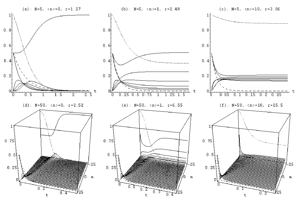
FIG. 5.: Plots of the density matrix elements $\rho_{m,m}(t)$, $m=-j,-j+1,\ldots,j$ (solid lines) and $\rho_{-j,j}(t)$ (dashed line) versus time (the time unit is $1/\gamma$). Plots are given for $N=5$ atoms: (a, b, c), and $N=50$ atoms: (d, e, f), for $\langle n\rangle=0$ (zero temperature): (a, d), for $\langle n\rangle=1$: (b, e), and for $\langle n\rangle=10$: (c, f). The solid lines may be identified as follows: in (a) the smaller $m$ is the later the corresponding $\rho_{m,m}$ has its maximal value; in (b) and (c) the stationary values of the $\rho_{m,m}$-s follow the Boltzmann distribution, see Eq. (39). In (d, e, f) the $\rho_{m,m}$-s follow each other along the axis labeled by the $m$. The dotted lines (starting from 1 at $t=0$) show the normalized energy of the atomic subsystem $1+E(t)/(-j\hbar\omega_{\text{a}})$, see Eq. (44). The number $r=t_{\text{diss}}/t_{\text{dec}}$ is the ratio of the characteristic time of dissipation to the characteristic time of decoherence.

The process of dissipation (i.e. the change of the energy of the atomic subsystem in time) can be very easily followed by studying $E(t)$. This function, normalized to the zero temperature stationary energy and shifted to vary from 1 to its stationary value: $1+E(t)/(-j\hbar\omega_{\text{a}})$, is shown in the plots of Fig. 5 by the dotted lines. Since its asymptotic behavior is exponential-like, it is reasonable to define the characteristic time of dissipation $t_{\text{diss}}$ by requiring

$$|E(t_{\text{diss}})-E(\infty)|=|E(0)-E(\infty)|/e.$$ (45)

In order to ensure that $E(t)$ achieves its stationary value with a good accuracy in the plots of Fig. 5 we have set the time range to $5\,t_{\text{diss}}$. It is seen that the value of $r=t_{\text{diss}}/t_{\text{dec}}$ grows with both the temperature and the number of atoms. A more detailed analysis of this question follows later in this section.

The initial state of the process, the polar cat state, has sharply non-classical features. On the other hand, at non-zero temperature the final stationary state of the present model is a thermal state, which is classical in its nature. (At zero temperature the stationary state is also non-classical, since it is the state $|j,-j\rangle$.) It is natural to ask, when does the transition from the non-classical to the classical stage occur? What is a good measure of non-classicality reflecting the change of non-classical nature of the corresponding state?

The spherical Wigner function (6) provides a good answer to both of these questions. Quantum states are generally considered essentially non-classical if the corresponding Wigner function takes on also negative values. Therefore to answer the second question, for the measure of the degree of non-classicality we propose to use the quantity $\nu=1-(I_{+}-I_{-})/(I_{+}+I_{-})$, where $I_{+}$ is the integral of the Wigner function over those domains where it is positive while $I_{-}$ is the absolute value of the integral of the Wigner function over the domains where it is negative. Since the integral of the Wigner function over the sphere is 1, $I_{+}-I_{-}=1$, thus $\nu=2I_{-}/(2I_{-}+1)$, and it is easy to see that $0\leq\nu<1$. According to this definition, the bigger is the value of $\nu$, the more non-classical is the state, and for all classical states one has $\nu=0$.

Regarding now the first question, namely for how long is the state of the atomic system non-classical, we introduce a third kind of characteristic time $t_{\text{ncl}}$. We define $t_{\text{ncl}}$ to be the time instant when the corresponding spherical Wigner function becomes non-negative everywhere on the sphere, i.e. $\nu$ becomes 0. We will return to this question in connection with the time evolution of the Wigner function, which we will present in the next subsection in more detail.

Based on the information provided by the three kinds of characteristic times, we consider here the dependence of the process on the number of atoms and on the temperature. In Figure 6 we plot $t_{\text{diss}}$ (dashed line), $t_{\text{dec}}$ (solid line) and $t_{\text{ncl}}$ (dotted line) as the function of the number of constituent atoms of the polar cat $N$, for several temperatures, on a log-log scale.

FIG. 6.: Plots of the characteristic times of decoherence, $t_{\text{dec}}$ (solid line), dissipation, $t_{\text{diss}}$ (dashed line) and non-classicality, $t_{\text{ncl}}$ (dotted line) versus the number of atoms, on a log-log scale. The uppermost solid and dashed line are for $\langle n\rangle=0$ (there is no plot for $t_{\text{ncl}}$ at zero temperature, since the state stays non-classical), while the subsequent groups of the three kinds of lines, one under the other, are for $\langle n\rangle=1,\ 10,\ 100$, respectively.

It is seen that the characteristic time of decoherence $t_{\text{dec}}$ is inversely proportional to the number of atoms (the straight solid lines in Fig. 6), according to the definition (43). Compared to this, the characteristic time of non-classicality $t_{\text{ncl}}$ decreases less rapidly with increasing number of atoms. The characteristic time of dissipation $t_{\text{diss}}$ first slightly increases at non-zero temperature then it achieves a maximum which depends on $\langle n\rangle$ and finally it decreases nearly inversely proportional to the number of atoms. The values of $t_{\text{diss}}$ at different temperatures seem to converge slowly beyond a certain number of atoms.

It seems however rather surprising that the ratio $t_{\text{diss}}/t_{\text{dec}}$ is not as large as such a quantity is usually expected to be [36, 37]: in the case of $N=1000$ it is 4.04 for $\langle n\rangle=0$, and it is still just around 350 for $\langle n\rangle=100$. (Note that $\langle n\rangle=100$ corresponds to a temperature of 250 K in the case of typical experiments [4].) The ratio $t_{\text{diss}}/t_{\text{dec}}$ seems not even to vary considerably with increasing $N$ beyond the maximum of $t_{\text{diss}}$ mentioned above. Thus the process of decoherence is extremely slow in the case of a polar cat state which is coupled to the environment by an interaction leading to the master equation (30).

Similar effects have already been reported for other physical systems earlier [38]. In a recent work Braun, Braun and Haake [39] investigated the decoherence of an atomic SC state $|\tau_{1}\rangle+|\tau_{2}\rangle$ based on Eq. (30) for zero temperature. By evaluating a certain quantity characterising the decoherence rate at the initial time, and applying a semiclassical procedure for finite times they concluded that for atomic SC states with $\tau_{1}\tau_{2}^{*}=1$ the decoherence slows down.

Our initial state, the polar cat state fulfils the former condition. The results presented in Fig. 6 derive from the solution of the master equation for the whole process. They are in agreement with the statements of Ref.[39], where the initial stage of the decoherence is analyzed for the case of zero temperture.

C Wigner functions

We illustrate now the process of decoherence and dissipation using the spherical Wigner function (6).

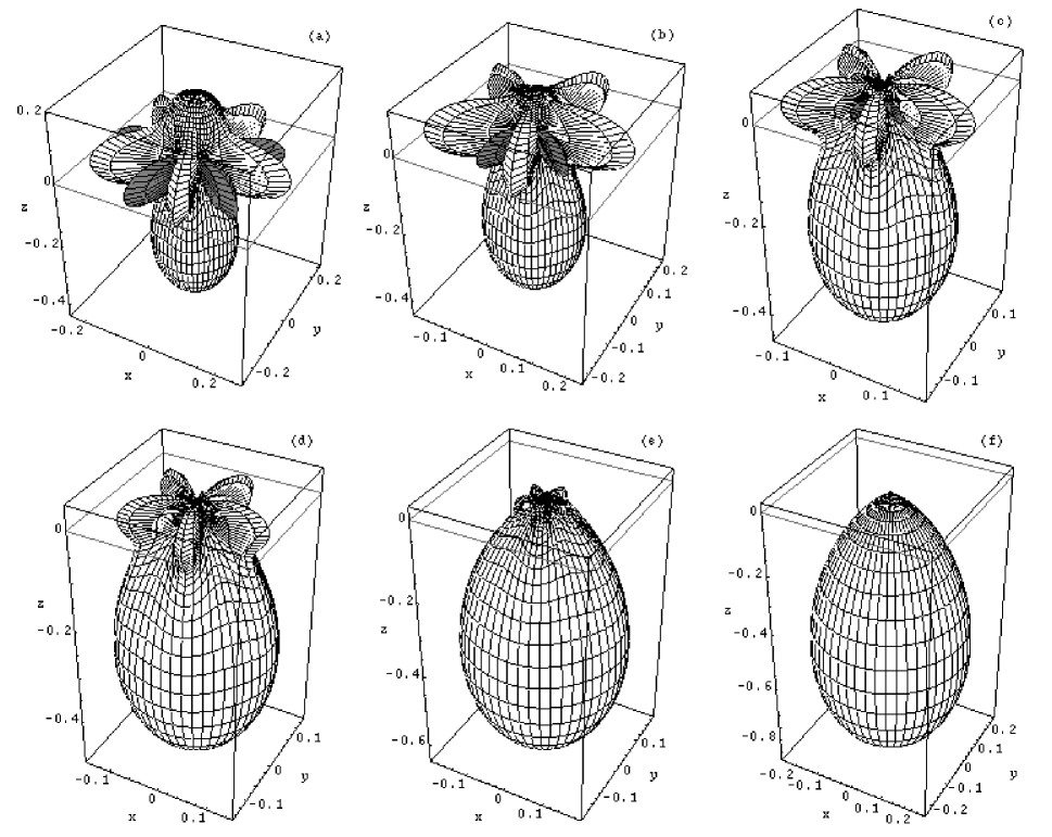
FIG. 7.: Polar plots of the temporal change of the Wigner function representing the decoherence and dissipation of the initial polar cat state (1), made of 5 atoms and shown in Fig. 1, at zero temperature. The dynamics of the corresponding density matrix elements is shown in Fig. 5(a). The time instants are the following (in units of $1/\gamma$): (a) 0.1, (b) 0.2, (c) 0.4 ($=t_{\text{dec}}$), (d) 0.506 ($=t_{\text{diss}}$), (e) 0.8, (f) 2.5.

In order to obtain its time dependence we have to calculate first the characteristic matrix $\varrho_{K,Q}(t)=\text{Tr}\left(\rho(t)T_{K,Q}^{\dagger}\right)$ from the matrix elements $\rho_{m,l}(t)$ according to

$$\varrho_{K,Q}(t)=\sqrt{2K+1}\sum_{m=-j}^{j}(-1)^{j-m}\left(\begin{array}[]{ccc}j&K&j\\ -m&Q&m-Q\end{array}\right)\rho_{m,m-Q}(t).$$ (46)

From Eq. (46) it can be seen that only $\varrho_{K,0}$ ($K=0,1,\ldots,N$) and $\varrho_{N,N}=(-1)^{N}(\varrho_{N,-N})^{*}$ are nonzero. This fact (which is due to the initial conditions specified by the polar cat state) ensures that the azimuthal dependence of the spherical Wigner function is determined only by the real part of the spherical harmonic $Y_{N,N}(\theta,\phi)$ which is proportional to $\cos(N\phi)$. Therefore the Wigner function keeps its initial azimuthal symmetry during the whole process. Further, since $\varrho_{N,N}(t)=(-1)^{N}\rho_{j,-j}(t)$, the azimuthal modulation of the spherical Wigner function explicitly shows the degree of the coherence of the actual state.

Figures 7 and 8 show the polar plots of the spherical Wigner function transforming its shape in time at $\langle n\rangle=0$ and $\langle n\rangle=10$, respectively. The initial state is a polar cat made of $N=5$ atoms and its Wigner function is shown in Fig. 1.

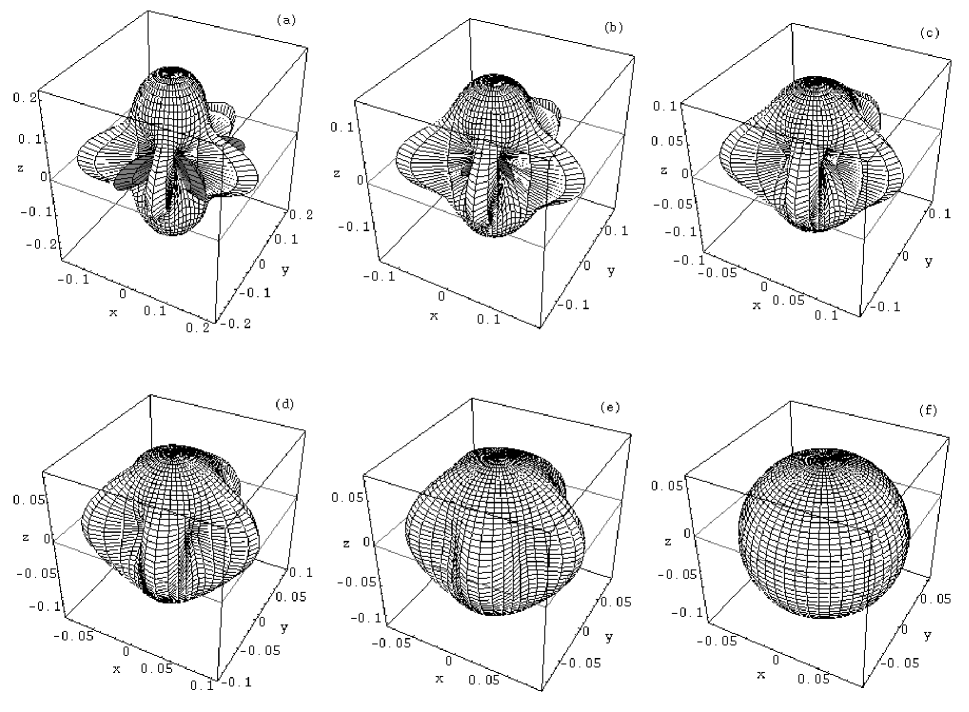
FIG. 8.: Polar plots of the temporal change of the Wigner function representing the decoherence and dissipation of the initial polar cat state (1), made of 5 atoms and shown in Fig. 1, for $\langle n\rangle=10$. The dynamics of the corresponding density matrix elements is shown in Fig. 5(c). The time instants are the following (in units of $1/\gamma$): (a) 0.01, (b) 0.019 ($=t_{\text{dec}}$), (c) 0.031 ($=t_{\text{ncl}}$), (d) 0.045, (e) 0.058 ($=t_{\text{diss}}$), (f) 0.25.

In Figures 7 and 8 the following main characteristics of the process can be identified. The decoherence is shown by the decreasing and finally disappearing ripples along the equator. The vanishing of non-classicality, i.e. the decrease of the parameter $\nu$, can be easily recognized as the decrease of the negative (dark) wings. At nonzero temperature they disappear exactly at $t_{\text{ncl}}$, as shown in Fig. 8(c). The dissipation is represented by the approach of the initial upper and lower bumps to each other. At zero temperature (Fig. 7) the upper bump disappears and goes over to the lower one. This stationary shape of the Wigner function corresponds to the lowest coherent state $|j,-j\rangle$ [30]. For $\langle n\rangle=10$, when the stationary energy is close to the initial energy, not only the upper bump moves downwards but also the lower one lifts upwards. The stationary Wigner function has nearly a spherical symmetry, although its center is not in the origin.

In agreement with Fig. 6, the plots of Figures 7 and 8 show, that the timescales of the decoherence and of the dissipation are very close to each other in the case of 5 atoms, for zero temperature they are practically the same. Then the spherical Wigner function exhibits considerable azimuthal modulation (ripples) also at $t_{\text{diss}}$.

We may come back finally to the question of finding the characteristic time of non-classicality $t_{\text{ncl}}$. According to the arguments given after Eq. (46) it is sufficient to study the Wigner function within a $\phi$-range of length $2\pi/N$, e.g. $0\leq\phi\leq 2\pi/N$, because it is invariant with respect of rotations by $\phi=k{2\pi\over N},\ (k=1,2,\dots,N)$ i.e. it has $C_{N}$ symmetry at all times. Therefore the spherical Wigner function of a polar cat state, while subject to dissipation and decoherence, has its minimum value always at $\phi=\pi/N$. Thus in order to calculate $t_{\text{ncl}}$, it is sufficient to follow the time evolution of the section $W(\theta,\phi=\pi/N)$. Further, in connection with the calculation of the measure of non-classicality $\nu$, it is sufficient to consider the above mentioned $\phi$-range when evaluating the integrals $I_{+}$ and $I_{-}$.

V Conclusions

We have considered a class of states in an ensemble of two-level atoms, a superposition of two distinct atomic coherent states which are called atomic Schrödinger cat states. According to the relative positions of the constituents we have defined polar and nonpolar cat states. We have investigated their properties based on the spherical Wigner function, which has been proven to be a convenient tool to investigate the quantum interference effects.

We have shown that nonpolar cat states generally exhibit squeezing, for which we have introduced the measure ${\cal S}$. The squeezing depends on the separation of the components of the cat and on the number of the atoms the cat is consisting of. By solving the master equation of this system embedded in an external environment we have determined the characteristic times of decoherence, dissipation and non-classicality of an initial polar cat state. We have shown how these depend on the number of the microscopic elements the cat consists of, and on the temperature of the environment. Our results show that the decoherence of the polar cat state is surprisingly slow: $t_{\text{diss}}/t_{\text{dec}}$ is less then a half of an order of magnitude for zero temperature, making these states potentially significant in several areas of quantum physics, e.g. experimental studies of decoherence, quantum computing and cryptography. We have visualised the process, governed by the interaction with the external environment, using the spherical Wigner function. Its transformation in time reflects the characteristics of the behaviour of the atomic subsystem in a suggestive way.

REFERENCES

- [1] E-mail address: benedict@physx.u-szeged.hu
- [2] E-mail address: czirjak@physx.u-szeged.hu
- [3] C. Monroe, D. M. Meekhof, B. E. King, D. J. Wineland, Science 272, 1131 (1996)
- [4] M. Brune, E. Hagley, J. Dreyer, X. Mâitre, A. Maali, C. Wunderlich, J. M. Raimond, and S. Haroche, Phys. Rev. Lett. 77, 4887 (1996)
- [5] B. Yurke, D. Stoler, Phys. Rev. Lett. 57, 13 (1986)
- [6] J. Janszky, A. Vinogradov, Phys. Rev. Lett 64, 2771 (1990)
- [7] W. Schleich, M. Pernigo, F. LeKien, Phys Rev. A 44, 2172 (1991)
- [8] V. Buzek, H. Moya-Cessa, P. L. Knight, S. D. L. Phoenix, Phys. Rev A 45, 5193 (1992)
- [9] J. Cirac, P. Zoller, Phys. Rev. A 50, R2799 (1994)
- [10] R. H. Dicke, Phys. Rev. 93, 99 (1954)
- [11] M. Gross, S. Haroche, Phys. Rep. 93, 301 (1982)
- [12] M. G. Benedict, A. M. Ermolaev, V. A. Malyshev, I. V. Sokolov, E. D. Trifonov, Superradiance (IOP, Bristol, 1996)
- [13] G. S. Agarwal, R. R. Puri, R. P. Singh, Phys. Rev A 56, 2249 (1997)
- [14] C. C. Gerry, R. Grobe, Phys. Rev A 57, 2247 (1998)
- [15] M. Freyberger, P. Bardroff, C. Leichtle, G. Schrade, W. Schleich, Physics World 10, (11) 41 (1997)
- [16] D. Leibfried, D. M. Meekhof, B. E. King, C. Monroe, W. M. Itano, D. J. Wineland, Phys. Rev. Lett. 77, 4281 (1996)
- [17] R. L. Stratonovich, Sov. Phys. JETP 31, 1012 (1956)
- [18] F. Arecchi, E. Courtens, R. Gilmore, H. Thomas, Phys. Rev. A 6, 2221 (1972)
- [19] G. S. Agarwal, Phys. Rev. A 24, 2889 (1981)
- [20] R. Gilmore J. Phys. A: Math. Gen. 9, L65 (1976)
- [21] J. C. Várilly, J. M. Gracia-Bondia, Ann. Phys. (NY) 190, 107 (1989)
- [22] M. O. Scully, K. Wódkiewicz, Found. Phys. 24, 85 (1994)
- [23] K. E. Cahill, R. J. Glauber, Phys. Rev. 177, 1857 and 1882 (1969)
- [24] G. S. Agarwal, E. Wolf, Phys. Rev. D 2 2161, 2187, and 2206 (1970)
- [25] P. Földi, M. G. Benedict and A. Czirják, Acta Phys. Slovaca 48, 335 (1998)
- [26] N. M. Atakishiyev, S. M. Chumakov, K. B. Wolf, J. Math. Phys. 39 6247 (1998)
- [27] C. Brif, A. Mann, J. Phys. A: Math. Gen. 31, L9 (1998); Phys. Rev. A. 59, 971 (1999)
- [28] A. Czirják, M. G. Benedict, Quantum Semiclass. Opt. 8, 975 (1996)
- [29] L. C. Biederharn, J. D. Louck, Angular Momentum in Quantum Physics (Addison-Wesley, Reading, MA, 1981)
- [30] J. Dowling, G. S. Agarwal, W. P. Schleich, Phys. Rev. A 49, 4101 (1994)
- [31] M. G. Benedict, A. Czirják, Cs. Benedek, Acta Physica Slovaca 47, 259 (1997)
- [32] G. S. Agarwal, in Springer Tracts in Modern Physics, Vol 70. (Springer, Berlin, 1974)
- [33] D. F. Walls, G. J. Milburn, Quantum Optics (Springer, Berlin, 1994)
- [34] R. Bonifacio, P. Schwendimann and F. Haake, Phys. Rev. A 4, 302 and 854 (1971)
- [35] V. Degiorgo, F. Ghielmetti, Phys. Rev. A 4, 2415 (1971); S. Haroche, in New trends in atomic physics, Les Houches Summer School Lecture Notes, session 38. Eds. R. Stora, G. Grynberg, (North Holland, Amsterdam, 1984)
- [36] W. H. Zurek, Phys. Rev. D 24, 1516 (1981);
- [37] A. O. Calderia, A. J. Leggett, Ann. Phys. (NY) 149, 374 (1983); D. F. Walls and G. J. Milburn, Phys. Rev. A 31, 2403 (1985); F. Haake, D. F. Walls, Phys. Rev. A 36, 730 (1987); F. Haake, M. Żukowski, Phys. Rev. A 47, 2506 (1993); W. T. Strunz, J. Phys. A: Math. Gen. 30, 4053 (1997);
- [38] C. C. Gerry, E. E. Hach III, Phys. Lett. A 174, 185 (1993); B. R. Garraway, P. L. Knight, Phys. Rev. A 49, 1266 (1994); Phys. Rev. A 50, 2548 (1994); R. L. de Matos Filho, W. Vogel, Phys. Rev. Lett. 76, 608 (1996); J. F. Poyatos, J. I. Cirac, P. Zoller, Phys. Rev. Lett. 77, 4728 (1996); D. A. Lidar, I. L. Chuang, K. B. Whaley, Phys. Rev. Lett. 81, 2594 (1998)
- [39] D. Braun, P. A. Braun and F. Haake, Slow Decoherence of Superpositions of Macroscopically Distinct States, in Proceedings of the 1998 Bielefeld conference on ’Decoherence: Theoretical, Experimental, and Conceptual Problems’, (Springer, Berlin); see also the Los Alamos e-print: quant-ph/9903040