Testing of quantum phase in matter wave optics

Abstract

Various phase concepts may be treated as special cases of the maximum likelihood estimation. For example the discrete Fourier estimation that actually coincides with the operational phase of Noh, Fougères and Mandel is obtained for continuous Gaussian signals with phase modulated mean. Since signals in quantum theory are discrete, a prediction different from that given by the Gaussian hypothesis should be obtained as the best fit assuming a discrete Poissonian statistics of the signal. Although the Gaussian estimation gives a satisfactory approximation for fitting the phase distribution of almost any state the optimal phase estimation offers in certain cases a measurable better performance. This has been demonstrated in neutron–optical experiment.

1 Introduction

Physics enables us to comprehend Nature by considering intimate relations between various effects. Any physical observation can always be compared and analyzed in relation with a particular internal model, providing us with some additional insight into the laws of Nature. However, this effort need not and usually does not tend to a unique solution. It may happen that there are several plausible models and the given observation is not able to discriminate among them. On the other hand it may also happen that some of the assumptions about the system need not to be apparent. Certain statements therefore pretend to be more general than they are in reality. This interplay between physics and philosophy may be demonstrated on the long standing problem of quantum theory–on the problem of quantum phase. Phase measurements belong to standard detection techniques revealing the wave property of the signal. The quantum phase, however, encountered theoretical difficulties when an adequate quantum theory has been constructed [1].

There are several concepts for the description of phase in quantum theory at present. For an up to date overview see [2, 3]. Some of them are accenting the theoretical aspects, other the experimental ones. The operational approach formulated by Noh, Fougères and Mandel (NFM) [4, 5] is motivated by the correspondence principle in classical wave theory. The interference pattern is adopted for the scheme where the $\sin$ and $\cos$ function of the phase shift are measured simultaneously in the 8-port homodyne detection. An equivalent measurement may be realized on the Mach-Zehnder interferometer, provided that the measurement of an unknown phase shift is done with and without an additional $\pi/2$ phase shifter. The NFM scheme is plausible whenever the signal behaves like a classical wave since besides the principle of correspondence, no other assumptions has been used.

As a particular result, the NFM scheme provides the optimum result, provided that the statistics of the signals is represented by Gaussian statistics with a phase sensitive mean and a phase insensitive noise. Since realistic signals in the quantum world do not meet these rather restricting criteria, phase prediction based on them is not optimum in general. The difference between Gaussian estimation and optimum treatments is caused by the statistical nature of the phenomena. This can be experimentally registered in an interferometer with discrete Poissonian signal. Several possible interpretations of this comparison are noteworthy: i) This may be considered as a testing of the operational quantum phase prediction. It quantifies how well the NFM phase concept fits reality. ii) It may be interpreted as a nontrivial statistically motivated “quantum calibration” of an interferometer. The visibility of interference fringes is usually used for this purpose. However, this criterion focusses on the wave property of the detected signal only. The proposed method involves and evaluates the whole detection process, particularly the ability to control phase shift in the experimental arrangement and the statistics of the detected signal. This seems to be in accordance with the pragmatic interpretation of quantum theory, where the results depend irreducibly on both state preparation and measurement. iii) In the framework of wave–particle duality, the proposed treatment tries to answer the question: “Does the interfering signal resemble more discrete particles or classical continuous waves ?” iv) It provides an example of indirect observation of several parameters. Particularly, by detecting the interference fringes, the phase shift as well as the visibility may be determined as fluctuating variables. It provides one of the simplest examples of the so called “quantum state reconstruction” procedure.

This paper is organized as follows. In the second section, the main idea of comparing the NFM scheme with an optimum phase prediction is developed. In the third section, the idea is generalized in order to apply the scheme for phase measurement in matter wave interferometry. The fourth section provides the experimental realization in neutron interferometry the results obtained.

2 Statistical formulation of operational phase concepts

In this section the operational phase concept will be naturally embedded into the general scheme of quantum estimation theory [6, 7]. A similar approach has been already used in [8, 9]. However, since the purpose of the detection scheme is to predict the phase shift after each run, the point estimators of phase corresponding to the maximum–likelihood (MaxLik) estimation will be used here [10, 11]. Assume an ideal device with four output channels enumerated by indices 3,4,5,6, where the actual values of intensities are registered in each run. The values fluctuate in accordance with the statistics of continuous Gaussian signals. The mean intensities are modulated by a phase parameter $\theta$ as

$$\bar{I}_{3,4}=\frac{I}{2}(1\pm V\cos\theta)$$

$$\bar{I}_{5,6}=\frac{I}{2}(1\pm V\sin\theta),$$ (1)

where $I$ and $V$ are total input intensity and visibility of the interference fringes, respectively. The energy is splitted symmetrically between all the output ports. This device represents nothing else than a classical wave picture of the original 8-port homodyne detection scheme. Equivalently, it also corresponds to a Mach-Zehnder interferometer, when the measurement is done for an unknown phase shift together with a zero and a $\pi/2$ auxiliary phase shifters. In this case, the data are not obtained simultaneously, but should be collected during repeated experiments. Provided that a particular combination of outputs $I_{3},I_{4},I_{5},I_{6}$ has been registered, the phase shift should be inferred. In accordance with the MaxLik approach [12], the sought-after phase shift is given by the value that maximizes the likelihood function. The likelihood function corresponding to the detection of given data reads

$${\cal L}(\theta)=\frac{1}{\sigma^{4}4\pi^{2}}\exp\left\{\frac{1}{2\sigma^{2}}\left({-[I_{3}-\bar{I}_{3}]}^{2}-{[I_{4}-\bar{I}_{4}]}^{2}-\right.\right.$$

$$\left.\left.{-[I_{5}-\bar{I}_{5}]}^{2}-{[I_{6}-\bar{I}_{6}]}^{2}\right)\right\}.$$ (2)

Here the variation $\sigma$ represents the phase insensitive noise of each channel. The sampling of intensities may serve for an estimation of phase shift, the average number of particles and the visibility simultaneously. A notation analogous to the definition of phase by Noh, Fougères and Mandel [5] can be introduced as

$$e^{i\theta_{NFM}}=\frac{I_{3}-I_{4}+i(I_{5}-I_{6})}{\sqrt{(I_{3}-I_{4})^{2}+(I_{5}-I_{6})^{2}}}$$ (3)

$$R=\sqrt{(I_{3}-I_{4})^{2}+(I_{5}-I_{6})^{2}}.$$ (4)

The likelihood function may be rewritten to the form

$${\cal L}(\theta,V,I)\propto \exp\bigl{\{}-\frac{1}{2\sigma^{2}}[I-\frac{1}{2}\sum_{i=3}^{6}I_{i}]^{2}\bigr{\}}$$

$$\times \exp\bigl{\{}-\frac{1}{4\sigma^{2}}[VI-R\cos(\theta-\theta_{NFM})]^{2}\bigr{\}}$$

$$\times \exp\bigl{\{}\frac{1}{4\sigma^{2}}R^{2}\cos^{2}(\theta-\theta_{NFM})\bigr{\}}$$

and is maximized by the choice of parameters

$$\theta=\theta_{NFM},$$ (6)

$$V=\min\biggl{(}\frac{2R}{\sum_{i=3}^{6}I_{i}},1\biggr{)},$$ (7)

$$I=\frac{1}{2}\sum_{i=3}^{6}I_{i}.$$ (8)

Hence the operational phase concept of Noh, Fougères and Mandel is nothing but the MaxLik estimation for waves represented by continuous Gaussian signal with phase–independent and symmetrical noises. These rather strong assumptions are associated with the behaviour of waves in classical field theory.

Since realistic signals are discrete they meet neither of these criteria and therefore, deviations in the optimum phase prediction should be expected. Assume the Poissonian statistics of an ideal laser. Together with the phase, all the parameters which are not controlled in the experiment will be optimally predicted as well. Denote for concreteness the detected discrete values as numbers $n_{3},n_{4},n_{5},n_{6}.$ The likelihood function corresponding to this particular detection as a function of the parameters $\theta,V$ and $N$ reads

$${\cal L}(\theta,V,N)\propto\left(\frac{N}{2}\right)^{n_{3}+n_{4}+n_{5}+n_{6}}e^{-2N}(1-V\cos\theta)^{n_{3}}$$

$$\times(1+V\cos\theta)^{n_{4}}(1-V\sin\theta)^{n_{5}}(1+V\sin\theta)^{n_{6}}.$$ (9)

The MaxLik estimation for parameters gives the optimum values for the phase shift, the visibility and the mean particle number as

$$e^{i\theta}=\frac{1}{V}\left[\frac{n_{4}-n_{3}}{n_{4}+n_{3}}+i\frac{n_{6}-n_{5}}{n_{6}+n_{5}}\right],$$ (10)

$$V~{}=\sqrt{{\left(\frac{n_{4}-n_{3}}{n_{4}+n_{3}}\right)}^{2}+{\left(\frac{n_{6}-n_{5}}{n_{6}+n_{5}}\right)}^{2}},$$ (11)

$$N=\frac{n_{3}+n_{4}+n_{5}+n_{6}}{2}.$$ (12)

These relations provide a correction of the Gaussian wave theory with respect to the discrete signals. Besides the phase shift, the visibility of the interference fringes and the total energy input can be evaluated simultaneously.

An apparent difference between relations (6–8) and (10–12) represents the theoretical background of the presented treatment. Adopting the interpretation of Ref. [5], in both these approaches the unnormalized $\cos$ and $\sin$ functions of the phase shift are detected. However, the normalizations differ in both approaches. In the former Gaussian case, the normalization is performed only once, whereas in the latter Poissonian case it is done in two steps. The $\cos$ and $\sin$ functions of phase are normalized separately with respect to the total number of particles on both the output ports and then again among themselves. Obviously, both predictions will coincide provided that there is almost no information available in the low field limit $I,N\rightarrow 0.$ Similarly in the strong field limit $I,N\rightarrow\infty,$ where any statistics approaches the Gaussian one, the differences must disappear. Possible deviations may appear in the intermediate regime, characterized approximately by conditions $I,N\approx O(1).$ The test of the difference between $(\ref{NFM1})$ and $(\ref{max1})$ is proposed as controlled phase measurement. The phase difference may be adjusted to a certain value and estimated independently using both the methods $(\ref{NFM1})$ and $(\ref{max1})$ in repeated experiments. The efficiency of both methods is then compared by evaluation of confidence intervals. Since any imperfections of the detection scheme will smoothen the differences, it is questionable whether both schemes can be experimentally distinguished. This idea will be pursued in the following sections.

Before doing this, the statistical analysis may clarify some subtle points of the NFM treatment, particularly then the nature of discarded data. Obviously the data yielding the ambiguous phase $e^{i\theta_{NFM}}=0/0$ in equation (6) would provide zero visibility for both (7) and (11). For a more detailed analysis, the Bayes theorem may be applied as well. In this case the likelihood functions quantifies the phase information involved in the detected data as posterior phase distribution. Gaussian statistics provides homogeneous posterior phase distribution, whereas Poissonian statistics yields the four peak posterior distribution of the phase shift resembling effectively the homogeneous one. This statistical analysis supports the conclusion of Refs. [13, 14, 15] that the detected data cannot be discarded. Provided that some data are discarded, the average number of particles, i.e. the average energy corresponding to the phase detection changes. Particularly, provided that the experiment has been done $M$ times and a total number $M_{i}$ of particles has been detected in each run, the average number of particles is simply $\sum_{i,all}M_{i}/M.$ Provided that some data appearing $M_{d}$ times are discarded and not included in the evaluation the corresponding phase estimation is done with an average intensity loss $(\sum_{i,all}M_{i}-\sum_{i,disc}M_{i})/(M-M_{d}).$ Obviously, the measurement with and without discarding is done with a different energy input and this difference may be substantial. For example, this explains the ambiguity of the interpretation in Ref. [16]. When the phase of a quantum field is measured against a classical field, no data are discarded since the field is strong. The relative phase of two quantum fields may then be evaluated separately against a strong field and a difference of two such phases values provides the relative phase. However, this cannot be directly compared with direct measurements of two (weak) quantum fields against themselves, when some data are canceled. Although both measurements have been done with the same quantum states, the average energies of the corresponding phase detection may differ significantly. No wonder that the measurement with higher average energy gives better (sharper) results as observed in Ref. [16].

The analysis given here will be adopted to the case of neutron interferometry, when the number of particles can be detected and discriminated with high efficiency [17]. Highly efficient neutron detectors then provide almost perfect neutron number measurements. However the interference pattern exhibits lower visibility and the splitting process is far away from the symmetrical case. This will be taken into account when adopting the scheme to the case of neutron interferometry.

Analogous analysis for detection of light needs other modification. Since the efficiency of photodetection is less than unity, number of particles cannot be detected in such a straightforward way. Instead, the absence or presence of the week signal on the detector can be used for phase estimation. However, this will be dealt with separately in the forthcoming publication.

3 Phase estimation in neutron interferometry

Assume the following modification of the scheme developed above. The output ports of an interferometer are considered to be nonsymmetrical. The measurement is done with many auxiliary phase shifters. Neutron beams inside the perfect crystal neutron interferometer will be described at first as a classical wave. The signals $I_{j}^{o}$, $I_{j}^{h}$ detected at the two output ports $o$,$h$ (Fig. 1) are regarded as stochastic Gaussian intensities with phase sensitive means

$$\bar{I}_{j}^{o} = I^{o}+I^{V}\cos(\theta+\Delta_{j})$$

$$\bar{I}_{j}^{h} = I^{h}-I^{V}\cos(\theta+\Delta_{j}),$$ (13)

where $\theta$ is the true phase shift between the two branches of the interferometer, $I^{o}$ and $I^{h}$ are the mean intensities of the two interference fringes, $I^{V}$ stands for the modulation amplitude of the interference fringes (unnormalized visibility) and $\Delta_{j}$ are the values of the auxiliary shifts

$$\Delta_{j}=\frac{2\pi j}{N},\qquad j=0..N-1,\qquad N\in{\cal N}.$$ (14)

The Gaussian statistics of the detected signal yields its likelihood function in the form

$${\cal L}(\theta)\propto\exp\biggl{\{}-\frac{1}{2\sigma^{2}}\sum\limits_{j=0}^{N-1}\left[(I_{j}^{o}-\bar{I}_{j}^{o})^{2}+(I_{j}^{h}-\bar{I}_{j}^{h})^{2}\right]\biggr{\}}.$$ (15)

Introducing the complex parameter R as

$$R = \sum\limits_{j}(I_{j}^{o}-I_{j}^{h})\exp(-i\Delta_{j}),$$ (16)

the parameters maximizing the likelihood function read

$$e^{i\theta} = \frac{R}{|R|},$$ (17)

$$I^{o}=\frac{1}{N}\sum\limits_{j}I_{j}^{o},\qquad I^{h}=\frac{1}{N}\sum\limits_{j}I_{j}^{h},$$ (18)

$$I^{V} = \mbox{min}\biggl{\{}\frac{|R|}{N},I^{o},I^{h}\biggr{\}}.$$ (19)

The relation (19) follows from the condition of semidefiniteness of the amplitude $I^{V}\leq\mbox{min}\{I^{o},I^{h}\}$. Expression (17) represents a generalization of the NFM formula (6), which may be recovered provided that the measurement is done at the two positions $\Delta_{0}=0$, $\Delta_{1}=\pi/2$ only. Sometimes it happens that $R=0$ for recorded data. In this case the data are phase insensitive yielding $I^{V}=0$ and the posterior phase distribution is homogeneous.

Notice that this approach is well known in optics as phase estimator of discrete Fourier transformation (DFT) [18]. Define for a discrete signal $F_{j}$ its DFT as

$$X(m) = \frac{1}{N}\sum\limits_{j=0}^{N-1}F_{j}\exp(-i2\pi jm/N).$$ (20)

As follows from the comparison of relations (20), (17) and (19), the visibility and phase of the generalized NFM treatment corresponds to the modulus and argument of the complex coefficient $X(1)\equiv R$

$$\theta=\arg\{X(1)\},\qquad I^{V}=|X(1)|.$$ (21)

The discrete signal corresponds to the difference of registered discrete scans of interference fringes created by changing the auxiliary shift

$$F_{j}=I_{j}^{o}-I_{j}^{h}.$$ (22)

The frequency $m$ of the interference fringe in (21) is one since the fringe has been scanned only once (14).

The generalization NFM scheme given by phase estimation (17) is not optimal provided that the detected signal is Poissonian. In this case the likelihood function reads

$$\cal{L}(\theta) \propto \prod\limits_{j=0}^{N-1}\prod\limits_{\alpha=o,h}\bigl{(}\bar{I}_{j}^{{\alpha}}\bigr{)}^{n_{j}^{\alpha}}e^{-\bar{I}_{j}^{\alpha}},$$ (23)

where the mean output intensities $\bar{I}_{j}^{\alpha}$ are given by (3) and $n_{j}^{\alpha}$ represent the number of detected neutrons. Unfortunately, the explicit relations analogous to (10–12) cannot be found analytically. The analysis must therefore be carried out numerically. However, various limiting and asymptotic cases can be discussed analytically as shown in [18]. DFT estimation is the best estimation available provided a large number of particles is detected. No difference between Gaussian and Poissonian cases can be therefore expected in the regime of high intensities $I_{o},I_{h}\gg 1$. In the opposite case of low output intensities $I_{o},I_{h}\ll 1$, the most frequent samples are “no detection at all” and “one neutron detected” in some beam at some value of the auxiliary shift. Direct substitution of this samples in both the Poissonian and the Gaussian likelihood functions tends to the prediction with undefined phase with $I^{V}=0.$

Figure 1: Outline of the experimental setup.

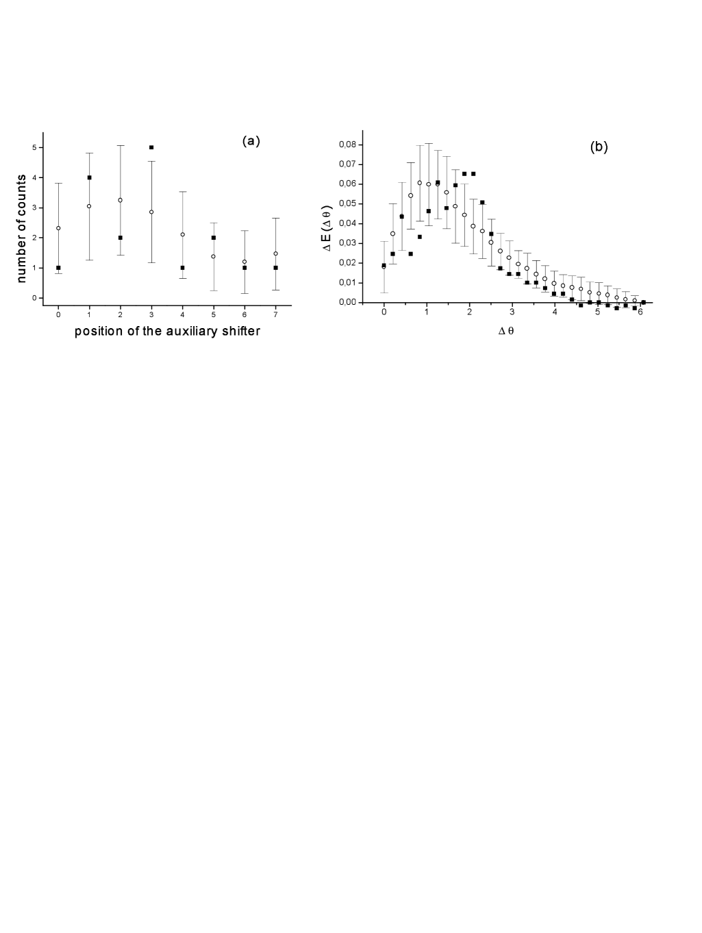
Figure 2: (a)Detected interference fringe $\bar{I}^{o}_{j}$ as mean of $690$ single measurements ($\circ$) and $68.3\%$ error bars for numerical values $I^{o}=2.21$ neutrons, $I^{h}=6.33$ neutrons, $I^{V}=1.03$ neutrons and $\theta=4.83$ rad. A typical single detection $I^{o}_{j}$ denoted by full squares is shown as an example. (b) Experimentally obtained $\Delta E(\Delta\theta)$ denoted by full squares are compared with theoretical prediction denoted by corresponding mean values ($\circ$) and error bars for $690$ samples.

Similarly to the previous case of strong field, where both methods are equally good, in the low field limit both methods are equally bad. Similarly in the limit of low visibility $I^{V}\ll\mbox{min}\{I_{o},I_{h}\}$, the results obtained with the use of the true Poissonian statistics are virtually identical to those yielded by the DFT [18]. No difference between the wave and quantum approach can be observed here. The difference between the predictions for the quantum and wave phase estimation in a realistic experiment should become significant for visibility close to unity and average number of detected particle of order one.

4 Experiment

Our experiments were performed at the neutron interferometry setup at the 250 kW TRIGA reactor in Vienna. Thermal neutrons which are emitted from the moderator of the reactor behave like statistically independent particles. Therefore the correct description of the counting statistics of the input beam and both output beams is a Poissonian distribution [17]. Fig. 1 shows the experimental arrangement. The input beam is split by the perfect crystal interferometer into two partially coherent beams. One of the beams passes a phase plate (grey shaded region) which introduces an unknown phase shift which has to be estimated from the experimental data. Then both beams are passing an auxiliary phase shifter which modulates the output intensities at the detectors $o$ and $h$. At the two output ports BF3 gas detectors enable single neutron counting with nearly 100 per cent efficiency. The very low intensities at the outgoing beams (1 neutron per second) allow a comfortable electronical separation of the detector pulses. The mean number of collected neutrons is a linear function of the counting time which enables an adjustment of the desired intensities by proper selection of the counting time. In neutron interferometry an auxiliary phase shifter can be rotated in several discrete positions denoted by indices $j$ in the intensity equation. Unique phase estimation is achieved even when other parameters of the setup (e.g. the mean intensities, the visibility and the frequency of the oscillation pattern) are unknown. In our experiment 8 equidistant positions of the phase shifter were used for generation of the intensity modulation.

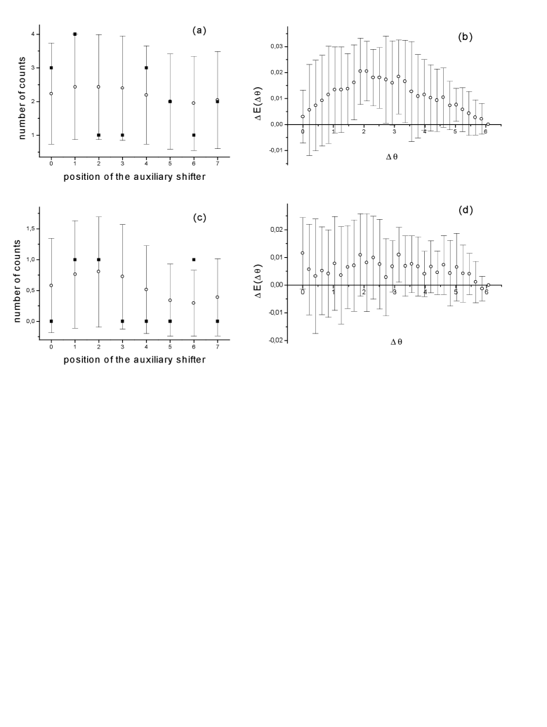
Figure 3: (a) Interference fringe $\bar{I}^{o}_{j}$ ($\circ$) and error bars corresponding to computer simulation of the experiment with numerical values $I^{o}=2.21$ neutrons, $I^{h}=6.33$ neutrons, $I^{V}=0.258$ neutrons and $\theta=4.83$ rad. A typical sample denoted by full squares is shown as an example. (b) $\Delta E(\Delta\theta)$ corresponding to the same computer simulation is evaluated. Mean values ($\circ$) and error bars corresponding to $690$ samples are given. The interpretation of panels (c) and (d) is the same as for (a) and (b), respectively. Numerical values are $I^{o}=0.551$ neutrons, $I^{h}=1.582$ neutrons, $I^{V}=0.258$ neutrons and $\theta=4.83$ rad.

To compare the efficiency of the NFM phase predictions with the optimum Poissonian MaxLik estimation the following procedure has been chosen. Each sample of data consisting of the number of neutrons counted in beams $o,h$ in eight positions $\Delta_{0},\ldots,\Delta_{7}$ (14), was processed using NFM formula (17) resulting in phase prediction $\theta_{N\!F\!M}$. The relative frequency $f_{g}(\Delta\theta)$ characterizes how many times the estimated phase $\theta_{N\!F\!M}$ falls into the chosen phase window $\Delta\theta$ (confidence interval) around the true phase shift. The same procedure was repeated for phase prediction based on numerical maximization of the Poissonian likelihood function (23) [9, 8] yielding the relative frequency of “hits” $f_{p}(\Delta\theta)$. The quantity

$$\Delta E(\Delta\theta) = f_{p}(\Delta\theta)-f_{g}(\Delta\theta)$$ (24)

represents the difference in efficiency of the quantum and wave phase estimations for the given phase window $\Delta\theta$. If this quantity is found to be positive, it means that the MaxLik estimation is better than its Gaussian counterpart (simply because more estimates of the phase shift fall into the chosen angular window if the former procedure is followed). If, on the other hand, this quantity is not different from zero (in a statistically significant way) the two data evaluation procedures are statistically equivalent and no discrimination is possible.

The result of the data analysis is shown in Figs. 2–4. Each figure consists of two different parts. The left panels show the detected (or simulated) data. The right panels then provide the interpretation of the corresponding data. Analysis of the experimental data is summarized in Fig. 2. In addition to experiment, two Monte–Carlo simulations have been performed simulating experimental conditions under which the difference between Poissonian and Gaussian predictions is negligible. The result of the simulations is shown in Fig. 3. Finally, the possibility to estimate several parameters simultaneously is illustrated in Fig. 4. The difference $\Delta E$ was calculated using $690$ experimental samples measured in experiment with average beam intensities $I^{o}$=2.2 neutrons, $I^{h}$=6.3 neutrons and visibility normalized with respect to $o$-beam being about $47\%$. As already explained in Section 2, this represents a critical situation, because even though there are less than $10$ counts in each experimental run, one is nonetheless trying to get an estimation of the value of the phase shift. The experimental values of $\Delta E$ are depicted in Fig. 2b by full squares. For comparison, a theoretical prediction corresponding to the same values of parameters as in the real experiment were simulated in the Monte–Carlo experiment using $40000$ samples. Open circles in the Fig. 2b show the corresponding mean values of the difference. However, since the experimental data are limited due to the experimental conditions and available time to the relatively small number of 690 samples, the real data are fluctuating around  the mean values. Statistical significance of the experimental results is demonstrated again using Monte–Carlo simulations. Other 20 simulations has been done, each of them with 690 samples The variance of the ensemble $\{\Delta E_{j}\},$ is shown in the Fig. 2b as “error bars” for each phase window.

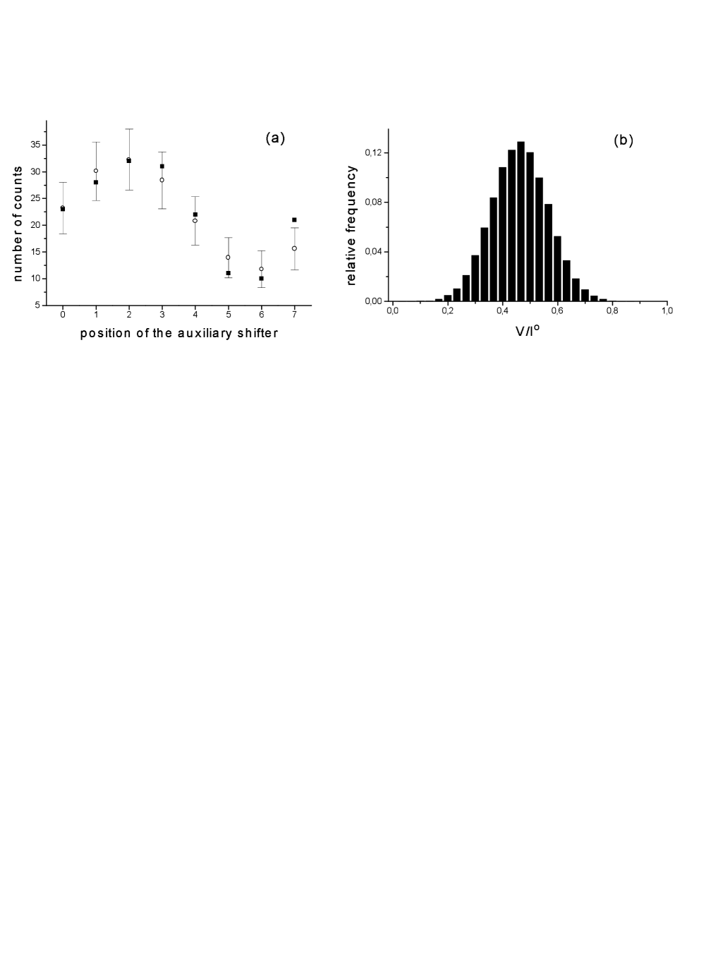
Figure 4: (a) Interference fringe $\bar{I}^{o}_{j}$ ($\circ$) and error bars corresponding to a computer simulation of the experiment with numerical values $I^{o}=22.1$ neutrons, $I^{h}=63.3$ neutrons, $I^{V}=10.3$ neutrons and $\theta=4.83$ rad. A typical sample is denoted by full squares as an example. (b) Histogram of estimated visibilities normalized with respect to $o$-beam obtained in the same simulation. The true normalized visibility is $46.7\%$.

A significant difference between the effectiveness of classical and optimum treatments is apparent in Fig. 2. The optimum estimation provides an improvement in fitting of the phase shift and the difference is beyond the estimation error, approximately 2.5 standard deviations in the optimum case. Obviously, no better performance of the MaxLik method can be expected for large values of the phase window $\Delta\theta$ (any sensible statistical method would yield rather reasonable results). Likewise, no real improvement over the Gaussian estimate can be expected when $\Delta\theta$ is close to zero, because too few data would then be accepted. The existence of a “best choice” for the phase window is therefore in itself an interesting feature of the method we propose. However notice that generalized NFM scheme (or equivalently DFT phase estimator) fits the phase shift quite well. The most pronounced difference is about $6\%$ in the window of width about $1.256$ rad. For example it means that the Gaussian fitting procedure hits this window $442$ times, whereas the Poissonian one $484$ times from a total number of $690$ events. The experimental difference in the score is therefore $42$ i.e. $6\%$ in favour of the latter method. This difference is a random number and theory predicts its value as $41\pm 12$. The observed difference is therefore not large, yet statistically significant.

In most cases, however, the difference between discrete and continuous nature of the signal is subtle enough to be hidden in various imperfections of the experimental setup. For illustration, a computer simulation of two experimental setups has been performed similarly to the above–mentioned case. A data analysis of the Monte-Carlo experiment with visibility as small as $1/4$ of the visibility in Fig. 2 is shown in Fig. 3b. No statistically significant discrimination between the Gaussian and Poissonian methods is possible in this case. The result of a simulation of an experiment with 4-times less energy of interfering beams is shown in Fig. 3d. Also in this case, no discrimination is possible. In spite of the apparent interference patterns the classical description of phase can be fully justified both in the cases of low visibility and low intensity. Particularly the latter case may appear as counterintuitive, since measurement with small number of particles is traditionally considered as a domain of quantum physics!

Unlike the case of phase, the MaxLik estimation of the visibility is strongly biased in the case of small intensities. There is simple explanation for this behaviour. In low-intensity regime the character of individual detected samples is determined rather by fluctuations then by actual parameters of the experimental setup as seen in Fig. 3c for example. The MaxLik estimation of the visibility fits this fluctuations and, as a consequence, the estimation is biased. This is particularly obvious in the case $I^{V}=0$, when interference pattern disappears, but MaxLik fitting yields a visibility of about $40\%$ due to fluctuations. Nevertheless, except the case of very low intensities, the estimated visibility is meaningful as demonstrated in Fig. 4, where a histogram of the estimated visibilities normalized with respect to $o$–beam is shown as result of a simulation with $10$ times stronger output beams compared to the output beams used in the experiment. It is apparent that the estimated visibilities are distributed with Gaussian–like shape around the value of the true visibility.

5 Conclusion

A statistically motivated analysis of neutron interferometry provides a correction to the previously introduced operational quantum phase concept. Since the standard approach has been universally derived, without considering the statistics of the interfering fields, it cannot be optimal. This additional knowledge may be used for improved predictions and testing. This scheme provides therefore a statistically motivated evaluation of the whole interferometric system. Instead of the question of the wave theory: “How precisely can the interference fringes be distinguished?” a more sophisticated question is here formulated as: “What statistical properties can be recognized from an interference pattern?” In particular, the experiment performed with neutrons demonstrated a measurable improvement of phase fitting for discrete Poissonian signals.

Acknowledgments

We acknowledge support by the TMR Network ERB FMRXCT 96-0057 ”Perfect Crystal Neutron Optics” of the European Union, by the grant No VS96028 of Czech Ministry of Education and by the East-West program of the Austrian Academy of Science.

References

- [1] A. Royer, Phys. Rev. A 53, 70 (1996).
- [2] D. T. Pegg, and S. M. Barnett, J. Mod. Opt. 44, 225 (1997).
- [3] V. Peřinová, A. Lukš, J. Peřina, Phase in Optics (World Scientific 1998, Singapore).
- [4] J. W. Noh, A. Fougères, and L. Mandel, Phys. Rev. A 45, 424 (1992).
- [5] J. W. Noh, A. Fougères, and L. Mandel, Phys. Rev. Lett. 71, 2579 (1993).
- [6] C. W. Helstrom, Quantum Detection and Estimation Theory (Academic Press 1976, New York).
- [7] K. R. W. Jones, Annals of Phys. 207, 140 (1991).
- [8] Z. Hradil, R. Myška, J. Peřina, M. Zawisky, Y. Hasegawa, and H. Rauch, Phys. Rev. Lett. 76, 4295 (1996).
- [9] M. Zawisky, Y. Hasegawa, H. Rauch, Z. Hradil, R. Myška and J. Peřina, J. Phys. A 31, 551 (1998).
- [10] A. S. Lane, S. L. Braunstein, and C. M. Caves, Phys. Rev. A 47, 1667 (1993).
- [11] Z. Hradil, Phys. Rev. A 55, R1561 (1997).
- [12] M. G. Kendall, A. Stuart, Advanced Theory of Statistics, vol.2 , Charles Griffin, London 1961.
- [13] Z. Hradil, Phys. Rev. A 47, 4532 (1993).
- [14] Th. Richter, Phys. Rev. A 56, 3134 (1997).
- [15] S. M. Barnett and D. T. Pegg, Phys. Rev. A 47, 4537 (1993).
- [16] J. R. Torgerson, L. Mandel, Phys. Rev. Lett. 76, 3939 (1996).
- [17] H. Rauch, J. Summhammer, M. Zawisky, E. Jericha, Phys. Rev. A 42 3726 (1990).
- [18] J. F. Walkup, J. W. Goodman, J. Opt. Soc. Am. 63, 399 (1973).