The Weyl representation on the torus

Centro Brasileiro de Pesquisas Físicas

Rua Xavier Sigaud 150, CEP 22290-180, RJ, Rio de Janeiro, Brazil

Abstract

We construct reflection and translation operators on the Hilbert space corresponding to the torus by projecting them from the plane. These operators are shown to have the same group properties as their analogue on the plane. The decomposition of operators in the basis of reflections corresponds to the Weyl or center representation, conjugate to the chord representation which is based on quantized translations. Thus, the symbol of any operator on the torus is derived as the projection of the symbol on the plane. The group properties allow us to derive the product law for an arbitrary number of operators in a simple form. The analogy between the center and the chord representations on the torus to those on the plane is then exploited to treat Hamiltonian systems defined on the torus and to formulate a path integral representation of the evolution operator. We derive its semiclassical approximation.

1 Introduction

The Weyl representation places quantum mechanics in phase space. The density operator is mapped into a real phase function that projects onto the position or momentum probability densities. The unitary operators corresponding to linear canonical transformations transform the Weyl symbol of any operator as a classical variable. Therefore, it is not surprising that the study of the semiclassical limit of nonintegrable systems has relied heavily on the Weyl representation as reviewed by reference [1].

The study of systems that are chaotic in the classical limit has developed several models supported by a compact phase space. The simplest choice is that of a $\left(2L\right)$-dimensional torus, corresponding to a system with $L$ degrees of freedom. Indeed, if the system propagates in discrete time ( a mapping of the torus onto itself) even the special case $L=1$ may be chaotic as is the case of the cat map [2], [3] or the baker’s map [4], [5]. It is well known that the Hilbert space corresponding to a classical torus is finite. We may picture the $N$ allowed positions and momenta as forming a lattice, the quantum phase space (QPS), even though no rigorous definition of position and momentum operators is available on the torus [6]. The semiclassical limit is then obtained as $N\sim\left(2\pi\hbar\right)^{-1}\rightarrow\infty.$

Though it is a great advantage to investigate numerically the propagation of finite vectors or matrices defined in the QPS, it is somewhat disconcerting that the difference between classical and quantum motion is more extreme on the torus than on the plane. This problem also manifests itself in the adaptation of the Weyl representation to the torus. The existing literature [7]-[10] relies mainly on formal procedures, so that the achievement of the classical limit as $N\rightarrow\infty$ may not be preceded by the emergence of classical structures even for finite $\hbar$, such as have been found for a plane phase space.

Clearly, a way to avoid this difficulty is to consider the classical torus as a periodic plane phase space, to quantize the latter and then to project this on QPS. We thus generalize the procedure of Hannay and Berry [3], allowing for arbitrary ”Bloch ” or ”Floquet ”angles for each circuit of the torus. It is then possible to project the appropriate plane translation and reflection operators onto the torus. Hence, we define the Weyl (or center) representation and its conjugate chord representation while maintaining the main geometrical features characteristic of the plane.

In section 2 we present the translation operators of momentum and position for a torus considered as the fundamental unit cell of the periodic plane. By also allowing tori made up of more than one cell, we show that the unit quantum torus may be obtained as the projection of the Hilbert space corresponding to such a larger torus. Finally, by connecting the Hilbert space for the plane to that of an infinitely large torus, we obtain the projection of plane operators onto the torus.

Section 3 summarizes important features of the Weyl representation on the plane. Defining the translation operators and their Fourier transform, the reflection operators, we derive the Weyl symbols and their product rules in terms of integrals over phase space polygons.

In section 4 we project appropriate translation operators onto QPS. However, it is found that the reflection operators are supported on a lattice with half the spacing of QPS . In consequence, the trace of these operators is not homogeneous, which leads to complications in the formulae for products of operators. Only in the case that $N$ is odd, can we simplify the product rule for the Weyl symbols into a form that is analogous to the theory in the plane. In any case, we need only half the number of sums derived in the previous work of Galleti and Toledo Pisa [8] and these sums depend on the symplectic areas of the same polygons arising in the plane theory. Finally, we discuss the restricted form of symplectic invariance that holds for the Weyl and chord representation on the torus: The Weyl symbols transform classically under the action of quantum cat maps.

Though we have motivated our paper through discrete time models, periodic Hamiltonians have obvious applications in solid state physics. Thus, section 5 is dedicated to the derivation of a path integral for the Weyl symbol of the propagator. This relies on the symplectic area of polygons as in the plane theory. In the semiclassical limit, the propagator is expressed in terms of the center generating function presented in reference [1].

Throughout this work we differentiate operators on the plane by italic $\widehat{A}$, as opposed to bold operators $\widehat{{\mathbf{A}}}$ on the torus.

2 Hilbert space for tori

Classical phase space of ($2L)$ dimensions may be considered to be periodic, so that we confer to it the topology of a $(2L)$ dimensional torus. Evidently, we may use invariance, with respect to symplectic transformations, to equate the periods $\Delta q=\Delta p=\nu$ of the position and momentum coordinates. The usual choice is $\nu=1$, but we will leave this as a free integer parameter so as to study the nesting of tori, that is, the case where quantization is imposed on a larger (periodic) region than the unit cell. Thus, the number of unit cells will be $\nu^{2L}.$

It is important to treat the specification of the Hilbert space of quantum states for the torus, or prequantization, independently from the dynamics of the system. That is, we treat the quantum kinematics, corresponding to the geometrical description of phase space at the classical level. A complete description for prequantization must include boundary conditions; which are here that the wave functions satisfy Bloch conditions:

$${\mathbf{\Psi}}(q+\nu) = e^{2\pi i\chi_{p}}{\mathbf{\Psi}}(q),$$ (2.1)

$${\mathbf{\tilde{}}{\Psi}}(p+\nu) = e^{-2\pi i\chi_{q}}{\mathbf{\tilde{}}{\Psi}}(p)$$ (2.2)

where

$${\mathbf{\tilde{}}{\Psi}}(p)=(2\pi\hbar)^{-1/2}\int e^{-ipq/\hbar}{\mathbf{\Psi}}(q)dq$$ (2.3)

and $2\pi i\chi_{p}$ and $2\pi i\chi_{q}$ are fixed arbitrary Floquet angles; that is, the prequantization depends on the vector $\chi=(\chi_{p},\chi_{q})$ whose coordinates are in the range $0\leq\chi_{q},\chi_{q}<1$.

It is a well known kinematical restriction [11] for torus quantization that there are

$$\nu^{2}N=\nu^{2}(2\pi\hbar)^{-1}$$ (2.4)

basis states for each degree of freedom, so that $N=(2\pi\hbar)^{-1}$ is the number of states corresponding to the unit cell .This is a crucial point: the compactness of the phase space implies in the finiteness of the dimension of the Hilbert space.

Recalling the translation operators $\widehat{T}_{p}=\exp\left(\frac{i\alpha}{\hbar}\widehat{q}\right)\,$ and $\widehat{T}_{q}=\exp\left(-\frac{i\beta}{\hbar}\widehat{p}\right)$ that respectively translates momentum by $\alpha$ and position by $\beta$ in the plane, we define minimal translators on the torus $\widehat{{\mathbf{T}}}_{p,\nu^{2}N}$ and $\widehat{{\mathbf{T}}}_{q,\nu^{2}N}$ with their discrete eigenstates $|{\mathbf{q}}_{n},\nu^{2}N>$ and $|{\mathbf{p}}_{m},\nu^{2}N>$ such that

$$\begin{array}[]{cc}\widehat{{\mathbf{T}}}_{p,\nu^{2}N}|{\mathbf{q}}_{n},\nu^{2}N>=e^{\left[\frac{2\pi i}{\nu^{2}N}(n+\chi_{q})\right]}|{\mathbf{q}}_{n},\nu^{2}N>&\widehat{{\mathbf{T}}}_{p,\nu^{2}N}|{\mathbf{p}}_{m},\nu^{2}N>=|{\mathbf{p}}_{m+1},\nu^{2}N>\\ \widehat{{\mathbf{T}}}_{q,\nu^{2}N}|{\mathbf{q}}_{n},\nu^{2}N>=|{\mathbf{q}}_{n+1},\nu^{2}N>&\widehat{{\mathbf{T}}}_{q,\nu^{2}N}|{\mathbf{p}}_{m},\nu^{2}N>=e^{\left[-\frac{2\pi i}{\nu^{2}N}(m+\chi_{p})\right]}|{\mathbf{p}}_{m},\nu^{2}N>\end{array}$$ (2.5)

The product of $\nu^{2}N$ translations on the basis states $|{\mathbf{q}}_{n},\nu^{2}N>$ or $|{\mathbf{p}}_{m},\nu^{2}N>\,$must return these to the same state, i.e. these Schwinger operators [12] satisfy

$$\left(\widehat{{\mathbf{T}}}_{p,\nu^{2}N}\right)^{\nu^{2}N}=e^{2\pi i\chi_{q}}\widehat{{\mathbf{1}}}_{\nu^{2}N}^{\chi}$$ (2.6)

and

$$\left(\widehat{{\mathbf{T}}}_{q,\nu^{2}N}\right)^{\nu^{2}N}=e^{-2\pi i\chi_{p}}\widehat{{\mathbf{1}}}_{\nu^{2}N}^{\chi}\ .$$ (2.7)

To define the Hilbert space ${\cal H}_{\nu^{2}N}^{\chi}$, we add the Hermitian structures

$$<{\mathbf{q}}_{n},\nu^{2}N|{\mathbf{q}}_{n^{\prime}},\nu^{2}N>=\delta_{n,n^{\prime}}^{(\nu^{2}N)}e^{\frac{2\pi i}{\nu^{2}N}(n-n^{\prime})\chi_{p}},$$ (2.8)

and

$$<{\mathbf{p}}_{m},\nu^{2}N|{\mathbf{p}}_{m^{\prime}},\nu^{2}N>=\delta_{m,m^{\prime}}^{(\nu^{2}N)}e^{-\frac{2\pi i}{\nu^{2}N}(m-m^{\prime})\chi_{q}}.$$ (2.9)

Here we define the $N$-periodic Kronecker delta

$$\delta_{m,n}^{(N)}\equiv\sum_{j=-\infty}^{\infty}\delta_{m,n+jN}.$$ (2.10)

The bases are exchanged with the transformation kernel

$$<{\mathbf{p}}_{m},\nu^{2}N|{\mathbf{q}}_{n},\nu^{2}N>=\frac{1}{\nu N^{1/2}}e^{2\pi i\frac{1}{\nu^{2}N}(m+\chi_{p})(n+\chi_{q})}\equiv F_{m,n},$$ (2.11)

forming a unitary matrix ( finite Fourier transformation).

Clearly, this last expression allows us to interpret the position ${\mathbf{q}}_{n}$ as corresponding to $q_{n}=\frac{1}{\nu N}(n+\chi_{q})$, whereas ${\mathbf{p}}_{m}$ corresponds to $p_{m}=\frac{1}{\nu N}(m+\chi_{p})$, leading to

$$<{\mathbf{p}}_{m},\nu^{2}N|{\mathbf{q}}_{n},\nu^{2}N>=(2\pi\hbar)^{-\frac{1}{2}}\exp\left(\frac{i}{\hbar}p_{m}q_{n}\right).$$ (2.12)

Likewise the $q$-Translator $\widehat{T}_{q}$, corresponds to a translation in the plane by $\Delta q=\frac{1}{\nu N}$ and the phase change $\exp\left[2\pi i\chi_{q}\right]$ results from the translation $\Delta q=\nu$  around the torus. Although the indices $n$ and $m$ can run over all integers, only $\nu^{2}N$ successive values will form a basis for the torus Hilbert space ${\cal H}_{\nu^{2}N}^{\chi}.$ We may keep to the fundamental range $\left[0,\nu^{2}N-1\right]$, corresponding to the square with side $\nu$, or extend to the periodic plane, by taking into account the phases $\chi$. These considerations apply to each of the $L$ degrees of freedom, so that in general the fundamental domain is a $\left(2L\right)$-hypercube. We see that position and momentum form a discrete web on the torus, as shown in Fig. 2.1, that we call the quantum phase space (QPS), following reference [8]:

$$x=\left(\begin{array}[]{c}p\\ q\end{array}\right)=\frac{1}{N}\left(\begin{array}[]{c}m+\chi_{p}\\ n+\chi_{q}\end{array}\right).$$ (2.13)

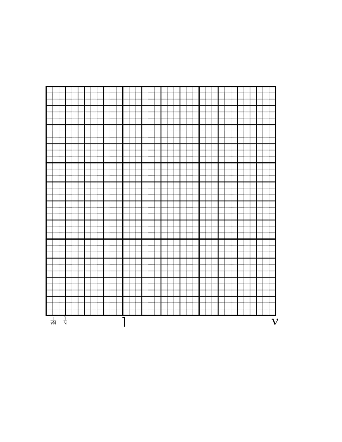
Figure 2.1: The quantum Phase space for $N=4$. The intersection of the bold lines in the unit square determine QPS for $\nu=1$, whereas the full figure corresponds to the choice $\nu=3$.

We now consider the relation between the Hilbert spaces of two nested tori ${\cal H}_{N}^{\chi}$ and ${\cal H}_{\nu^{2}N}^{\chi^{\prime}}$ with $\nu>1.$ The consideration for the QPS corresponding to ${\cal H}_{N}^{\chi}$ to be a sublattice of the QPS of ${\cal H}_{\nu^{2}N}^{\chi^{\prime}}$ is first that

$$\chi^{\prime}=\nu\chi-k,$$ (2.14)

where $k=(k_{p},k_{q})$ is an integer vector that denotes the number of loops around the torus made by $\chi$ when multiplied by $\nu.$ Thus $\chi^{\prime}$ is uniquely determined by $\chi.$ The indices for the larger Hilbert space ${\cal H}_{\nu^{2}N}^{\chi^{\prime}}$ for points in the fundamental domain of the smaller QPS are given by

$$m^{\prime} = \nu m+k_{p}$$ (2.15)

$$n^{\prime} = \nu n+k_{q}.$$ (2.16)

We can now define the Hilbert space ${\cal H}_{N}^{\chi}$ as a projection of the larger space ${\cal H}_{\nu^{2}N}^{\chi^{\prime}}.$ Indeed, it is easy to verify that if $|{\mathbf{q}}_{n^{\prime}},\nu^{2}N>$ are orthogonal position eigenstates for ${\cal H}_{\nu^{2}N}^{\chi^{\prime}}$, then

$$|{\mathbf{q}}_{n},N>_{\chi}=\frac{1}{\sqrt{\nu}}\sum_{r=0}^{\nu-1}e^{i2\pi\chi_{p}r}|{\mathbf{q}}_{\nu n+k}+r,\nu^{2}N>_{\chi^{\prime}}$$ (2.17)

form an appropriate orthonormal basis for ${\cal H}_{N}^{\chi}$. Thus, defining the projection operator

$$\widehat{{\mathbf{1}}}_{N}^{\chi}=\sum_{n=0}^{N-1}|{\mathbf{q}}_{n},N><{\mathbf{q}}_{n},N|$$ (2.18)

we verify that this is a Hermitian operator in ${\cal H}_{\nu^{2}N}^{\chi^{\prime}}$, and that

$$\widehat{{\mathbf{1}}}_{N}^{\chi}\widehat{{\mathbf{1}}}_{N}^{\chi}=\widehat{{\mathbf{1}}}_{N}^{\chi}.$$ (2.19)

Furthermore the states are obtained as

$$|{\mathbf{\Psi},}N>=\widehat{{\mathbf{1}}}_{N}^{\chi}{\mathbf{|}\Psi,}\nu^{2}N>.$$ (2.20)

For all operators $\widehat{{\mathbf{A}}}_{\nu^{2}N}$ acting in ${\cal H}_{\nu^{2}N}^{\chi^{\prime}},$ there is a projected operator which acts on ${\cal H}_{N}^{\chi}$:

$$\widehat{{\mathbf{A}}}_{N}=\widehat{{\mathbf{1}}}_{N}^{\chi}\widehat{{\mathbf{A}}}_{\nu^{2}N}\widehat{{\mathbf{1}}}_{N}^{\chi}.$$ (2.21)

If $\widehat{{\mathbf{A}}}_{\nu^{2}N}$ leaves ${\cal H}_{N}^{\chi}$ invariant, i.e. if

$$[\widehat{{\mathbf{1}}}_{N}^{\chi},\widehat{{\mathbf{A}}}_{\nu^{2}N}]=0,$$ (2.22)

then

$$\widehat{{\mathbf{A}}}_{N}=\widehat{{\mathbf{A}}}_{\nu^{2}N}\widehat{{\mathbf{1}}}_{N}^{\chi}.$$ (2.23)

We also verify that, for any pair of operators satisfying (2.22)

$$\widehat{{\mathbf{A}}}_{N}\widehat{{\mathbf{B}}}_{N}=\widehat{{\mathbf{A}}}_{\nu^{2}N}\widehat{{\mathbf{B}}}_{\nu^{2}N}\widehat{{\mathbf{1}}}_{N}^{\chi}.$$ (2.24)

In particular, we obtain the Schwinger translation operators for ${\cal H}_{N}^{\chi}$ as the projection of those in ${\cal H}_{\nu^{2}N}^{\chi^{\prime}}$:

$$\widehat{{\mathbf{T}}}_{q,N}=\widehat{{\mathbf{T}}}_{q,\nu^{2}N}\widehat{{\mathbf{1}}}_{N}^{\chi}\qquad;\qquad\widehat{{\mathbf{T}}}_{p,N}=\widehat{{\mathbf{T}}}_{p,\nu^{2}N}\widehat{{\mathbf{1}}}_{N}^{\chi}.$$ (2.25)

Let us now take the limit $\nu\rightarrow\infty$. Clearly, the variable $q_{n}$ becomes continuous in this limit as the volume of the torus $\nu^{2L}\rightarrow\infty$.Throughout the limit, the relation (2.14) defines an appropriate $\chi^{\prime}\left(\chi\right)$. The main step to recover the Banach space ${\cal H}_{{\mathbb{R}}}$ for the plane $\left(2L\right)$-dimensional phase space is to redefine the normalization so that

$$<q|q^{\prime}>=\delta(q-q^{\prime}),$$ (2.26)

introducing the Dirac delta function on the right, and the continuous Fourier integral for the change of basis:

$$<p|\psi>=\left(2\pi\hbar\right)^{-L/2}\int dq\exp\left(\frac{ipq}{\hbar}\right)<q|\psi>$$ (2.27)

In all other respects, the kinematics in the plane will coincide with that of an infinitely large torus. However, the normalization condition (2.26) implies a change in the way we express the sates in ${\cal H}_{N}^{\chi}$ in terms of those of ${\cal H}_{{\mathbb{R}}}$. For that purpose, we recall that for an unit torus

$$\sum_{r=0}^{N-1}e^{i\frac{2\pi}{N}(m-n)r}=N\delta_{m,n}^{(N)},$$ (2.28)

so we extend the definition of the $N$-periodic Kroeneker delta function to real numbers $x$ and $y$:

$$\delta_{x,y}^{(N)}\equiv\left\langle e^{i\frac{2\pi}{N}\left(x-y\right)k}\right\rangle_{k},$$ (2.29)

where $\left\langle...\right\rangle_{k}$ denotes the average over $k,$

$$\left\langle...\right\rangle_{k}=\lim_{r\rightarrow\infty}\frac{1}{r}\sum_{k=-\frac{r}{2}}^{\frac{r}{2}}.$$ (2.30)

From (2.29) we see that $\delta_{x,y}^{(N)}$ only depends on the difference $x-y$, so let us take $y=0$ for simplicity. For $x=r$ an integer number, the argument in (2.29) has period $N$. Then, the average is just (2.28) divided by $N,$ so the definition (2.29) is consistent with (2.10) for integer arguments. Let us now suppose $x=\frac{r}{d},$ a rational number. The argument in (2.29) thus has period $Nd$, so that

$$\delta_{x,0}^{(N)}=\frac{1}{Nd}\sum_{k=0}^{Nd-1}e^{i\frac{2\pi}{N}\frac{r}{d}k}=\frac{1}{Nd}\frac{1-e^{i2\pi r}}{1-e^{i\frac{2\pi}{Nd}r}}=\left\{\begin{array}[]{cc}1&\mbox{ if }r=0\qquad\mbox{mod}(Nd)\\ 0&\mbox{ otherwise}\end{array}\right..$$ (2.31)

Hence, once more the $N$-periodic Kroeneker delta function is different from zero only for $x$ being zero modulo $N$. By allowing $d\rightarrow\infty$ in (2.31) we can extend the definition of $\delta_{x,y}^{(N)}$ to irrational numbers, so that

$$\delta_{x,y}^{(N)}=\left\{\begin{array}[]{cc}1&\mbox{ only if }\left(x-y\right)=0\qquad\mbox{mod}(N)\\ 0&\mbox{ otherwise}\end{array}\right..$$ (2.32)

The definition (2.29) is an interpolation of (2.10), which will allows us to perform, not only sums with the $N$ periodic Kroeneker delta function, but also integrals. Indeed, we will relie on the formal equivalence:

$$\delta_{x,y}^{(N)}=\left\langle\delta(\frac{x-y}{N}-k)\right\rangle_{k}.$$ (2.33)

This is a consequence of the definition(2.29) and the Poisson sum formula,

$$\sum_{t\in{\mathbb{Z}}}\delta(x-t)=\sum_{k\in{\mathbb{Z}}}e^{i2\pi kx}.$$ (2.34)

Indeed, from the definition (2.29) we have

$$\frac{1}{\nu}\sum_{k=-\frac{\nu}{2}}^{\frac{\nu}{2}}e^{i\frac{2\pi}{N}\left(x-y\right)k}=\frac{1}{\nu}\sum_{k=-\frac{\nu}{2}}^{\frac{\nu}{2}}\delta(\frac{x-y}{N}-k)+\frac{1}{\nu}R_{\nu}(x-y)$$ (2.35)

with

$$R_{\nu}(x-y)=\sum_{k=-\frac{\nu}{2}}^{\frac{\nu}{2}}e^{i\frac{2\pi}{N}\left(x-y\right)k}-\sum_{k=-\frac{\nu}{2}}^{\frac{\nu}{2}}\delta(\frac{x-y}{N}-k).$$ (2.36)

From the Poisson sum formula (2.34), we have that, $\lim_{\nu\rightarrow\infty}R_{\nu}(x-y)=0,$ upon an appropriate ordering of the limits $\nu\rightarrow\infty$ and the width of the delta function$\rightarrow 0$.A consequence of (2.33) is that, for any function $f(t),$

$$\left\langle\delta(\frac{x-y}{N}-t)f(t)\right\rangle_{t}=\delta_{x,y}^{(N)}\;f(\frac{x-y}{N}).$$ (2.37)

Changing the origin, so as to keep the unit torus at the center of the larger torus, (2.17) must be replaced by

$$|{\mathbf{q}}_{n},N>=\lim_{\nu\rightarrow\infty}\frac{1}{\nu}\sum_{r=-\frac{\nu}{2}}^{\frac{\nu}{2}}|\frac{n+\chi_{q}}{N}+r>e^{2\pi ir\chi_{p}}.$$ (2.38)

A straightforward calculation using (2.37) shows that the orthonormality conditions (2.8) are obtained for the states defined in (2.38) with the normalization (2.26). So we consider that the states and the operators in the unit torus are obtained from the plane by projections. Recalling the definition (2.30) of the average, (2.38) can be written as

$$|{\mathbf{q}}_{n},N>=\left\langle|\frac{n+\chi_{q}}{N}+r>e^{2\pi ir\chi_{p}}\right\rangle_{r}$$ (2.39)

and the projection operator $\widehat{{\mathbf{1}}}_{N}^{\chi}\,$ is then given by (2.18). In the case of $\chi=0\,$ we thus retrieve the definition of Hannay and Berry [3] for ${\cal H}_{N}^{0}$ as the average over a periodic array of Dirac delta distributions. We will now derive the Weyl representation on the torus by projecting the properties that have been well established in the plane.

3 The Weyl representation on the plane

We here summarize the results obtained for the plane in reference [1] that will be projected onto the torus in the following sections. We define the operator corresponding to a general translation in phase space by the $\left(2L\right)$-dimensional vector $\xi=(\xi_{p},\xi_{q})$ as

$$\hat{T}_{\xi}\equiv\exp\left(\frac{i}{\hbar}\xi\wedge\hat{x}\right)\equiv\exp\left[\frac{i}{\hbar}(\xi_{p}.\hat{q}-\xi_{q}.\hat{p})\right],$$ (3.1)

where naturally $\hat{x}=(\hat{p},\hat{q})$ and the symplectic product $\xi\wedge\eta$ is defined as

$$\xi\wedge\eta=({\mathfrak{J}}\xi).\eta$$ (3.2)

with

$${\mathfrak{J}}=\left[\begin{array}[]{c|c}0&-1\\ \hline\cr 1&0\end{array}\right].$$ (3.3)

$\hat{T}_{\xi}$ is also known as a Heisenberg operator. In the case where either $\xi_{p}$ or $\xi_{q}=0$, we obtain respectively the operators $\hat{T}_{q}$ or $\hat{T}_{p}$ mentioned in the preceding section.

Acting on the Banach space ${\cal{H}_{{\mathbb{R}}}}$ we have

$$\widehat{T}_{\xi}|q_{a}>=e^{\frac{i}{\hbar}\xi_{p}(q_{a}+\frac{\xi_{q}}{2})}|q_{a}+\xi_{q}>$$ (3.4)

and

$$\widehat{T}_{\xi}|p_{a}>=e^{-\frac{i}{\hbar}\xi_{q}(p_{a}+\frac{\xi_{p}}{2})}|p_{a}+\xi_{p}>.$$ (3.5)

The classical group property is maintained within a phase factor:

$$\hat{T}_{\xi_{2}}\hat{T}_{\xi_{1}}=\hat{T}_{\xi_{1}+\xi_{2}}\ \exp[\frac{-i}{2\hbar}\xi_{1}\wedge\xi_{2}]=\hat{T}_{\xi_{1}+\xi_{2}}\ \exp[\frac{-i}{\hbar}D_{3}(\xi_{1},\xi_{2})],$$ (3.6)

where $D_{3}$ is the symplectic area of the triangle determined by two of its sides. Evidently, the inverse of the unitary operator $\hat{T}_{\xi}^{-1}=\hat{T}_{\xi}^{{\dagger}}=\hat{T}_{-\xi}$ and we can generalize (3.6):

$$\widehat{T}_{\xi_{1}}...\widehat{T}_{\xi j}=\widehat{T}_{\xi_{1}+....+\xi_{j}}e^{\frac{i}{\hbar}D_{j+1}(\xi_{1},....\xi_{j})},$$ (3.7)

where $D_{j+1}(\xi_{1},....\xi_{j})$ denotes the symplectic area of the $\left(j+1\right)$ sided polygon formed by the chords, $(\xi_{1},....\xi_{j})$.

The operator corresponding to a phase space reflection about a point $x=(p,q)$ is [1]

$$\widehat{R}_{x}\equiv(4\pi\hbar)^{-L}\int d\xi\quad e^{\frac{i}{\hbar}x\wedge\xi}\widehat{T}_{\xi}.$$ (3.8)

This operator has the following properties [1] :

$$\widehat{T}_{\xi}=(\pi\hbar)^{-L}\int dx\quad e^{-\frac{i}{\hbar}x\wedge\xi}\widehat{R}_{x}\ ,$$ (3.9)

$$\widehat{R}_{x}\widehat{T}_{\xi}=\widehat{R}_{x-\xi/2}e^{-\frac{i}{\hbar}x\wedge\xi}\ ,$$ (3.10)

$$\widehat{T}_{\xi}\widehat{R}_{x}=\widehat{R}_{x+\xi/2}e^{-\frac{i}{\hbar}x\wedge\xi}\$$ (3.11)

and

$$\widehat{R}_{x_{1}}\widehat{R}_{x_{2}}=\widehat{T}_{2(x_{2}-x_{1})}e^{\frac{i}{\hbar}2x_{1}\wedge x_{2}},$$ (3.12)

so that

$$\widehat{R}_{x}\widehat{R}_{x}=\widehat{1}\ .$$ (3.13)

The trace of the translation is

$$Tr\hat{T}_{\xi} = \int<q|T_{\xi}|q>dq=(2\pi\hbar)^{L}\delta(\xi_{p})\delta(\xi_{q})$$ (3.14)

$$= (2\pi\hbar)^{L}\delta(\xi)\$$

and then taking the Fourier transform,

$$Tr\hat{I\!\!\!\!R}_{x}=Tr2^{L}\hat{R}_{x}=(2\pi\hbar)^{-L}\int d\xi\exp\left[\frac{i}{\hbar}\ x\wedge\xi\right]Tr\hat{T}_{\xi}=1\ ,$$ (3.15)

where it is now also convenient to define the exact Fourier transform $\hat{I\!\!\!\!R}_{x}$ of $\hat{T}_{\xi}$. We recall that the classical transformation $R_{x}$ has a single fixed point ($x$ itself), whereas $T_{\xi}$ has fixed points only if $\xi=0$, when all points are fixed. These results are in general agreement with our intuition as to the classical correspondence of the traces of unitary operators. i.e. that the trace is related to the classical fixed points.

The above properties allow any operator $\hat{A}$ to be expressed as a linear superposition of elementary translation operators:

$$\hat{A}=\int\frac{d\xi}{(2\pi\hbar)^{L}}\ A(\xi)\hat{T}_{\xi}\ .$$ (3.16)

The confirmation results from

$$Tr(\hat{T}_{-\xi}\hat{A})=A(\xi)\ ,$$ (3.17)

The analogy with the classical chord generating function for canonical transformations is discussed in [1]. We can equally represent any operator $\hat{A}$ as a superposition of reflections:

$$\hat{A}=\int\frac{dx}{(2\pi\hbar)^{L}}\ A(x)\hat{I\!\!\!\!R}_{x}=\int\frac{dx}{(\pi\hbar)^{L}}\ A(x)\hat{R}_{x}\ .$$ (3.18)

Again we obtain the expansion coefficient by calculating

$$Tr(\hat{I\!\!\!\!R}_{x}\hat{A})=A(x)\ .$$ (3.19)

Notice that comparison of (3.16) and (3.18) with (3.8) and (3.9) yields

$$R_{x}(\xi)=2^{-L}\exp\left[\frac{i}{\hbar}\ x\wedge\xi\right]\ \ \ \mbox{and}\ \ \ T_{\xi}(x)=\exp\left[-\frac{i}{\hbar}\ x\wedge\xi\right]\ .$$ (3.20)

In analogy with our previous result, we may refer to $A(x)$ as the center representation of the operator $\hat{A}$, but the historic term is the Weyl representation.

The product laws of center and chord representations are of fundamental interest. Starting with the chord representation, we have, for the product $\hat{A}_{n}\hat{A}_{n-1}\cdots\hat{A}_{1}$,

$$A_{n}.A_{n-1}\cdots A_{1}(\xi)=\left(\frac{1}{2\pi\hbar}\right)^{L(n-1)}\int d\xi_{n}\cdots d\xi_{1}A_{n}(\xi_{n})\cdots$$

$$A_{1}(\xi_{1})\delta(\xi_{1}+\cdots\xi_{n}-\xi)\exp\left[-\frac{i}{\hbar}D_{n+1}(\xi_{1},\cdots,\xi_{n})\right],$$ (3.21)

where we note that the Dirac $\delta$-function has reduced the $(n+2)$-sided polygon with symplectic area $D_{n+2}$ to an $(n+1)$-sided polygon, with $n$ free sides. Evidently, we can now use the $\delta$-function to remove one of the variables in the integral, but (3.21) is in its most symmetric form.

We shall also need integral formulae for the product of operators in the center representation. The result depends crucially on the parity of the number of operators[1], so we will start with the simplest case where $n=2$. Proceeding from the definition  (3.18), we obtain

$$A_{2}.A_{1}(x)=\left(\frac{1}{\pi\hbar}\right)^{2L}\int dx_{2}dx_{1}A_{2}(x_{2})A_{1}(x_{1})\exp\left[\frac{i}{\hbar}\Delta_{3}(x,x_{1},x_{2})\right].$$ (3.22)

where $\Delta_{3}(x,x_{1},x_{2})=2(x_{1}\wedge x_{2}+x_{2}\wedge x+x\wedge x_{1})$ is the symplectic area of the triangle whose midpoints are, $x,x_{1},x_{2}$.

The extension to $(2n)$ operators is [1]

$$A_{2n}\cdots A_{1}(x)=$$

$$\left(\frac{1}{\pi\hbar}\right)^{2nL}\int dx_{2n}\cdots dx_{1}A_{2n}(x_{2n})\cdots A_{1}(x_{1})\exp\left\{\frac{i}{\hbar}\Delta_{2n+1}(x,x_{1},\cdots,x_{2n})\right\}.$$ (3.23)

Here the symplectic area $\Delta_{2n+1}$ corresponds to the $(2n+1)$-sided polygon circumscribed around the centers $(x,x_{1},\cdots,x_{2n})$.

The main advantage of the chord and center representation is their symplectic invariance. It is well known that linear classical canonical transformations $x^{\prime}=Mx$ correspond to unitary transformations in ${\cal{H}_{{\mathbb{R}}}}$

$$\widehat{A}\rightarrow\widehat{U}_{M}\widehat{A}\widehat{U}_{M}^{-1}.$$ (3.24)

The effect of such a unitary transformation on the chord and center representation is merely

$$A(x)\rightarrow A(Mx)\quad\mbox{and}\quad A(\xi)\rightarrow A(M\xi).$$ (3.25)

4 Weyl representation in the torus

4.1 Translation and Reflection Operators on the torus

In this section we will project the translations $\widehat{T}_{\xi}$ and reflections $\widehat{R}_{x}$ operators defined on ${\cal H}_{{\mathbb{R}}}$ onto the Hilbert space ${\cal H}_{N}^{\chi}$. Again we will treat the case of one degree of freedom explicitly, since the generalization is obvious. For this purpose we first investigate the action of the translation operators $\widehat{T}_{\xi}$ on the $|{\mathbf{q}}_{n},N>$ basis vectors defined by (2.39). From the effect of a translation (3.4) on a single position in the plane, we have

$$\widehat{T}_{\xi}|{\mathbf{q}}_{n},N>=\left\langle|\frac{n+\chi_{q}}{N}+k+\xi_{q}>e^{2\pi ik\chi_{p}}e^{\frac{i}{\hbar}\xi_{p}(\frac{n+\chi_{q}}{N}+k+\frac{1}{2}\xi_{q})}\right\rangle_{k},$$ (4.1)

using the relation (2.4) between $N$ and $\hbar$. This vector will belong to ${\cal H}_{N}^{\chi}$ only if it has the form (2.39), i.e., if we can write $\xi_{q}=\frac{s}{N}$ with $s$ an integer.

A similar treatment in the $|{\mathbf{p}}_{m},N>$ representation implies that

$$\widehat{T}_{\xi}|{\mathbf{p}}_{m},N>=\left\langle|\frac{m+\chi_{p}}{N}+k+\xi_{p}>e^{-2\pi ik\chi_{q}}e^{-\frac{i}{\hbar}\xi_{q}(\frac{m+\chi_{q}}{N}+k+\frac{\xi_{p}}{2})}\right\rangle_{k},$$ (4.2)

which does not belong to ${\cal H}_{N}^{\chi}$ unless we can write $\xi_{p}=\frac{r}{N}$ with $r$ an integer. So, as was already pointed in [11], the only translations that leave ${\cal H}_{N}^{\chi}$ invariant are those whose chords are $\xi=(\frac{r}{N},\frac{s}{N})$. For these cases we have

$$\widehat{T}_{\xi}|{\mathbf{q}}_{n},N > =\left\langle|\frac{n+\chi_{q}}{N}+k+\frac{s}{N}>e^{2\pi ik\chi_{p}}e^{i2\pi N\frac{r}{N}(\frac{n+\chi_{q}}{N}+k+\frac{s}{2N})}\right\rangle_{k}$$ (4.3)

$$= e^{\frac{i2\pi}{N}r(n+\frac{s}{2}+\chi_{q})}\left\langle|\frac{n+s+\chi_{q}}{N}+k>e^{2\pi ik(\chi_{p}+r)}\right\rangle_{k}$$

$$= e^{\frac{i2\pi}{N}r(n+\frac{s}{2}+\chi_{q})}|{\mathbf{q}}_{n+s},N>.$$

In short, we obtain the torus operator $\widehat{{\mathbf{T}}}_{\xi}^{\chi}$ in terms of the plane operator $\widehat{T}_{\xi}$ as

$$\widehat{{\mathbf{1}}}_{N}^{\chi}\widehat{T}_{\xi}\widehat{{\mathbf{1}}}_{N}^{\chi} = \left\{\begin{tabular}[]{lll}$\widehat{{\mathbf{T}}}_{\xi}^{\chi}$&$\mbox{if }$ $\xi=\left(\frac{r}{N},\frac{s}{N}\right),$where $r$ and $s$ are integers&\\ $0$&otherwise&\end{tabular}\right.$$ (4.6)

$$= \widehat{{\mathbf{T}}}_{\xi}^{\chi}\left\langle\delta\left(\xi-\frac{1}{N}\left(r,s\right)\right)\right\rangle_{\left(r,s\right)}=\widehat{T}_{\xi}\widehat{{\mathbf{1}}}_{N}^{\chi}\ ,$$ (4.7)

where the torus translation operators $\widehat{{\mathbf{T}}}_{\xi}^{\chi}\equiv\widehat{{\mathbf{T}}}_{r,s}^{\chi}$ are defined through

$$\widehat{{\mathbf{T}}}_{r,s}^{\chi}|{\mathbf{q}}_{n},N>=e^{i\frac{2\pi}{N}r(n+\chi_{q}+s/2)}|{\mathbf{q}}_{n+s},N>$$ (4.8)

and

$$\widehat{{\mathbf{T}}}_{r,s}^{\chi}|{\mathbf{p}}_{m},N>=e^{-i\frac{2\pi}{N}s(m+\chi_{p}+r/2)}|{\mathbf{p}}_{m+r},N>.$$ (4.9)

The last equality in (4.7) holds because $\widehat{T}_{\xi}$ and $\widehat{{\mathbf{1}}}_{N}^{\chi}$ commute for $\xi=\left(\frac{r}{N},\frac{s}{N}\right)$. We then see that the only translation operators that do not vanish on projection to the torus are those that leave ${\cal H}_{N}^{\chi}$ invariant. They correspond precisely to those classical transformations that preserve the QPS web. To simplify the notation, we will usually assume implicitly the $\chi$ dependence.

Let us now study some properties of the torus translation operators. For the case where the chords are the minimal translations in any one of the $q$ or $p$ directions, we recover the Schwinger operators [12] so that,

$$\widehat{{\mathbf{T}}}_{0,1}|{\mathbf{q}}_{n},N>\equiv\widehat{{\mathbf{T}}}_{q}|{\mathbf{q}}_{n},N>=|{\mathbf{q}}_{n+1},N>$$ (4.10)

and,

$$\widehat{{\mathbf{T}}}_{1,0}|{\mathbf{p}}_{m},N>\equiv\widehat{{\mathbf{T}}}_{p}|{\mathbf{p}}_{m},N>=|{\mathbf{p}}_{m+1},N>.$$ (4.11)

The kernel (2.11) implies that,

$$\widehat{{\mathbf{T}}}_{p}\widehat{{\mathbf{T}}}_{q}=e^{-\frac{2\pi i}{N}}\widehat{{\mathbf{T}}}_{q}\widehat{{\mathbf{T}}}_{p}.$$ (4.12)

so any translation operator in ${\cal H}_{N}^{\chi}$ is defined as

$$\widehat{{\mathbf{T}}}_{\xi}\equiv\widehat{{\mathbf{T}}}_{r,s}=e^{-\frac{i\pi rs}{N}}\widehat{{\mathbf{T}}}_{p}^{r}\widehat{{\mathbf{T}}}_{q}^{s}\ ,$$ (4.13)

with chords $\xi=(\frac{r}{N},\frac{s}{N}).$ We can express the matrix elements of the translation operators in the $|{\mathbf{q}}_{n},N>$ basis,

$$<{\mathbf{q}}_{m},N|\widehat{{\mathbf{T}}}_{r,s}|{\mathbf{q}}_{n},N>=e^{-i\frac{2\pi}{N}r(\frac{m+n}{2}+\chi_{q})}\delta_{m,n+s}^{(N)}e^{i\frac{2\pi}{N}(\frac{r}{2}+\chi_{p})(m-n-s)},$$ (4.14)

using the orthonormality relations of the states (2.8).The fact that the Hilbert space has finite dimension implies that linear operators acting on it will be represented by $N\times N$ matrices. Then $N^{2}$ linearly independent matrices will form a basis for the operators in ${\cal H}_{N}^{\chi}$. This is clear from the symmetries of the translation operators; through their action on ${\cal H}_{N}^{\chi}$ (4.8) we see that

$$\widehat{{\mathbf{T}}}_{\xi+{\mathbf{k}}}=(-1)^{sk_{p}-rk_{q}+k_{p}k_{q}N}e^{i2\pi(k_{p}\chi_{q}-k_{q}\chi_{p})}\widehat{{\mathbf{T}}}_{\xi}=e^{-i2\pi N\left[\left(\frac{\xi}{2}+\frac{\chi}{N}\right)\wedge{\mathbf{k}}+\frac{1}{4}{\mathbf{k}}\widetilde{{\mathfrak{J}}}{\mathbf{k}}\right]}\widehat{{\mathbf{T}}}_{\xi},$$ (4.15)

where ${\mathbf{k}}=(k_{p},k_{q})$ is a vector with integer components denoting chords that perform respectively $k_{p}$ and $k_{q}$ loops around the irreducible circuits of the torus. We have also defined the symmetric matrix

$$\widetilde{{\mathfrak{J}}}=\left[\begin{array}[]{c|c}0&1\\ \hline\cr 1&0\end{array}\right].$$ (4.16)

If we perform ${\mathbf{k}}$ loops around the torus, (4.15) implies that we recover the identity operator only up to a phase:

$$\widehat{{\mathbf{T}}}_{{\mathbf{k}}}=(-1)^{k_{p}k_{q}N}e^{i2\pi(k_{p}\chi_{q}-k_{q}\chi_{p})}\widehat{{\mathbf{1}}}_{N}^{\chi}.$$ (4.17)

Thus, to have a basis of operators we only need $r$ and $s$ in the range $[0,N-1]$, that is, we only need translations that perform less than one loop around the torus.

The second phase factor in expression (4.15) comes from the Bloch boundary conditions, but the $(-1)^{sk_{p}-rk_{q}+k_{p}k_{q}N}$ factor shows that we need two loops around the torus to recover the same operator, doubling the expected periodicity. This will have crucial importance in the construction of the reflection operators.

An important property of the translation operators, which can be deduced from (4.12) is

$$\widehat{{\mathbf{T}}}_{\xi_{2}}\widehat{{\mathbf{T}}}_{\xi_{1}}=\widehat{{\mathbf{T}}}_{\xi_{1}+\xi_{2}}e^{i\pi N\xi_{1}\wedge\xi_{2}},$$ (4.18)

which generalizes to

$$\widehat{{\mathbf{T}}}_{\xi_{1}}...\widehat{{\mathbf{T}}}_{\xi j}=\widehat{{\mathbf{T}}}_{\xi_{1}+....+\xi_{j}}e^{i\pi ND_{j+1}(\xi_{1},....\xi_{j})},$$ (4.19)

where $D_{j+1}(\xi_{1},....\xi_{j})$ denotes the area of $j+1$ sided polygon formed by the chords, $(\xi_{1},....\xi_{j})$, exactly as (3.7) in the plane case. From (4.18) and the unitarity of $\widehat{{\mathbf{T}}}_{\xi},$ we can see that

$$\widehat{{\mathbf{T}}}_{\xi}^{{\dagger}}=\widehat{{\mathbf{T}}}_{\xi}^{-1}=\widehat{{\mathbf{T}}}_{-\xi}.$$ (4.20)

Notice that (4.18) reduces to (4.12) for the particular case that $\xi_{1}$ and $\xi_{2}$ are vectors along the coordinate axis.

For the reflection operators, we use their definition (3.8) in terms of plane translations and then (4.7) projects the translations onto the torus, so that

$$\widehat{{\mathbf{R}}}_{x}^{\chi} = \widehat{{\mathbf{1}}}_{N}^{\chi}\widehat{R}_{x}\widehat{{\mathbf{1}}}_{N}^{\chi}=(4\pi\hbar)^{-L}\int d\xi\quad e^{\frac{i}{\hbar}x\wedge\xi}\widehat{{\mathbf{T}}}_{\xi}\left\langle\delta\left(\xi-\frac{{\mathbf{j}}}{N}\right)\right\rangle_{{\mathbf{j}}}$$ (4.21)

$$= (4\pi\hbar)^{-L}\left\langle e^{i2\pi x\wedge{\mathbf{j}}}\widehat{{\mathbf{T}}}_{\frac{{\mathbf{j}}}{N}}\right\rangle_{{\mathbf{j}}}.$$

To perform the average we use the periodicity of the torus translation (4.15), but we perform two loops around the torus, so that

$$\widehat{{\mathbf{R}}}_{x}^{\chi} = (4\pi\hbar)^{-L}\left(\frac{1}{2N}\right)^{2}\sum_{r=0}^{2N-1}\sum_{s=0}^{2N-1}\left\langle e^{-i2\pi N\left[\left(\frac{{\mathbf{j}}}{2N}+\frac{\chi}{N}\right)\wedge 2{\mathbf{k}}+{\mathbf{k}}\widetilde{{\mathfrak{J}}}{\mathbf{k}}\right]}e^{i2\pi x\wedge({\mathbf{j}+}2{\mathbf{k}}N{\mathbf{)}}}\widehat{{\mathbf{T}}}_{\frac{{\mathbf{j}}}{N}}\right\rangle_{{\mathbf{k}}}$$ (4.22)

$$= \frac{1}{2N}\sum_{r=0}^{2N-1}\sum_{s=0}^{2N-1}e^{-i2\pi x\wedge{\mathbf{j}}}\widehat{{\mathbf{T}}}_{\frac{{\mathbf{j}}}{N}}\left\langle e^{-i2\pi\left[\left(\chi-xN\right)\wedge 2{\mathbf{k}}\right]}\right\rangle_{{\mathbf{k}}}.$$

The ${\mathbf{k}}$ average is different from zero only if the point $x$ is such that $x=x_{a,b}\equiv\frac{1}{N}\left(\begin{array}[]{c}a+\chi_{p}\\ b+\chi_{q}\end{array}\right),\,$ with $a\,$ and $b$ half integers.

In short,

$$\widehat{{\mathbf{1}}}_{N}^{\chi}\widehat{R}_{x}\widehat{{\mathbf{1}}}_{N}^{\chi} = \left\{\begin{tabular}[]{lll}$\widehat{{\mathbf{R}}}_{x_{a,b}}^{\chi}$&$\mbox{if }$ $x=\left(\frac{a+\chi_{p}}{N},\frac{b+\chi_{q}}{N}\right),$ where $a$ and $b$ are half-integers&\\ $0$&otherwise&\end{tabular}\right.$$ (4.25)

$$= \widehat{{\mathbf{R}}}_{x_{a,b}}^{\chi}\left\langle\delta\left(x-\frac{{\mathbf{k}}}{2N}+\frac{\chi}{N}\right)\right\rangle_{{\mathbf{k}}}=\widehat{R}_{x}\widehat{{\mathbf{1}}}_{N}^{\chi},$$ (4.26)

where

$$\widehat{{\mathbf{R}}}_{x_{a,b}}^{\chi}=\frac{1}{2N}\sum_{r=0}^{2N-1}\sum_{s=0}^{2N-1}e^{i2\pi Nx\wedge\xi}\widehat{{\mathbf{T}}}_{\xi}^{\chi}$$ (4.27)

is the torus reflection on the center point $x_{a,b}$. The last equality in (4.26) holds because $\widehat{{\mathbf{R}}}_{x_{a,b}}^{\chi}$ commutes with $\widehat{{\mathbf{1}}}_{N}^{\chi}.$ Again, we will usually omit the explicit $\chi$ dependence.

The construction of the reflection operators on the torus replaces the Fourier transform (3.8) by a Fourier sum on the torus translation operators. The sums are to be taken over operators on one complete period; the symmetry properties (4.15) show that this period is obtained with chords that perform two loops around the torus, i.e. , the period is double that expected. So, although the basis of operators is formed with chords that perform up to one loop around the torus in the Fourier sum, we have to sum over chords that perform up to two loops. Thus, the basis operators are summed twice, but with different Fourier phases.

In what follows, the subscripts $(a,b)$ for the discrete centers and $(r,s)$ for the lattice of chords are implicit and they will be explicitly written only to avoid possible confusion. With the use of (2.28) we can derive the following extensively used relations,

$$\sum_{a=0}^{N-1/2}\sum_{b=0}^{N-1/2}e^{i2\pi Nx\wedge\xi}=(2N)^{2}\delta_{r,0}^{(2N)}\delta_{s,0}^{(2N)},$$ (4.28)

where all the sums over $a$ and $b$ are taken with step $\frac{1}{2}$, and

$$\sum_{r=0}^{2N-1}\sum_{s=0}^{2N-1}e^{i2\pi Nx\wedge\xi}=(2N)^{2}\delta_{b,0}^{(N)}\delta_{a,0}^{(N)}.$$ (4.29)

Here $\delta_{b,0}^{(2N)}$ is a period-$2N$ Kronecker delta function. Inserting (4.8) in (4.27)we find the action of the reflection operators on the Hilbert space:

$$\widehat{{\mathbf{R}}}_{x}|{\mathbf{q}}_{n},N>=e^{i\frac{2\pi}{N}2(b-n)(a+\chi_{p})}|{\mathbf{q}}_{2b-n},N>$$ (4.30)

and

$$\widehat{{\mathbf{R}}}_{x}|{\mathbf{p}}_{m},N>=e^{i\frac{2\pi}{N}2(a-m)(b+\chi_{q})}|{\mathbf{p}}_{2a-m},N>.$$ (4.31)

The unitarity of $\widehat{{\mathbf{R}}}_{x}$ is ensured by (4.30) and (4.31).

We then see that $\widehat{{\mathbf{R}}}_{x}$ reflects the (QPS) web about the point $x=(\frac{a+\chi_{p}}{N},\frac{b+\chi_{q}}{N})$. We need to include half-integer values of $a$ and $b$ so that with a given $|{\mathbf{q}}_{n},N>$ we can span all ${\cal H}_{N}^{\chi}$ by applying different $\widehat{{\mathbf{R}}}_{x}$. This is in complete agreement with the fact that the reflections that leave invariant the web formed by the QPS must include half-integer values of $a$ and $b$, conferring on these half-integers a clear geometrical meaning. So the centers of the reflections form a web whose spacing is half that of the QPS, as shown in Fig. 4.2. Once more, the only operators that do not vanish on projection to the torus are those that leave ${\cal H}_{N}^{\chi}$ invariant. These correspond classically to those transformations that leave the QPS web invariant.

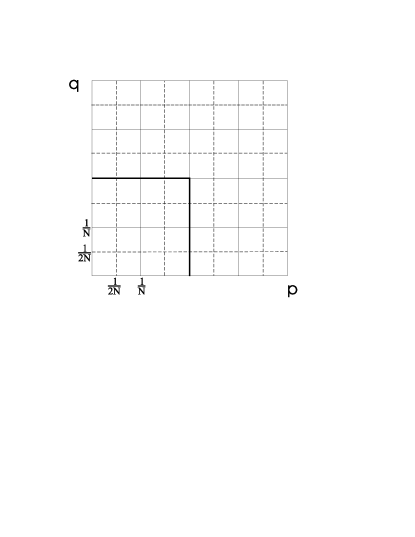
Figure 4.2: The quantum Phase space QPS for $N=4$ (solid line). The Weyl phase space WPS (doted line) is the grid of points $x$, centers of the reflection operators in QPS. The area in the bold square is the quarter-torus in which lie the centers $x,$ which label the basis of operators ${\mathbf{R}}_{x}$.

The matrix elements of the reflection operators in the $|{\mathbf{q}}_{n},N>$ basis are

$$<{\mathbf{q}}_{m},N|\widehat{{\mathbf{R}}}_{x}|{\mathbf{q}}_{n},N>=e^{i\frac{2\pi}{N}(m-n)(a+\chi_{q})}\delta_{m,2b-n}^{(N)}e^{i\frac{2\pi}{N}a(2b-n-m)}.$$ (4.32)

From (4.30) we can see the symmetry properties of these operators,

$$\widehat{{\mathbf{R}}}_{x+\frac{{\mathbf{k}}}{2}}=(-1)^{bk_{p}+ak_{q}+k_{p}k_{q}N}\widehat{{\mathbf{R}}}_{x}$$ (4.33)

where ${\mathbf{k}}=(k_{p},k_{q})$ is a vector with integer components. It is important to see that the domain of the variables $a$ and $b$ being integer and half-integer values, we have $(2N)^{2}$ different reflection operators in the unit square. But the symmetry properties (4.33) show that only $N^{2}$ of them are independent, so we take the values of $a$ and $b$ that belong to $[0,\frac{N-1}{2}]$ ; this forms a complete set of independent operators. That is, only one quarter of the torus is needed to define a complete set of reflection operators. The values of $x=(\frac{a+\chi_{p}}{N},\frac{b+\chi_{q}}{N})$ generated by these values of $a$ and $b$ do not all belong to the QPS; indeed we define here another space, the Weyl phase space, WPS, formed by the support of $x$ this is shown by the bold face area in Fig. 4.2. In the case where $N$ is odd, we will see later that WPS can be defined such that it coincides with the QPS.

By the use of (4.28) we can see that,

$$\widehat{{\mathbf{T}}}_{\xi}=\frac{1}{2N}\sum_{a=0}^{N-1/2}\sum_{b=0}^{N-1/2}e^{-i2\pi Nx\wedge\xi}\widehat{{\mathbf{R}}}_{x},$$ (4.34)

where we are again taking the sum with the indices running in an interval twice as large as that needed to define a basis of operators. This is so because (4.33) implies that classically equivalent reflections, through points diametrically opposed on any of the circuits of the torus, are only equal up to a phase.

We now investigate the group or cocycle properties of the translations and reflections defined in this section. It is important to note that the transformations treated here are such that they leave the web formed by the QPS invariant at the classical level, as well as the Hilbert space ${\cal H}_{N}^{\chi}$. With the help of (4.34) and (4.18), we obtain the following properties for these operators,

$$\widehat{{\mathbf{R}}}_{x}\widehat{{\mathbf{T}}}_{\xi}=\widehat{{\mathbf{R}}}_{x-\xi/2}e^{-i2\pi Nx\wedge\xi},$$ (4.35)

$$\widehat{{\mathbf{T}}}_{\xi}\widehat{{\mathbf{R}}}_{x}=\widehat{{\mathbf{R}}}_{x+\xi/2}e^{-i2\pi Nx\wedge\xi},$$ (4.36)

$$\widehat{{\mathbf{R}}}_{x_{1}}\widehat{{\mathbf{R}}}_{x_{2}}=\widehat{{\mathbf{T}}}_{2(x_{2}-x_{1})}e^{i2\pi N(2x_{1}\wedge x_{2})}.$$ (4.37)

We then have the same cocycle properties as in the plane: (3.6)-(3.12). This is a consequence of the commutation of operator products with projection (2.24) and will be of crucial importance when we derive the properties of the center and chord representations on the torus. Note that the characterization of the chords $\xi$ by integers and the centers $x$ by half-integers is respected by the group of operations above.

Another property which results from the last cocycle relation (4.37) is

$$\widehat{{\mathbf{R}}}_{x}\widehat{{\mathbf{R}}}_{x}=\widehat{{\mathbf{1}}}_{N}^{\chi},$$ (4.38)

in accordance with classical reflections. This means that

$$\widehat{{\mathbf{R}}}_{x}^{-1}=\widehat{{\mathbf{R}}}_{x}^{{\dagger}}=\widehat{{\mathbf{R}}}_{x},$$ (4.39)

that is, reflection operators on the torus are unitary and Hermitian.

It is important at this stage to examine the trace of these operators. Using (4.14) and (2.28), we have:

$${\mathbf{T}r}(\widehat{{\mathbf{T}}}_{\xi})=Ne^{i\frac{2\pi}{N}(\frac{rs}{2}+r\chi_{p}-s\chi_{p})}\delta_{r,0}^{(N)}\delta_{s,0}^{(N)}\equiv N\;e^{i\frac{2\pi}{N}(\frac{rs}{2}+r\chi_{q}-s\chi_{p})}\;\delta_{\xi}^{(N)}.$$ (4.40)

For the trace of the reflection operators, we recall (4.32), so

$$<{\mathbf{q}}_{n},N|\widehat{{\mathbf{R}}}_{x}|{\mathbf{q}}_{n},N>=\delta_{n,2b-n}^{(N)}e^{i\frac{2\pi}{N}a(2b-2n)}\ ,$$ (4.41)

which is different from zero only if

$$n=b\qquad\mbox{mod}\left(\frac{N}{2}\right).$$ (4.42)

However, if $b$ is half-integer and $N$ is even, for example, there would be no $n$ such that (4.42) is satisfied. In general we can have up to 2 solutions of (4.42) for $n\in\left[0,N-1\right]$, but they can have different phase contributions in (4.41). A careful inspection leads to:

$${\mathbf{T}r}(\widehat{{\mathbf{R}}}_{x}) = f_{N}(x)=\frac{1}{2}(1+(-1)^{2a}+(-1)^{2b}+(-1)^{2a+2b+N})=$$ (4.47)

$$= \left\{\begin{tabular}[]{ll}$0$&$\mbox{ if N is even and }a\mbox{ or }b\mbox{ semi-integers}$\\ $2$&$\mbox{ if N is even and }a\mbox{ and }b\mbox{ integers}$\\ $1$&$\mbox{if N is odd and }a\mbox{ or }b\mbox{ integers}$\\ $-1$&$\mbox{ if N is odd and }a\mbox{ and }b\mbox{ semi-integers}$\end{tabular}\right.$$

The importance of this result for the following theory calls for some intuitive explanation in terms of the reflections of the discrete periodic lattice. As in the plane case, we can relate ${\mathbf{T}r}(\widehat{{\mathbf{R}}}_{x})$ to the number of fixed points of the corresponding classical map. Indeed, for $N$ odd there is always a single fixed point, agreeing with the modulus of (4.47). If $N$ is even, there will only be fixed points if $x$ is characterized by integer numbers ($a,b$), in which case there are two.

4.2 Operators and their Symbols

Once we have defined the reflection and translation operators, we can decompose any operator as their linear combination. To construct the chord, or translation representation of an operator, we express any operator as a linear combination of translations. To have a complete basis, we need just $N^{2}$ operators, so that $r$ and $s$ run from $0$ to $N-1$. The chords $\xi=(\frac{r}{N},\frac{s}{N})$ having this property are said to belong to the fundamental domain. The other translation operators are obtained from these through the symmetry properties; that is, the fundamental translations are those which have chords smaller than one loop around any of the irreducible circuits of the torus in a given direction. The chord representation of an operator is defined as

$${\mathbf{A}}(\xi)\equiv{\mathbf{T}r}\left(\widehat{{\mathbf{A}}}\widehat{{\mathbf{T}}}_{-\xi}\right).$$ (4.48)

From the symbol, we recover the operator:

$$\widehat{{\mathbf{A}}}=\frac{1}{N}\sum_{r,s=0}^{N-1}{\mathbf{A}}(\xi)\widehat{{\mathbf{T}}}_{\xi}\equiv\frac{1}{N}\sum_{\xi}{\mathbf{A}}(\xi)\widehat{{\mathbf{T}}}_{\xi}.$$ (4.49)

Although, to recover the operator we only need the symbol defined in the fundamental domain (i.e. $r,s$ in $[0,N-1]$), (4.48) can be used to extend the definition of the symbol for $r$ and $s$ running among all integer numbers. Of course, these will not be independent of the symbols in the fundamental domain and, from the symmetry properties of $\widehat{{\mathbf{T}}}(\xi)$ (4.15), we see that ${\mathbf{A}}(\xi)$ satisfies

$${\mathbf{A}}(\xi+{\mathbf{k}})=(-1)^{sk_{p}+rk_{q}+k_{p}k_{q}N}e^{i2\pi(k_{p}\chi_{q}-k_{q}\chi_{p})}{\mathbf{A}}(\xi)=e^{-i2\pi N\left[\left(\frac{\xi}{2}+\frac{\chi}{N}\right)\wedge{\mathbf{k}}+\frac{1}{4}{\mathbf{k}}\widetilde{{\mathfrak{J}}}{\mathbf{k}}\right]}{\mathbf{A}}(\xi),$$ (4.50)

where ${\mathbf{k}}=(k_{p},k_{q})$ is a vector with integer components denoting chords that perform respectively $k_{p}$ and $k_{q}$ loops around the irreducible circuits of the torus. This is an important consequence of the fact that the symmetry properties of the symbol of operators are the same as those of the basis operators used to generate this symbol.

We now expand the operators in term of reflections; this is the center or Weyl representation. It is important to recall that we must take values of $a$ and $b$ that belong to $[0,\frac{N-1}{2}]$, that is, only one quarter of the torus is needed to define a complete set of reflection operators . The values of $x=(\frac{a+\chi_{p}}{N},\frac{b+\chi_{q}}{N})$ generated by these values of $a$ and $b$ define the Weyl phase space ,WPS, shown by the bold face area in Fig. 4.2.

We define the center symbol of an operator $\widehat{{\mathbf{A}}}$ such that,

$${\mathbf{A}}(x)\equiv{\mathbf{T}r}\left(\widehat{{\mathbf{A}}}\widehat{{\mathbf{R}}}_{x}\right).$$ (4.51)

From the symbol, we recover the operator through

$$\widehat{{\mathbf{A}}}=\frac{1}{N}\sum_{a,b=0}^{\frac{N-1}{2}}\widehat{{\mathbf{R}}}_{x}{\mathbf{A}}(x)\equiv\frac{1}{N}\sum_{x}\widehat{{\mathbf{R}}}_{x}{\mathbf{A}}(x).$$ (4.52)

The symmetry properties of $\widehat{{\mathbf{R}}}_{x}$ (4.33) imply

$${\mathbf{A}}(x+\frac{{\mathbf{k}}}{2})=(-1)^{bk_{p}+ak_{q}+k_{p}k_{q}N}{\mathbf{A}}(x),$$ (4.53)

for any vector ${\mathbf{k}}=(k_{p},k_{q})$ with integer components. This result had already been obtained by Hannay and Berry [3] for the Wigner function and we see here that it is general for any Weyl symbol on the torus.

As in the plane case, we derive some important properties of the translations and Weyl symbols. Notice first that:

$${\mathbf{R}}_{x}(\xi)={\mathbf{T}r}(\widehat{{\mathbf{R}}}_{x}\widehat{{\mathbf{T}}}_{-\xi})={\mathbf{T}r}(\widehat{{\mathbf{R}}}_{x+\xi/2})e^{i2\pi Nx\wedge\xi}=f_{N}(x+\xi/2)e^{i2\pi Nx\wedge\xi}$$ (4.54)

and

$${\mathbf{T}}_{\xi}(x)={\mathbf{T}r}(\widehat{{\mathbf{T}}}_{\xi}\widehat{{\mathbf{R}}}_{x})={\mathbf{T}r}(\widehat{{\mathbf{R}}}_{x+\xi/2})e^{-i2\pi Nx\wedge\xi}=f_{N}(x+\xi/2)e^{-i2\pi Nx\wedge\xi}.$$ (4.55)

The trace is now obtained as

$${\mathbf{T}r}\left(\widehat{{\mathbf{A}}}\right) = {\mathbf{A}}(\xi=0)$$ (4.56)

$$= \sum_{x}{\mathbf{A}}(x)f_{N}(x)=\frac{1}{2}\sum_{a,b=0}^{N-\frac{1}{2}}{\mathbf{A}}(x).$$ (4.57)

In the last equality we use the fact that the Weyl symbols for the entire torus are obtained from those of a quarter of it through the symmetry relations (4.53) and the definition of $f_{N}(x)$ (4.47).

The representation of the identity on the torus Hilbert space ${\cal H}_{N}^{\chi}$ has now the form:

$${\mathbf{1}}_{N}^{\chi}(x)=f_{N}(x)\ \ \ \mbox{ and }\ \ \ {\mathbf{1}}_{N}^{\chi}(\xi)=N\;\delta_{\xi}^{(N)}.$$ (4.58)

Hermitian operators are associated to the observables of the system and, in particular, the Hamiltonian generates the dynamics. Defined as $\widehat{{\mathbf{H}}}=\widehat{{\mathbf{H}}}^{{\dagger}}$, we obtain

$${\mathbf{H}}^{{\dagger}}(\xi)=[{\mathbf{H}}(-\xi)]^{*}\ \ \ \mbox{and}\ \ \ {\mathbf{H}}^{{\dagger}}(x)=[{\mathbf{H}}(x)]^{*}\ ,$$ (4.59)

just as for the plane case [1].

The role played in the plane case by the Fourier transform will be taken by the finite Fourier transform, since it allows us to exchange chords and centers as well as to change from center or chord to the position representation. But there are some small differences due to the $f_{N}(x)$ factors peculiar to the torus. Thus, in the exchange of centers and chords we have,

$${\mathbf{A}}(\xi) = {\mathbf{T}r}\left(\frac{1}{N}\sum_{x}\widehat{{\mathbf{R}}}_{x}{\mathbf{A}}(x)\widehat{{\mathbf{T}}}_{-\xi}\right)=\frac{1}{N}\sum_{x}{\mathbf{A}}(x){\mathbf{T}r}(\widehat{{\mathbf{R}}}_{x+\xi/2})e^{i2\pi Nx\wedge\xi}$$ (4.60)

$$= \frac{1}{N}\sum_{x}{\mathbf{A}}(x)f_{N}(x+\xi/2)e^{i2\pi Nx\wedge\xi},$$

whereas

$${\mathbf{A}}(x)=\frac{1}{N}\sum_{\xi}{\mathbf{A}}(\xi)f_{N}(x+\xi/2)e^{-i2\pi Nx\wedge\xi}.$$ (4.61)

Using (4.14) and (4.50) we obtain the position representation of an operator $\widehat{{\mathbf{A}}}$

$$<{\mathbf{q}}_{m},N|\widehat{{\mathbf{A}}}|{\mathbf{q}}_{n},N> = \frac{1}{N}\sum_{\xi}{\mathbf{A}}(\xi)<{\mathbf{q}}_{m},N|\widehat{{\mathbf{T}}}_{\xi}|{\mathbf{q}}_{n},N>$$ (4.62)

$$= \frac{1}{N}\sum_{r,s=0}^{N-1}{\mathbf{A}}(\xi_{r,s})e^{-i\frac{2\pi}{N}r(\frac{m+n}{2}+\chi_{q})}\delta_{m,n+s}^{(N)}e^{i\frac{2\pi}{N}(\frac{r}{2}+\chi_{p})(m-n-s)}$$

$$= \frac{1}{N}\sum_{r=0}^{N-1}{\mathbf{A}}(\xi_{r,m-n})e^{-i\frac{2\pi}{N}r(\frac{m+n}{2}+\chi_{q})}.$$

Note that in this last equation we are employing chords that may not belong to the fundamental domain; that is $m-n$ may not belong to $[0,N-1]$. However, the symbol for this chord is well defined through (4.48). If we restrict ourselves to chords that belong to the fundamental domain, we then have a supplementary $e^{i\frac{2\pi}{N}(\frac{r}{2}+\chi_{p})(m-n)}$ phase factor in the last sum. This kind of difficulty may appear in the following formulae, but, by allowing the indices to run over all integer numbers, the formulae become indeed much simpler, as is the case for (4.62).

Using the position representation

$$\widehat{{\mathbf{A}}}=\sum_{m,n=0}^{N-1}|{\mathbf{q}}_{m},N><{\mathbf{q}}_{m},N|\widehat{{\mathbf{A}}}|{\mathbf{q}}_{n},N><{\mathbf{q}}_{n},N|,$$ (4.63)

we retrieve the chord representation as

$${\mathbf{A}}(\xi) = {\mathbf{T}r}\left(\sum_{m,n=0}^{N-1}<{\mathbf{q}}_{m},N|\widehat{{\mathbf{A}}}|{\mathbf{q}}_{n},N>|{\mathbf{q}}_{m},N><{\mathbf{q}}_{n},N|\widehat{{\mathbf{T}}}_{-\xi}\right)$$ (4.64)

$$= \sum_{m,n=0}^{N-1}<{\mathbf{q}}_{m},N|\widehat{{\mathbf{A}}}|{\mathbf{q}}_{n},N>e^{-i\frac{2\pi}{N}r(\frac{m+n}{2}+\chi_{q})}\delta_{m,n+s}^{(N)}e^{i\frac{2\pi}{N}(\frac{r}{2}+\chi_{q})(m-n-s)}$$

$$= \sum_{n=0}^{N-1}<{\mathbf{q}}_{n+s},N|\widehat{{\mathbf{A}}}|{\mathbf{q}}_{n},N>e^{-i\frac{2\pi}{N}r(n+\frac{s}{2}+\chi_{q})}.$$

Using (4.32) and (4.53) we exchange the coordinate and the center representation:

$$<{\mathbf{q}}_{m},N|\widehat{{\mathbf{A}}}|{\mathbf{q}}_{n},N> = \frac{1}{N}\sum_{x}{\mathbf{A}}(x)<{\mathbf{q}}_{m},N|\widehat{{\mathbf{R}}}_{x}|{\mathbf{q}}_{n},N>$$ (4.65)

$$= \frac{1}{N}\sum_{a,b=0}^{\frac{N-1}{2}}{\mathbf{A}}(x_{a,b})e^{i\frac{2\pi}{N}2(b-n)(a+\chi_{p})}\delta_{m,2b-n}^{(N)}e^{i\frac{2\pi}{N}2\chi_{p}(m-2b+n)}$$

$$= \frac{1}{N}\sum_{a=0}^{\frac{N-1}{2}}{\mathbf{A}}(x_{a,\frac{m+n}{2}})e^{i\frac{2\pi}{N}(m-n)(a+\chi_{p})}.$$

Note that in this last formula we are taking the center point $x$ that does not belong to the fundamental domain (i.e. $\frac{m+n}{2}$ may not belong to $[0,\frac{N-1}{2}]$ ). We recover the center representation through

$${\mathbf{A}}(x) = {\mathbf{T}r}\left(\sum_{m,n=0}^{N-1}<{\mathbf{q}}_{m},N|\widehat{{\mathbf{A}}}|{\mathbf{q}}_{n},N>|{\mathbf{q}}_{m},N><{\mathbf{q}}_{n},N|\widehat{{\mathbf{R}}}_{x}\right)$$ (4.66)

$$= \sum_{m,n=0}^{N-1}<{\mathbf{q}}_{m},N|\widehat{{\mathbf{A}}}|{\mathbf{q}}_{n},N>e^{i\frac{2\pi}{N}(m-n)(a+\chi_{p})}\delta_{m,2b-n}^{(N)}e^{i\frac{2\pi}{N}a(2b-n-m)}$$

$$= \sum_{n=0}^{N-1}<{\mathbf{q}}_{2b-n},N|\widehat{{\mathbf{A}}}|{\mathbf{q}}_{n},N>e^{i\frac{2\pi}{N}2(b-n)(a+\chi_{p})}.$$

It would be possible to define the chord and the Weyl representations by equations (4.64) and (4.66) respectively. However, the geometrical structure, the role of the translations and reflection operators and the relation to the plane theory would then be relegated to curiosities.

4.3 Symbols of the product of operators

We now derive the product law of the symbols of the operators in these representations. Let us start with the chord representation (4.49). For this purpose we use ,(4.18) and (4.40) to obtain

$${\mathbf{A}B}(\xi) = {\mathbf{T}r}\left(\widehat{{\mathbf{A}}}\widehat{{\mathbf{B}}}\widehat{{\mathbf{T}}}_{-\xi}\right)=(\frac{1}{N})^{2}\sum_{\xi_{1},\xi_{2}}{\mathbf{A}}(\xi_{1}){\mathbf{B}}(\xi_{2}){\mathbf{T}r}\left(\widehat{{\mathbf{T}}}_{\xi_{1}}\widehat{{\mathbf{T}}}_{\xi_{2}}\widehat{{\mathbf{T}}}_{-\xi}\right)$$ (4.67)

$$= (\frac{1}{N})^{2}\sum_{\xi_{1},\xi_{2}}{\mathbf{A}}(\xi_{1}){\mathbf{B}}(\xi_{2})Ne^{i2\pi ND_{4}(\xi_{1},\xi_{2},-\xi)}{\mathbf{T}r}\left(\widehat{{\mathbf{T}}}_{\xi_{1}+\xi_{2}-\xi}\right)$$

$$= (\frac{1}{N})\sum_{\xi_{1}}{\mathbf{A}}(\xi_{1}){\mathbf{B}}(\xi-\xi_{1})e^{i2\pi ND_{3}(\xi_{1},-\xi)},$$

where we allow chords $\xi_{2}=\xi-\xi_{1}$ not to be in the fundamental domain. Let us now take the trace of the product; inserting (4.56) in (4.67) leads to

$${\mathbf{T}r}\left({\mathbf{A}B}\right)=(\frac{1}{N})\sum_{\xi_{1}}{\mathbf{A}}(\xi_{1}){\mathbf{B}}(-\xi_{1}).$$ (4.68)

The generalization of (4.67) for the product of an arbitrary number of operators is

$${\mathbf{A}}_{n}...{\mathbf{A}}_{1}(\xi) = (\frac{1}{N})^{n-1}\sum_{\xi_{1}...\xi_{n-1}}{\mathbf{A}}_{1}(\xi_{1})...$$ (4.69)

$$\!{\mathbf{A}}_{n-1}(\xi_{n-1}){\mathbf{A}}_{n}(\xi-\sum_{i=1}^{n-1}\xi_{i})\exp\left[-i2\pi ND_{n+1}(\xi_{1},...,\xi_{n-1},-\xi)\right].$$

Thus, the product rule for the chords is obtained from that in the plane by simply substituting the integral in (3.21) by the corresponding sum.

For the center symbol (4.51) the trace of the product is obtained using (4.37) and (4.40):

$${\mathbf{T}r}\left({\mathbf{A}B}\right) = (\frac{1}{N})^{2}\sum_{x_{1},x_{2}}{\mathbf{A}}(x_{2}){\mathbf{B}}(x_{1}){\mathbf{T}r}\left(\widehat{{\mathbf{R}}}_{x_{2}}\widehat{{\mathbf{R}}}_{x_{1}}\right)$$ (4.70)

$$= (\frac{1}{N})^{2}\sum_{x_{1},x_{2}}{\mathbf{A}}(x_{2}){\mathbf{B}}(x_{1})e^{i2\pi N(2x_{1}\wedge x_{2})}{\mathbf{T}r}\left(\widehat{{\mathbf{T}}}_{2(x_{2}-x_{1})}\right)$$

$$= (\frac{1}{N})\sum_{x_{1}}{\mathbf{A}}(x_{1}){\mathbf{B}}(x_{1}).$$

We will now derive the full product properties in the center representation (4.52); with the help of the group properties (4.37), (4.35) and (4.47) we have

$${\mathbf{A}B}(x) = {\mathbf{T}r}\left(\widehat{{\mathbf{A}}}\widehat{{\mathbf{B}}}\widehat{{\mathbf{R}}}_{x}\right)=(\frac{1}{N})^{2}\sum_{x_{1},x_{2}}{\mathbf{A}}(x_{2}){\mathbf{B}}(x_{1}){\mathbf{T}r}\left(\widehat{{\mathbf{R}}}_{x_{2}}\widehat{{\mathbf{R}}}_{x_{1}}\widehat{{\mathbf{R}}}_{x}\right)$$ (4.71)

$$= (\frac{1}{N})^{2}\sum_{x_{1},x_{2}}{\mathbf{A}}(x_{2}){\mathbf{B}}(x_{1})e^{i2\pi N2(x_{1}\wedge x_{2}+x_{2}\wedge x+x\wedge x_{1})}{\mathbf{T}r}\left(\widehat{{\mathbf{R}}}_{x+x_{2}-x_{1}}\right)$$

$$= (\frac{1}{N})^{2}\sum_{x_{1},x_{2}}{\mathbf{A}}(x_{2}){\mathbf{B}}(x_{1})e^{i2\pi N\Delta_{3}(x,x_{1},x_{2})}f_{N}(x+x_{2}-x_{1}),$$

where the symplectic area of the triangle $\Delta_{3}(x,x_{1},x_{2})$ was defined in section 3. Note that the sides of these triangles must be integer vectors in this case, because the symmetry of each side about its center implies that all the corners will be of the same type regardless of whether either $a$ or $b$ are integer or half-integer. The argument of the function $f_{N}$ defined in (4.47) can thus be any corner of the triangle as shown in Fig. 4.3(a). We thus find that the reflection properties of the QPS lead to a more complex product rule than for the plane (3.22).

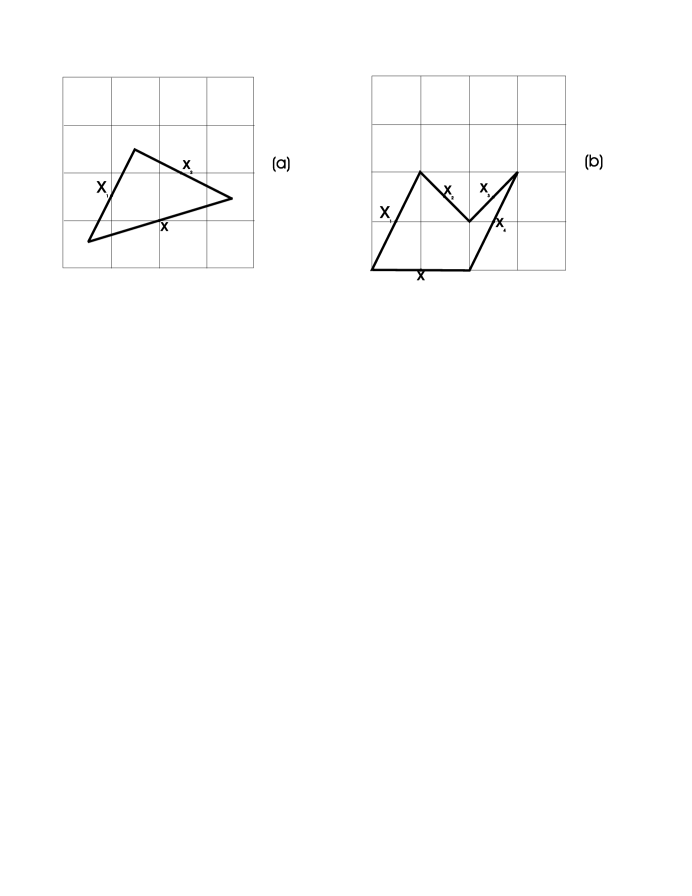
Figure 4.3: Two examples of polygons displaying the uniform nature of the vertices of the polygon. (a) all vertices lie on half integers: $f_{N}=0$ or $-1$ for $N$ respectively even or odd (b) the vertices lie on integers: $f_{N}=2$ or $1$ for $N$ respectively even or odd.

The generalization for the product of $2n$ operators is

$${\mathbf{A}}_{2n}...{\mathbf{A}}_{1}(x)=(\frac{1}{N})^{2n}\sum_{x_{1}...x_{2n}}{\mathbf{A}}_{2n}(x_{2n})$$

$${\mathbf{.}..A}_{1}(x_{1})e^{i2\pi N\Delta_{2n+1}(x,x_{2n},...,x_{1})}f_{N}(x+\sum_{j=1}^{2n}(-1)^{j}x_{j}),$$ (4.72)

where again the argument of $f_{N}$ is any corner of the polygon whose centers are $x,x_{2n},...,x_{1}$ (see an example in Fig. 4.3(b)). For an odd number of operators we just choose $\widehat{{\mathbf{A}}}_{1}=\widehat{{\mathbf{1}}}$, that is ${\mathbf{A}}_{1}(x_{1})=f_{N}(x_{1})$ in (4.72).

The product laws are the main result of this section. In contrast with the Weyl-like representation obtained by Galleti and Toledo Pisa [9], we only need half the number of sums (including the implicit sums in the trace of their formula (21)). Kaperskovitz and Peev [10] also have a Weyl-like representation, but only for the case of $N$ even. They perform products of 2 operators and the product law that they obtain is very similar to ours, although their result is not compatible with our geometrical interpretation, because we need half-integer vectors to completely describe the reflections of QPS. Most important is the fact that our formalism prescribes the product of an arbitrary even number of operators, just as for the plane, whereas previous results could only cope explicitly with the product of two operators at a time.

4.4 Weyl representation in QPS

If $N$ is odd, we can redefine the WPS so that it coincides with the QPS. For this purpose we define $X=(\frac{\alpha+\chi_{p}}{N},\frac{\beta+\chi_{q}}{N})$ so that ,

$$\alpha = a+j\frac{N}{2}\qquad\mbox{ where }j=\left\{\mbox{\begin{tabular}[]{ll}$0$&$\quad\mbox{ if }a\mbox{ is integer}$\\ $1$&$\quad\mbox{ otherwise}$\end{tabular} }\right.$$ (4.75)

$$\beta = b+k\frac{N}{2}\qquad\mbox{ where }k=\left\{\mbox{\begin{tabular}[]{ll}$0$&$\quad\mbox{ if }b\mbox{ is integer}$\\ $1$&$\quad\mbox{ otherwise}$\end{tabular} }\right.$$ (4.78)

We then have that $\alpha$ and $\beta$ are integers for the case were $N$ is odd. In other words for any $x$ there is a point $X$ such that

$$X=\frac{1}{N}\left(\begin{array}[]{c}\alpha\\ \beta\end{array}\right)+\frac{\chi}{N}=x+\frac{1}{2}{\mathbf{n}}$$ (4.79)

with ${\mathbf{n}}$ an integer vectors. If $N$ is even, the $\alpha$ and $\beta$ will have the same character ( integer or half-integer) as $a$ and $b$, so we cannot recover the QPS. In the rest of this section we will then restrict ourselves to the case where $N$ is odd. The symmetry relation (4.33) shows then that

$$\widehat{{\mathbf{R}}}_{X}=(-1)^{(2jb+2ja+jk)}\widehat{{\mathbf{R}}}_{x},$$ (4.80)

and with the use of (4.47) we have

$${\mathbf{T}r}(\widehat{{\mathbf{R}}}_{X})=1.$$ (4.81)

We now see that letting $a$ and $b$ run over the half-integers in $[0,\frac{N-1}{2}]$, we then have $\alpha$ and $\beta$ integers in $[0,N-1]$ and we recover the QPS. For this space we will now have a new Weyl representation

$${\mathbf{A}}(X)={\mathbf{T}r}\left(\widehat{{\mathbf{A}}}\widehat{{\mathbf{R}}}_{X}\right),$$ (4.82)

from which we recover the operator:

$$\widehat{{\mathbf{A}}}=\frac{1}{N}\sum_{\alpha,\beta=0}^{N-1}\widehat{{\mathbf{R}}}_{X}{\mathbf{A}}(X_{\alpha,\beta})\equiv\frac{1}{N}\sum_{X}\widehat{{\mathbf{R}}}_{X}{\mathbf{A}}(X).$$ (4.83)

We will now examine the properties of the product in this representation:

$${\mathbf{A}B}(X) = {\mathbf{T}r}\left(\widehat{{\mathbf{A}}}\widehat{{\mathbf{B}}}\widehat{{\mathbf{R}}}_{X_{\alpha,\beta}}\right)=(\frac{1}{N})^{2}\sum_{X_{1},X_{2}}{\mathbf{A}}(X_{2}){\mathbf{B}}(X_{1}){\mathbf{T}r}\left(\widehat{{\mathbf{R}}}_{X_{2}}\widehat{{\mathbf{R}}}_{X_{1}}\widehat{{\mathbf{R}}}_{X}\right)$$ (4.84)

$$(\frac{1}{N})^{2}\sum_{X_{1},X_{2}}{\mathbf{A}}(X_{2}){\mathbf{B}}(X_{1})e^{i2\pi N2(X_{1}\wedge X_{2}-X_{2}\wedge X+X\wedge X_{1})}{\mathbf{T}r}\left(\widehat{{\mathbf{R}}}_{X+X_{2}-X_{1}}\right)$$

$$(\frac{1}{N})^{2}\sum_{X_{1},X_{2}}{\mathbf{A}}(X_{2}){\mathbf{B}}(X_{1})e^{i2\pi N\Delta_{3}(X,X_{1},X_{2})}.$$

This last expression is very similar to the general case described in the previous section, but slightly simplified by the absence of the $f_{N}$ term, in close analogy to the plane formalism. For the product of $2n$ operators this generalizes to

$${\mathbf{A}}_{2n}...{\mathbf{A}}_{1}(X)=(\frac{1}{N})^{2n}\sum_{X_{1}...X_{2n}}{\mathbf{A}}_{2n}(X_{2n}){\mathbf{.}..A}_{1}(X_{1})e^{i2\pi N\Delta_{2n+1}(X,X_{2n,...},X_{1})}.$$ (4.85)

The absence of the $f_{N}$ factor in these simplified formulae may be understood from the fact that a polygon whose centers all lie on an integer lattice always has corners on the same lattice. Hence, $f_{N}$ is always unity for all corners if $N$ is odd.

In the same way, for $N$ odd, we can perform a transformation, similar to (4.79), to a set of chords $\tilde{\xi}$ that are even multiples of $\frac{1}{N}$. This set of chords will be complete if we now allow them to perform up to two loops around the circuits of the torus. This scheme can be generalized to perform quantization on centers or chords that are multiples of $\frac{\phi}{N}$ only if $2\phi$ and $N$ are coprime numbers. Then, the chord (or center) will be supported by a lattice of spacing $\frac{\phi}{N}$ and length $\phi$. This transformation will have importance for cat maps and will be studied in more details in reference [13].

4.5 Relation between symbols

There are many ways to represent a given operator $\widehat{A}$ that acts on the Banach space of the plane ${\cal H}_{{\mathbb{R}}}$. Among the different representations, the center and chord symbols are of special interest in this work. Projecting the operator $\widehat{A}$ onto the torus Hilbert space ${\cal H}_{N}^{\chi}$ through $\widehat{{\mathbf{A}}}=\widehat{{\mathbf{1}}}_{N}^{\chi}\widehat{A}\widehat{{\mathbf{1}}}_{N}^{\chi}$, it can be represented in terms of torus translations or reflections. We shall now show how the symbols on the torus can be obtained from their counterparts on the plane.

Starting with the chord representation, we calculate the torus symbol at points $\xi=\left(\frac{r}{N},\frac{s}{N}\right)$. From the fact that $\widehat{{\mathbf{T}}}_{-\xi}$ and $\widehat{{\mathbf{1}}}_{N}^{\chi}$ commute, we have

$${\mathbf{A}}(\xi)={\mathbf{T}r}\left(\widehat{{\mathbf{1}}}_{N}^{\chi}\widehat{A}\widehat{{\mathbf{1}}}_{N}^{\chi}\widehat{{\mathbf{T}}}_{-\xi}\right)={\mathbf{T}r}\left(\widehat{{\mathbf{1}}}_{N}^{\chi}\widehat{A}\widehat{T}_{-\xi}\widehat{{\mathbf{1}}}_{N}^{\chi}\right)={\mathbf{T}r}\left(\widehat{A}\widehat{T}_{-\xi}\widehat{{\mathbf{1}}}_{N}^{\chi}\right).$$ (4.86)

Then, we express the operator $\widehat{A}$ in terms of translations (3.17) and use the group properties of the translation operators (3.6) to obtain

$${\mathbf{A}}(\xi)=\int\frac{d\xi_{1}}{(2\pi\hbar)}\ A(\xi_{1})e^{\frac{i}{2\hbar}\xi_{1}\wedge\xi}{\mathbf{T}r}\left(\widehat{T}_{\xi_{1}-\xi}\widehat{{\mathbf{1}}}_{N}^{\chi}\right).$$ (4.87)

We now use the projection properties of the translation operators on the torus (4.7), so that

$${\mathbf{A}}(\xi)=\int\frac{d\xi_{1}}{(2\pi\hbar)}\ A(\xi_{1})e^{\frac{i}{2\hbar}\xi_{1}\wedge\xi}{\mathbf{T}r}\left(\widehat{{\mathbf{T}}}_{\xi_{1}-\xi}\right)\left\langle\delta\left(\xi_{1}-\xi-\frac{{\mathbf{k}}}{N}\right)\right\rangle_{{\mathbf{k}}}.$$ (4.88)

Performing the integral, with the help of the trace properties (4.40), we obtain

$${\mathbf{A}}(\xi) = \left\langle(-1)^{sk_{p}+rk_{q}+k_{p}k_{q}N}e^{i2\pi(k_{p}\chi_{q}-k_{q}\chi_{p})}A\left(\frac{r}{N}+k_{p},\frac{s}{N}+k_{q}\right)\right\rangle_{{\mathbf{k}}}=$$ (4.89)

$$\left\langle e^{i2\pi N\left[\left(\frac{\xi}{2}-\frac{\chi}{N}\right)\wedge{\mathbf{k}+}\frac{1}{4}{\mathbf{k}}\widetilde{{\mathfrak{J}}}{\mathbf{k}}\right]}A\left(\xi+{\mathbf{k}}\right)\right\rangle_{{\mathbf{k}}},$$

where the $(2L)$-dimensional vectors ${\mathbf{k}}$ have integer components. Note that we have to perform a phase weighted average on equivalent points to obtain the symbol on the torus. This is similar to the way Hannay and Berry quantize the cat map[3] in the coordinate representation.

We now proceed in a similar manner to derive the symbols in the center representation at the points $x=(\frac{a+\chi_{p}}{N},\frac{b+\chi_{q}}{N})$. Using the commutation of $\widehat{{\mathbf{R}}}_{x}$ with $\widehat{{\mathbf{1}}}_{N}^{\chi}$ and (3.17), we have

$${\mathbf{A}}(x)={\mathbf{T}r}\left(\widehat{{\mathbf{1}}}_{N}^{\chi}\widehat{A}\widehat{{\mathbf{R}}}_{x}\right)={\mathbf{T}r}\left(\widehat{{\mathbf{1}}}_{N}^{\chi}\int\frac{dy}{(\pi\hbar)}\ A(y)\hat{R}_{y}\widehat{R}_{x}\widehat{{\mathbf{1}}}_{N}^{\chi}\right),$$ (4.90)

which combined with the cocycle properties (3.12), becomes

$${\mathbf{A}}(x)={\mathbf{T}r}\left(\widehat{{\mathbf{1}}}_{N}^{\chi}\int\frac{dy}{(\pi\hbar)}\ A(y)e^{\frac{i}{\hbar}2y\wedge x}\widehat{T}_{2(x-y)}\widehat{{\mathbf{1}}}_{N}^{\chi}\right).$$ (4.91)

Projecting the translations on the torus (4.7), we have

$${\mathbf{A}}(x)=\int\frac{dy}{(\pi\hbar)}\ A(y)e^{\frac{i}{\hbar}2y\wedge x}{\mathbf{T}r}\left(\widehat{{\mathbf{T}}}_{2(x-y)}\right)\left\langle\delta\left(2(x-y)-\frac{{\mathbf{k}}}{N}\right)\right\rangle_{{\mathbf{k}}},$$ (4.92)

so that performing the integral we obtain,

$${\mathbf{A}}(x) = \left\langle e^{i2\pi(ak_{q}-bk_{p}+\frac{N}{2}k_{q}k_{p})}A\left(\frac{a+\chi_{p}}{N}+\frac{k_{p}}{2},\frac{b+\chi_{q}}{N}+\frac{k_{q}}{2}\right)\right\rangle_{{\mathbf{k}}}=$$ (4.93)

$$\left\langle e^{i2\pi N(\left[\left(x-\frac{\chi}{N}\right)\wedge{\mathbf{k}+}\frac{1}{4}{\mathbf{k}}\widetilde{{\mathfrak{J}}}{\mathbf{k}}\right])}A\left(x+\frac{{\mathbf{k}}}{2}\right)\right\rangle_{{\mathbf{k}}},$$

with the help of the trace properties (4.40).

We again have a phase weighted average on equivalent points, this is a general feature of any representation of projected operators ; only the phase will depend on the specific representation we are taking. An important feature of the center representation is that the phases do not have any dependence on the $\chi$ parameters of the quantization; this is best seen in (4.93). Note also that comparing (4.89) and (4.93) with (4.50) and (4.53) respectively, the phases are a consequence of the periodicity conditions of the symbols. It is important to note that if $\widehat{A}$ and $\widehat{{\mathbf{1}}}_{N}^{\chi}$ commute the restriction of $\widehat{A}$ on the Hilbert space ${\cal H}_{N}^{\chi}$ denotes an automorphism. Indeed, the commutation of $\widehat{A}$ and $\widehat{{\mathbf{1}}}_{N}^{\chi}$ implies that the symbols $A(x)$ and $A(\xi)$ are periodic functions. Otherwise the average defined in (4.89) and (4.93) may not exist, it may happen that the projected operator $\widehat{{\mathbf{A}}}=\widehat{{\mathbf{1}}}_{N}^{\chi}\widehat{A}\widehat{{\mathbf{1}}}_{N}^{\chi}=0.$

4.6 Symplectic invariance

At the end of section 3, we remarked that the center and the chord representations in the plane are invariant with respect to the quantum equivalents of linear canonical transformations, or symplectic transformations $x^{\prime}=Mx.$ The transformations for which the symplectic matrix $M$ is made up of integers are known colloquially as cat maps. These have the property that they leave invariant the unit torus. Because of the commutation of operator products with projection from the plane to the torus, the effect of a similarity transformation $\widehat{{\mathbf{A}}}\rightarrow\widehat{{\mathbf{U}}}_{M}\widehat{{\mathbf{A}}}\widehat{{\mathbf{U}}}_{M}^{-1}$ performed by a quantized cat map on any operator defined on the torus will be purely classical in the center or the chord representations:

$${\mathbf{A}}(x)\rightarrow{\mathbf{A}}(Mx)\quad\mbox{and\quad}{\mathbf{A}}(\xi)\rightarrow{\mathbf{A}}(M\xi).$$ (4.94)

Evidently, the matrix $M=1$ is a cat map; the product of cat maps is also a cat map, as is the inverse of a cat map. It follows that the set of all cat maps forms a subgroup of the symplectic transformations, which we will refer to as the feline group. Likewise, relations (4.94) indicate the feline invariance of the chord and center representations.

In a companion paper [13] we use the chord and center representations to study the properties of quantum cat maps of more than one degree of freedom. This extends previous work by Hannay and Berry [3] and Keating [14], [15] on two-dimensional cat maps. For completeness, we will just note that the symbol corresponding to $\widehat{{\mathbf{U}}}_{M}$ is

$${\mathbf{U}}_{M}(X)=\frac{1}{\sqrt{N^{L}}}\exp\left(\frac{i}{\hbar}XBX\right),$$ (4.95)

whereas the chord symbol is

$${\mathbf{U}}_{M}(\tilde{\xi})=\frac{1}{\sqrt{N^{L}}}\exp\left(-\frac{i}{\hbar}\tilde{\xi}\beta\tilde{\xi}\right).$$ (4.96)

For quantization performed on $\chi=0$, with $N$ an odd integer, $B$ and $\beta$ are integer symmetric matrices and the chords $\tilde{\xi}=\frac{2}{N}(r,s)$ (we perform quantization on a set of chords that are multiple of $\frac{2}{N}$). The symmetric matrices $B$ and $\beta$ in the above quadratic forms define the Cayley parametrization of the symplectic matrix $M:$

$$M=\frac{1-{\mathfrak{J}}B}{1+{\mathfrak{J}}B}=\frac{1+{\mathfrak{J}}\beta}{1-{\mathfrak{J}}\beta}.$$ (4.97)

In general, The Cayley matrices for a cat map may not be integer, leading to less transparent relation between the symplectic classical matrix $M$ and the symmetric matrices $B$ and $\beta$ in (4.95) and (4.96). They depend on Gaussian sums, as presented in reference [13].

5 Hamiltonians on the Torus and Path Integrals

We will now treat Hamiltonian systems on the torus. Let us first recall that the Poisson bracket relation that defines the symplectic product is the same for the torus as in the case of the plane. Therefore the classical generating function for canonical transformations are governed by the same composition laws as defined in [1] for the plane case. The only difference is that there would be different chords for a given center due to the periodic boundary conditions that identify centers with half the period as that of the whole torus.

We will then study dynamical systems with $L$ degrees of freedom for which there is defined a Hamiltonian function that generates the dynamics through Hamilton’s equations and that is periodic in all its $2L$ variables. For $L=1$ this kind of system has applications in solid state physics; it has been used to model electron eigenstates in a one-dimensional solid with an incommensurate modulation of the structure [16] and in models of Bloch electrons in a magnetic field [17]. It has also been shown [18] that this model presents a critical behavior giving rise to hierarchical structures in the solutions throughout the spectrum of the kind known as a Hofstadter butterfly [19] and to localization transitions from extended to localized states.

The Fourier theorem ensures that a classical Hamiltonian that is periodic in the plane can be written as

$$H(p,q)=\sum_{r,s=-\infty}^{+\infty}H_{r,s}e^{i2\pi(rp-sq)}.$$ (5.1)

To quantize this Hamiltonian, different ways may be taken involving different orderings. We choose the Weyl ordering, which is such that

$$\widehat{H}(\hat{p},\hat{q})=\sum_{r,s=-\infty}^{+\infty}H_{r,s}e^{i2\pi(r\hat{p}-s\hat{q})}.$$ (5.2)

With the definition of the translation operators on the plane (3.1), we immediately see that this is equivalent to

$$\widehat{H}(\hat{p},\hat{q})=\sum_{r,s=-\infty}^{+\infty}H_{r,s}\widehat{T}_{\xi_{r,s}}$$ (5.3)

where $\xi_{r,s}=(2\pi\hbar r,2\pi\hbar s)=(\frac{r}{N},\frac{s}{N})$. The Hamiltonian is then a linear combination of translation operators that leaves ${\cal H}_{N}^{\chi}$ invariant. If another ordering is chosen, there will be corrections to (5.3) of the order of $\frac{1}{N}$.

The quantal evolution of the system is determined by the propagator:

$$\widehat{U}_{t}=e^{\frac{i}{\hbar}t\widehat{H}}=\sum_{n=0}^{\infty}\frac{1}{n!}(\frac{i}{\hbar}t\widehat{H})^{n}.$$ (5.4)

This last relation implies that the propagator is a combination of products of torus translations in the expansion (5.3). These form a cocycle, as we already saw, so we can write

$$\widehat{U}_{t}=\sum_{r,s=-\infty}^{+\infty}U_{r,s}\widehat{T}_{\xi_{r,s}}.$$ (5.5)

Thus, the evolution operator also leaves ${\cal H}_{N}^{\chi}$ invariant. Written in this way we can see that the evolution operator and the Hamiltonian in the periodic plane have their chord representation in terms of torus translations only, in the form

$$U_{t}(\xi)=\sum_{r,s=-\infty}^{+\infty}U_{r,s}\delta(\xi_{r,s}-\xi).$$ (5.6)

Let us now project this operator on ${\cal H}_{N}^{\chi}$ and follow the evolution. We may first note that (2.24) and (5.3) allows us to write:

$$\widehat{{\mathbf{U}}}_{t} = \widehat{U}_{t}\widehat{{\mathbf{1}}}_{N}^{\chi}=\sum_{r,s=-\infty}^{+\infty}U_{r,s}\widehat{{\mathbf{T}}}_{\xi}=\sum_{n=0}^{\infty}\frac{1}{n!}(\frac{i}{\hbar}t\widehat{H})^{n}\widehat{{\mathbf{1}}}_{N}^{\chi}$$ (5.7)

$$= \sum_{n=0}^{\infty}\frac{1}{n!}(\frac{i}{\hbar}t\widehat{H}\widehat{{\mathbf{1}}}_{N}^{\chi})^{n}=e^{\frac{i}{\hbar}t{\mathbf{\hat{}}{H}}},$$

where ${\mathbf{\hat{}}{H}=}\widehat{{\mathbf{1}}}_{N}^{\chi}\hat{H}\widehat{{\mathbf{1}}}_{N}^{\chi}=\hat{H}\widehat{{\mathbf{1}}}_{N}^{\chi}$ is the Hamiltonian acting in the torus Hilbert space ${\cal H}_{N}^{\chi}.$

The unitarity evolution operators form a group, such that

$$\widehat{U}_{t}=(\widehat{U}_{\frac{t}{M}})^{M}.$$ (5.8)

Projecting onto the torus and using (2.24) we obtain

$$\widehat{{\mathbf{U}}}_{t} = \widehat{{\mathbf{1}}}_{N}^{\chi}\widehat{U}_{t}\widehat{{\mathbf{1}}}_{N}^{\chi}=\widehat{{\mathbf{1}}}_{N}^{\chi}(\widehat{U}_{\frac{t}{M}})^{M}\widehat{{\mathbf{1}}}_{N}^{\chi}$$ (5.9)

$$= (\widehat{{\mathbf{U}}}_{\frac{t}{M}})^{M}.$$ (5.10)

This last result is very important; the evolution and the projection commute.

We have two alternatives to obtain the center representation for (5.10) , i.e. to work from the plane relations or to work directly with the torus. First we note that (5.7) implies

$$\lim_{t\rightarrow 0}{\mathbf{U}}_{t}(x)=e^{\frac{i}{\hbar}t{\mathbf{H}}(x)}+0(t^{2}).$$ (5.11)

The use of (5.10) and (4.72) results in

$${\mathbf{U}}_{t}(x) = \lim_{M\rightarrow\infty}\left(\frac{1}{N}\right)^{2LM}\sum_{x_{i}=0}^{\frac{N-1}{2}}f_{N}(x+\sum_{j=1}^{2M}(-1)^{j}x_{j})$$ (5.12)

$$\exp\left\{\frac{i}{\hbar}\left[\,\Delta_{2M+1}(x,x_{1},...,x_{2M})-\frac{t}{2M}\sum_{i=1}^{2M}{\mathbf{H}(}x_{i})\right]\right\}.$$

For the odd $N$ case we obtain the representation on the points $X$ of QPS,

$${\mathbf{U}}_{t}(X)=\lim_{M\rightarrow\infty}\left(\frac{1}{N}\right)^{2LM}\sum_{X_{i}=0}^{N-1}\exp\left\{\frac{i}{\hbar}\left[\,\Delta_{2M+1}(X,X_{1},...,X_{2M})-\frac{t}{2M}\sum_{i=1}^{2M}{\mathbf{H}(}X_{i})\right]\right\}.$$ (5.13)

Notice that this expression for the projector relies on our original product rule for an arbitrary number of operators.

To take the projection, using (5.9), we can use the already known result about the propagator in the center representation on the plane [1], obtained as a path integral

$$U_{t}(x) = \lim_{M\rightarrow\infty}\int\frac{dx_{1}\cdots dx_{2M}}{(\pi\hbar)^{2ML}}\ \exp\left\{\frac{i}{\hbar}[\Delta_{2M+1}(x,x_{1},\cdots,x_{2M}))-\frac{t}{M}\sum_{n=1}^{2M}H(x_{n})]\right\}$$ (5.14)

$$= \int_{\gamma}{\cal D}_{\gamma}\,e^{i/\hbar S_{\gamma}(x)}.$$ (5.15)

Here we can see that for the odd $N$ case the propagator (5.13) is similar to (5.14) replacing the integral by the appropriate sums. The phase of the integral in (5.14) coincides with the center action $S_{\gamma}(x)$ for the polygonal path $\gamma$ with endpoints centered on $x$ and whose $k^{\prime}$th side is centered on $x_{k}$. The center variational principle ensures that this center action is stationary for the classical trajectories centered on $x$. In Fig. 5.4. we show two possible paths, whose actions are compared by the center variational principle.

Figure 5.4: Two possible paths, whose actions are compared by the center variational principle.

Now we project the symbol on the torus through (4.93). We then obtain

$${\mathbf{U}}_{t}(x) = \left(\frac{1}{2}\right)^{L}\left\langle e^{i2\pi N(\left[\left(x-\frac{\chi}{N}\right)\wedge{\mathbf{k}+}\frac{1}{4}{\mathbf{k}}\widetilde{{\mathfrak{J}}}{\mathbf{k}}\right])}\lim_{M\rightarrow\infty}\int\frac{dx_{1}\cdots dx_{2M}}{(\pi\hbar)^{2ML}}\right.$$ (5.16)

$$\left.\exp\left\{\frac{i}{\hbar}[\Delta_{2M+1}(x+\frac{k}{2},x_{1},\cdots,x_{2M}))-\frac{t}{2M}\sum_{n=1}^{2M}H(x_{n})]\right\}\right\rangle_{{\mathbf{k}}}$$

$$= \left(\frac{1}{2}\right)^{L}\left\langle e^{i2\pi N(\left[\left(x-\frac{\chi}{N}\right)\wedge{\mathbf{k}+}\frac{1}{4}{\mathbf{k}}\widetilde{{\mathfrak{J}}}{\mathbf{k}}\right])}\int_{\gamma}d\gamma\,\;e^{\frac{i}{\hbar}S_{\gamma}(x+\frac{{\mathbf{k}}}{2})}\right\rangle_{{\mathbf{k}}}.$$

Although it is not immediately evident, (5.12) and (5.16) are the same object; in (5.12), we first project on the torus and then perform the evolution, while in (5.16) we first evolve on the plane and the projection on the torus is performed later. But, since the projection (5.10) and evolution are commuting operations, (5.12) and (5.16) coincide. If we had defined the Weyl transformation intrinsically in the torus, without projecting from the plane, we could still derive a formula equivalent to (5.16) with the help of a Poisson transformation applied to (5.12).

To take the semiclassical limit, (5.16) is the adequate expression. Indeed, to apply this semiclassical limit we must evaluate the integrals in (5.14) by the stationary phase approximation as in [1], so

$$U_{t}(x)_{SC}\sim\sum_{j}2^{L}|\det(1+{\cal M}_{j})|^{-\frac{1}{2}}\ \exp\left\{i\hbar^{-1}S_{tj}(x)+i\mu_{j}\right\},$$ (5.17)

where ${\cal M}$ is the symplectic matrix for the linearized transformation between the neighborhood of the tips of the chord $\xi(x)$ generated by $S_{t}(x)$ as a center function.The index runs over all the contributing classical orbits. In the case of a single orbit, the corresponding Morse index $\mu_{j}=0$. Hence on the torus we obtain

$${\mathbf{U}}_{t}(x)_{SC} \sim \left\langle e^{i2\pi N(\left[\left(x-\frac{\chi}{N}\right)\wedge{\mathbf{k}+}\frac{1}{4}{\mathbf{k}}\widetilde{{\mathfrak{J}}}{\mathbf{k}}\right])}\right.$$ (5.18)

$$\left.\sum_{j}2^{L}|\det(1+{\cal M}_{j})|^{-\frac{1}{2}}\ \exp\left\{i\hbar^{-1}S_{tj}(x+\frac{k}{2})+i\gamma_{j}\right\}\right\rangle_{{\mathbf{k}}}.$$

The sum over $k$ is a sum over center points that are equivalent on the torus because of the boundary conditions, but are different points on the plane. To obtain the correct periodicity, the contribution of each term must be summed with different phases. But for each point there are several classical orbits whose chord is centered on it. The contribution of those orbits are obtained in the $j$ sum. Then, for the semiclassical propagator on the torus, we have a multiplicity of chords for any center point, due to the boundary conditions.

6 Conclusions

Our construction of the Weyl representation on the torus naturally generates the conjugate chord representation. This appears to be more useful on the torus than on the plane where it also arises. The advantage of our derivation of the Weyl representation resides in the clear geometrical interpretation of the operator basis in terms of translations and reflections in QPS, so that the law for the symbol of the product of operators acquires a simple form and generalizes to multiple products. It is important to note that the parity of the number of states $N$ plays an important role and the product law for $N$ odd is related to that in the plane case, by merely replacing the integrals by the appropriate sums.

Although the geometric interpretation is valid for toral geometries, the construction can be applied to any system whose Hilbert space has finite dimension irrespective of the geometric structure of the underlying phase space, except for its compactness. Indeed this operator basis and symbols can be applied, for example, to spin systems or many-body fermionic systems [20]. However, such a generalization destroys the intuitive interpretation of the semiclassical limit.

By defining the operators on the torus as the projections of their analogues on the plane, some important properties of the plane can then be used on the torus. We exploit this fact for periodic Hamiltonian systems where we map the continuous problem on a finite dimensional one. The path integral formulation of Hamiltonian systems on the plane allows us to obtain that on the torus, thus illuminating the semiclassical limit.

The symplectic invariance of the Weyl representation on the plane translates to the torus as the Feline invariance; this fact will be used to study cat maps of general dimension [13].

Acknowledgments: We thanks A. Voros, M. Saraceno and R.O. Vallejos for helpful discussions. We acknowledge financial support from Pronex-MCT and A.M.F.R. also thanks support from CLAF-CNPq.

References

- [1] A.M. Ozorio de Almeida, Physics Report 295 (1998), 266.
- [2] V.I. Arnold, ”Mathematical Methods of Classical Mechanics” (Springer, New York) (1978).
- [3] J.H. Hannay and M.V. Berry, Physica 1D (1980), 267-230.
- [4] M. L. Balazs and A. Voros, Annals of Physics 190 (1989), 1.
- [5] M. Saraceno, Annals of Physics 199 (1990), 37.
- [6] T.S. Santhanam and A.R. Tekumalla, Found. of Phys. 6 (1975), 5.
- [7] W.K. Wooters, Annals of Physics 176 (1987), 1.
- [8] D. Galetti and A.F.R. de Toledo Piza, Physica A 149 (1988), 267.
- [9] D. Galetti and A.F.R. de Toledo Piza, Physica A 186 (1992), 513.
- [10] W.K. Kaperskovitz and M. Peev, Annals of Physics 230 (1994), 21.
- [11] A.Bouzouina and S. De Bièvre, Commun. Math. Phys. 178 (1996), 83.
- [12] J. Schwinger, Proc. Nat. Acad. Sci. 46 (1960), 570 ,893,1401.
- [13] A.M.F. Rivas, A.M. Ozorio de Almeida and M. Saraceno, ”Quantization of Multidimensional Cat Maps” Preprint.
- [14] J. P. Keating, Nonlinearity 4 (1991), 277.
- [15] J. P. Keating, Nonlinearity 4 (1991), 309.
- [16] S. Aubry and G. André, Ann. Israel Phys. Soc. 3 (1979), 133-164.
- [17] P.G. Harper, Proc. Phys. Soc. A68 (1955), 874-892.
- [18] M. Wilkinson, Proc. R. Soc. London A 391 (1984), 305.
- [19] D. R. Hofstadter, Phys. Rev. B 14 (1976), 2239-2249.
- [20] D. Galetti and A.F.R. de Toledo Piza, Physica A 214 (1995), 207.