The second-order electron self-energy in hydrogen-like ions

Abstract

A calculation of the simplest part of the second-order electron self-energy (loop after loop irreducible contribution) for hydrogen-like ions with nuclear charge numbers $3\leq Z\leq 92$ is presented. This serves as a test for the more complicated second-order self-energy parts (loop inside loop and crossed loop contributions) for heavy one-electron ions. Our results are in strong disagreement with recent calculations of Mallampalli and Sapirstein for low $Z$ values but are compatible with the two known terms of the analytical $Z\alpha$-expansion.

The evaluation of the two-loop radiative corrections for hydrogen-like ions with arbitrary nuclear charge numbers $Z$ is a challenging theoretical problem important not only for comparison with experimental data for highly charged ions but also for obtaining reliable results in the low-$Z$ region. A general review of the present situation can be found in Ref. [1]. The only part of the two-loop corrections that remains uncalculated up to now is the second-order electron self-energy (SESE) part represented by the Feynman graphs in Fig. 1. The first diagram depicted in Fig. 1(a), i.e. the loop after loop irreducible contribution, was calculated for $Z=70,80,90,92$ [2] and recently for $1\leq Z\leq 92$ [3]. This correction is separately invariant under any covariant gauge transformation. The corresponding energy shift in Ref. [3] was called “perturbed orbital” contribution. The results in Refs. [2, 3] agree with each other.

The calculation of the remaining graphs depicted in Figs. 1(b)–(d) is a much more difficult problem. All these diagrams have to be evaluated together since only their sum is gauge invariant. Part of this sum was calculated recently for $Z=92$ with the use of the generalization of the potential expansion approach [4]. However, it is not clear whether this part is the major one of the total contribution or not.

Our final goal is also to calculate the remaining SESE corrections given by Figs. 1(b)–(d). We are planning to use the renormalization scheme developed in Ref. [5] (see also Ref. [6]) in combination with the partial-wave renormalization approach [7, 8]. Since the corresponding numerical calculations are extremely time-consuming (the same holds true for the calculations performed in Ref. [4]), we plan first to apply the approximate approach that works only for high $Z$ values and was applied recently for the first-order electron self-energy (SE) [9, 10]. This approach is based on the multiple commutator expansion method [11].

The original purpose of this work was to test this approximation also on the irreducible SESE correction. This means that we had first to calculate the SESE (a) contribution exactly and then to compare the result with the approximate one. We had also to elaborate the most time-saving procedure compatible with the level of accuracy sufficient for our purpose. Therefore we used the minimal number of grid points and partial waves that could guarantee the controlled accuracy within $10\%$. Working at this level of accuracy and using the exact expressions for SESE (a) we found that for the lower $Z$ values our results disagree very seriously (more than $50\%$ deviation) with the corresponding results in Ref. [3]. The comparison will be given below. This disagreement with previous calculations performed by Mallampalli and Sapirstein is a crucial point. In Ref. [3] the breakdown of the perturbation expansion in $Z\alpha$ was claimed even in the case for Hydrogen. However, perturbation theory has been employed intensively in many calculations of radiative effects and thus for the purpose of testing QED for weakly bound atomic electrons. Considerable success was made in this direction in last years [12, 13, 14]. In contrast to the results and the conclusions drawn in Ref. [3] our numerical results are consistent with the perturbation theory expansion for small $Z$. The fact that we can establish the validity of the $Z\alpha$ expansion in low-$Z$ region based on exact calculations represents the most important outcome of the present investigation.

The renomalized SE expression for the atomic state $|a\rangle$ is given by [9, 10]

$$\Delta E_{a} = \langle a|\hat{\Sigma}_{b}(E_{a})|a\rangle_{\rm ren}=\langle a|\hat{\Sigma}_{b}(E_{a})|a\rangle-\langle a|\hat{\Sigma}_{f}|a\rangle$$ (1)

$$= \sum_{l=0}^{\infty}\langle a|\hat{\Sigma}_{b}^{(l)}(E_{a})|a\rangle_{\rm ren}=\sum_{l=0}^{\infty}\left(\langle a|\hat{\Sigma}_{b}^{(l)}(E_{a})|a\rangle-\langle a|\hat{\Sigma}_{f}^{(l)}|a\rangle\right),$$ (2)

where $\hat{\Sigma}_{b}$ and $\hat{\Sigma}_{f}$ are the bound- and free-electron self-energy operators, and $\hat{\Sigma}_{b}^{(l)}$ and $\hat{\Sigma}_{f}^{(l)}$ are terms of the corresponding partial-wave expansions. The matrix element of $\hat{\Sigma}_{b}^{(l)}$ can be written as

$$\langle a|\hat{\Sigma}_{b}^{(l)}(E_{a})|a\rangle = \frac{\alpha}{\pi}(2l+1)\sum_{n}\Delta_{na}\ln{|\Delta_{na}|}$$ (3)

$$\times \langle a|\alpha_{1\mu}j_{l}(\Delta_{na}r_{1})\mathchoice{{\hbox{\boldmath$\displaystyle C$}}}{{\hbox{\boldmath$\textstyle C$}}}{{\hbox{\boldmath$\scriptstyle C$}}}{{\hbox{\boldmath$\scriptscriptstyle C$}}}^{l}_{1}|n\rangle\cdot\langle n|\alpha_{2}^{\mu}j_{l}(\Delta_{na}r_{2})\mathchoice{{\hbox{\boldmath$\displaystyle C$}}}{{\hbox{\boldmath$\textstyle C$}}}{{\hbox{\boldmath$\scriptstyle C$}}}{{\hbox{\boldmath$\scriptscriptstyle C$}}}^{l}_{2}|a\rangle$$ (4)

$$- \frac{\alpha}{2}(2l+1)\sum_{n}{\rm sgn}(E_{n})\Delta_{na}$$ (5)

$$\times \langle an|\alpha_{1\mu}\alpha_{2}^{\mu}j_{l}(\Delta_{na}r_{<})n_{l}(\Delta_{na}r_{>})\mathchoice{{\hbox{\boldmath$\displaystyle C$}}}{{\hbox{\boldmath$\textstyle C$}}}{{\hbox{\boldmath$\scriptstyle C$}}}{{\hbox{\boldmath$\scriptscriptstyle C$}}}^{l}_{1}\cdot\mathchoice{{\hbox{\boldmath$\displaystyle C$}}}{{\hbox{\boldmath$\textstyle C$}}}{{\hbox{\boldmath$\scriptstyle C$}}}{{\hbox{\boldmath$\scriptscriptstyle C$}}}^{l}_{2}|na\rangle,$$ (6)

where $\Delta_{na}=E_{n}-E_{a}$, $\alpha_{1\mu}\alpha_{2}^{\mu}=1-\mathchoice{{\hbox{\boldmath$\displaystyle\alpha$}}}{{\hbox{\boldmath$\textstyle\alpha$}}}{{\hbox{\boldmath$\scriptstyle\alpha$}}}{{\hbox{\boldmath$\scriptscriptstyle\alpha$}}}_{1}\cdot\mathchoice{{\hbox{\boldmath$\displaystyle\alpha$}}}{{\hbox{\boldmath$\textstyle\alpha$}}}{{\hbox{\boldmath$\scriptstyle\alpha$}}}{{\hbox{\boldmath$\scriptscriptstyle\alpha$}}}_{2}$, $j_{l}(z)$ and $n_{l}(z)$ are the spherical Bessel and Neumann functions, respectively, and $\mathchoice{{\hbox{\boldmath$\displaystyle C$}}}{{\hbox{\boldmath$\textstyle C$}}}{{\hbox{\boldmath$\scriptstyle C$}}}{{\hbox{\boldmath$\scriptscriptstyle C$}}}^{l}_{i}$ $(i=1,2)$ are the standard spherical tensors. We use here the relativistic units $\hbar=c=1$ with the fine-structure constant $\alpha$. The index $n$ runs over the whole spectrum of the Dirac equation for the bound electron.

The matrix elements $\langle a|\hat{\Sigma}_{f}^{(l)}|a\rangle$ that represent the mass-counterterms in the framework of the partial-wave renormalization approach [7, 8] read

$$\langle a|\hat{\Sigma}_{f}^{(l)}|a\rangle = \frac{\alpha}{\pi}(2l+1)\int{\rm d}\mathchoice{{\hbox{\boldmath$\displaystyle p$}}}{{\hbox{\boldmath$\textstyle p$}}}{{\hbox{\boldmath$\scriptstyle p$}}}{{\hbox{\boldmath$\scriptscriptstyle p$}}}\,|\langle\mathchoice{{\hbox{\boldmath$\displaystyle p$}}}{{\hbox{\boldmath$\textstyle p$}}}{{\hbox{\boldmath$\scriptstyle p$}}}{{\hbox{\boldmath$\scriptscriptstyle p$}}}|a\rangle|^{2}\int{\rm d}\mathchoice{{\hbox{\boldmath$\displaystyle q$}}}{{\hbox{\boldmath$\textstyle q$}}}{{\hbox{\boldmath$\scriptstyle q$}}}{{\hbox{\boldmath$\scriptscriptstyle q$}}}\,\Delta_{qp}\ln{|\Delta_{qp}|}$$ (7)

$$\times \langle\mathchoice{{\hbox{\boldmath$\displaystyle p$}}}{{\hbox{\boldmath$\textstyle p$}}}{{\hbox{\boldmath$\scriptstyle p$}}}{{\hbox{\boldmath$\scriptscriptstyle p$}}}|\alpha_{1\mu}j_{l}(\Delta_{qp}r_{1})\mathchoice{{\hbox{\boldmath$\displaystyle C$}}}{{\hbox{\boldmath$\textstyle C$}}}{{\hbox{\boldmath$\scriptstyle C$}}}{{\hbox{\boldmath$\scriptscriptstyle C$}}}^{l}_{1}|\mathchoice{{\hbox{\boldmath$\displaystyle q$}}}{{\hbox{\boldmath$\textstyle q$}}}{{\hbox{\boldmath$\scriptstyle q$}}}{{\hbox{\boldmath$\scriptscriptstyle q$}}}\rangle\cdot\langle\mathchoice{{\hbox{\boldmath$\displaystyle q$}}}{{\hbox{\boldmath$\textstyle q$}}}{{\hbox{\boldmath$\scriptstyle q$}}}{{\hbox{\boldmath$\scriptscriptstyle q$}}}|\alpha_{2}^{\mu}j_{l}(\Delta_{qp}r_{2})\mathchoice{{\hbox{\boldmath$\displaystyle C$}}}{{\hbox{\boldmath$\textstyle C$}}}{{\hbox{\boldmath$\scriptstyle C$}}}{{\hbox{\boldmath$\scriptscriptstyle C$}}}^{l}_{2}|\mathchoice{{\hbox{\boldmath$\displaystyle p$}}}{{\hbox{\boldmath$\textstyle p$}}}{{\hbox{\boldmath$\scriptstyle p$}}}{{\hbox{\boldmath$\scriptscriptstyle p$}}}\rangle$$ (8)

$$- \frac{\alpha}{2}(2l+1)\int{\rm d}\mathchoice{{\hbox{\boldmath$\displaystyle p$}}}{{\hbox{\boldmath$\textstyle p$}}}{{\hbox{\boldmath$\scriptstyle p$}}}{{\hbox{\boldmath$\scriptscriptstyle p$}}}\,|\langle\mathchoice{{\hbox{\boldmath$\displaystyle p$}}}{{\hbox{\boldmath$\textstyle p$}}}{{\hbox{\boldmath$\scriptstyle p$}}}{{\hbox{\boldmath$\scriptscriptstyle p$}}}|a\rangle|^{2}\int{\rm d}\mathchoice{{\hbox{\boldmath$\displaystyle q$}}}{{\hbox{\boldmath$\textstyle q$}}}{{\hbox{\boldmath$\scriptstyle q$}}}{{\hbox{\boldmath$\scriptscriptstyle q$}}}\,{\rm sgn}(E_{q})\Delta_{qp}$$ (9)

$$\times \langle\mathchoice{{\hbox{\boldmath$\displaystyle pq$}}}{{\hbox{\boldmath$\textstyle pq$}}}{{\hbox{\boldmath$\scriptstyle pq$}}}{{\hbox{\boldmath$\scriptscriptstyle pq$}}}|\alpha_{1\mu}\alpha_{2}^{\mu}j_{l}(\Delta_{qp}r_{<})n_{l}(\Delta_{qp}r_{>})\mathchoice{{\hbox{\boldmath$\displaystyle C$}}}{{\hbox{\boldmath$\textstyle C$}}}{{\hbox{\boldmath$\scriptstyle C$}}}{{\hbox{\boldmath$\scriptscriptstyle C$}}}^{l}_{1}\cdot\mathchoice{{\hbox{\boldmath$\displaystyle C$}}}{{\hbox{\boldmath$\textstyle C$}}}{{\hbox{\boldmath$\scriptstyle C$}}}{{\hbox{\boldmath$\scriptscriptstyle C$}}}^{l}_{2}|\mathchoice{{\hbox{\boldmath$\displaystyle qp$}}}{{\hbox{\boldmath$\textstyle qp$}}}{{\hbox{\boldmath$\scriptstyle qp$}}}{{\hbox{\boldmath$\scriptscriptstyle qp$}}}\rangle,$$ (10)

where $\Delta_{qp}=E_{q}-E_{p}$. By means of the symbols $|\mathchoice{{\hbox{\boldmath$\displaystyle p$}}}{{\hbox{\boldmath$\textstyle p$}}}{{\hbox{\boldmath$\scriptstyle p$}}}{{\hbox{\boldmath$\scriptscriptstyle p$}}}\rangle$ and $|\mathchoice{{\hbox{\boldmath$\displaystyle q$}}}{{\hbox{\boldmath$\textstyle q$}}}{{\hbox{\boldmath$\scriptstyle q$}}}{{\hbox{\boldmath$\scriptscriptstyle q$}}}\rangle$ we denote the spherical-wave solutions of the free-electron Dirac equation. Integration over $\textstyle p$ is interpreted as integration over the energies $E_{p}=\pm\sqrt{m_{e}^{2}+p^{2}}$, where $m_{e}$ is the electron mass and $p$ is the absolute value of the electron momentum. The summations over angular quantum numbers are also understood. The free-electron wave functions are normalized to $\delta$-function in the energy. Equations (2) – (10) are also valid for arbitrary electronic states $|a\rangle$ and for nondiagonal matrix elements of the type $\langle a|\hat{\Sigma}{(E_{a})}|n\rangle$ provided that $|a\rangle$ is the ground state.

The B-spline numerical approach [15] was used in Refs. [9, 10] to approximate the sums in Eq. (6) and the integrals over $\textstyle q$ and $\textstyle p$ in Eq. (10). The number of grid points was $N=140$, the order of splines $k=9$, and the number of partial waves $s=16$ [9]. The accuracy achieved in Ref. [9] compared to the exact Mohrs’ results for the point-like nucleus [16] was $0.1\%$ for $Z=10$ and $0.001\%$ for $Z=92$.

It was observed in Ref. [10] that the terms of Eqs. (2) – (10) containing $\ln|\Delta_{na}|$ are dominant for small $Z$ values and that the terms containing sgn$(E_{n})$ are dominant for large $Z$ values. From the results obtained in Ref. [9] we can deduce that logarithmic term gives $99\%$ of the total value for $Z=10$ and the sign term yields $95\%$ of the total value for $Z=92$. The terms analogous to the sign terms in SE can be also found in the expressions for SESE corrections. One can try to use the sign approximation for the estimate of the unknown parts of SESE for highly charged ions. In this work we will try to test this approximation on the SESE (a) correction that can be treated also without any approximations.

The expression for the SESE (a) correction can be written in the form [2, 3]

$$\Delta E_{a}^{\rm irr}=\sum_{l_{1},l_{2}=0}^{\infty}\sum_{n}{\!}^{{}^{\prime}}\frac{\langle a|\hat{\Sigma}_{b}^{(l_{1})}(E_{a})|n\rangle_{\rm ren}\langle n|\hat{\Sigma}_{b}^{(l_{2})}(E_{a})|a\rangle_{\rm ren}}{E_{a}-E_{n}},$$ (11)

where the summation over $n$ is extended over the whole Dirac spectrum for the bound electron and $E_{n}=E_{a}$ term is excluded. For evaluation of the matrix elements in the numerator of Eq. (11) the formulas (6) and (10) can be applied. Thus in total we have to perform 3-fold (or even 4-fold, for counterterms) summations over the spline Dirac spectrum.

The minimal set of parameters for the numerical spline calculations was chosen to be: $N=28$, $k=9$ and $s=7$, while in Ref. [3] $N=50$ and $12\leq s\leq 40$. However, this minimal set in our approach allowed us to keep the controlled accuracy better than $10\%$. As an example, the convergence of our method for the SE correction (2) in the ground state for $Z=10$ is demonstrated in Table I. Both of the partial-wave sequences for odd and even $l$ values have been assumed to converge to a common limit. The accuracy of the calculation is $7.8\%$ for the minimal basis set.

We should stress that in our approach, unlike the potential expansion method [3], there are no cancellations and no loss of accuracy for small $Z$ values. Still the numerical stability becomes poorer in low-$Z$ region. This is a distinct but less dangerous numerical problem. The loss of stability for small $Z$ values arises because we employ the spline spectrum generated in a large spatial box with the same minimal number of the grid points ($N=28$). For $Z=1,2$, the inaccuracy results to be above the prescribed limit of $10\%$.

The results of our calculations of the SESE (a) correction (11) for the ground $1s$ state are given in Table II. For $Z=70,80,92$ values, our results coincide rather well with ones in Refs. [2, 3]. The mean deviation is about $1.5\%$, while the results [2] and [3] coincide with each other within 3 digits. However, for $Z=20$ the deviation from Ref. [3] is about $50\%$ and for $Z=10$ it is as large as $70\%$.

To control the stability of the numerical procedure we compared the results calculated with the same $N$ and $s$ values but with the different order of splines $k$. In the case of $k=4$, the deviations from the results obtained in basis set with $k=9$ are increased from $1.5\%$ for $Z=92$ up to $9.5\%$ for $Z=3$ and from $30\%$ for $Z=2$ up to $50\%$ for $Z=1$. According to the adopted $10\%$ inaccuracy limit we should consider the results for $Z=1,2$ as unstable ones and keep the values only for $Z\geq 3$.

Now we can compare the results for the SESE (a) correction for high $Z$ values given in Table II with the results obtained in the sign approximation. The latter arises when we retain only the sign terms in all the matrix elements in Eq. (11). The numerical evaluation shows that the sign approximation yields $60\%$ of the exact value of SESE (a) for $Z=92$. One could expect that this approximation may yield results for the other the SESE corrections on the same level of accuracy. Such estimates would allow at least to diminish the existing uncertainty in the theoretical determination of the Lamb shift for the hydrogen-like uranium ions.

Now let us examine the perturbative nature of QED effects in the low-$Z$ region. For small $Z$ values we can compare the results of SESE (a) evaluation with the known leading terms of $Z\alpha$-expansion of this correction [12, 13, 14]. We present the result in the standard form

$$\Delta E_{a}^{\rm irr}=m_{e}\left(\frac{\alpha}{\pi}\right)^{2}\frac{(Z\alpha)^{5}}{n^{3}}G_{a}^{\rm irr}(Z\alpha),$$ (12)

where $n$ is the principal quantum number of the state $a$. ¿From the $Z\alpha$-expansion calculations we know that for small $Z$ values

$$G_{a}^{\rm irr}(Z\alpha)=2.29953-\frac{8}{27}(Z\alpha)\ln^{3}(Z\alpha)^{-2}.$$ (13)

The constant term in Eq. (13) was derived in Refs. [12, 13] and the cubic logarithmic term was found in work [14]. The results of our calculation of $G_{1s}^{\rm irr}$ function are given in Table II and Fig. 2. In the Fig. 2 the $G_{1s}^{\rm irr}$ function obtained in Ref. [3] is shown for comparison. The results given by the nonrelativistic limit (13) are also plotted. To determine whether our results are compatible with the nonrelativistic limit (13) we tried to use the expression with the quadratic logarithmic term

$$\tilde{G}_{1s}^{\rm irr}=2.29953-\frac{8}{27}(Z\alpha)\ln^{3}(Z\alpha)^{-2}+C(Z\alpha)\ln^{2}(Z\alpha)^{-2}.$$ (14)

To define the coefficient $C$ we use the condition $\tilde{G}_{1s}^{\rm irr}=G_{1s}^{\rm irr}$ for the different $Z$ values, where $G_{1s}^{\rm irr}$ is the exact numerical function. For all $3\leq Z\leq 20$ we receive nearly the same result that after averaging over $Z$ yields $C=-1.0\pm 0.1$. The curve corresponding to Eq. (14) with the coefficient $C=-1$ found from the matching described above is also shown in Fig. 2. The magnitude of the coefficient reveals that our results are consistent with the $Z\alpha$-expansion perturbation theory [12, 13, 14]. The more detailed comparison with the results obtained in Ref. [3] shows that the total difference comes from the sum over negative states in Eq. (11) [17]. The reason for this discrepancy could be not only the difference in the spline spectrum but also the difference in the evaluation of the off-diagonal self-energy for the negative states. The latter is very difficult to compare explicitly since the methods used for this evaluation in this work and Ref. [3] are quite different.

FIG. 1.: The second-order electron self-energy Feynman graphs. The double solid line denotes the electron in the field of the nucleus, the wavy line denotes the photon. The double line with the bar denotes the electron propagator with the reference state excluded from the summation over the Dirac spectrum. The symbol $\frac{\partial}{\partial E}$ in (b) denotes the derivative of SE graph over an energy parameter $E$ in the bound electron propagator. The graphs (a) and (b) correspond to the irreducible and reducible parts of the loop after loop contribution, the graph (c) corresponds to the loop inside loop contribution, and the graph (d) corresponds to the crossed loopes contribution.

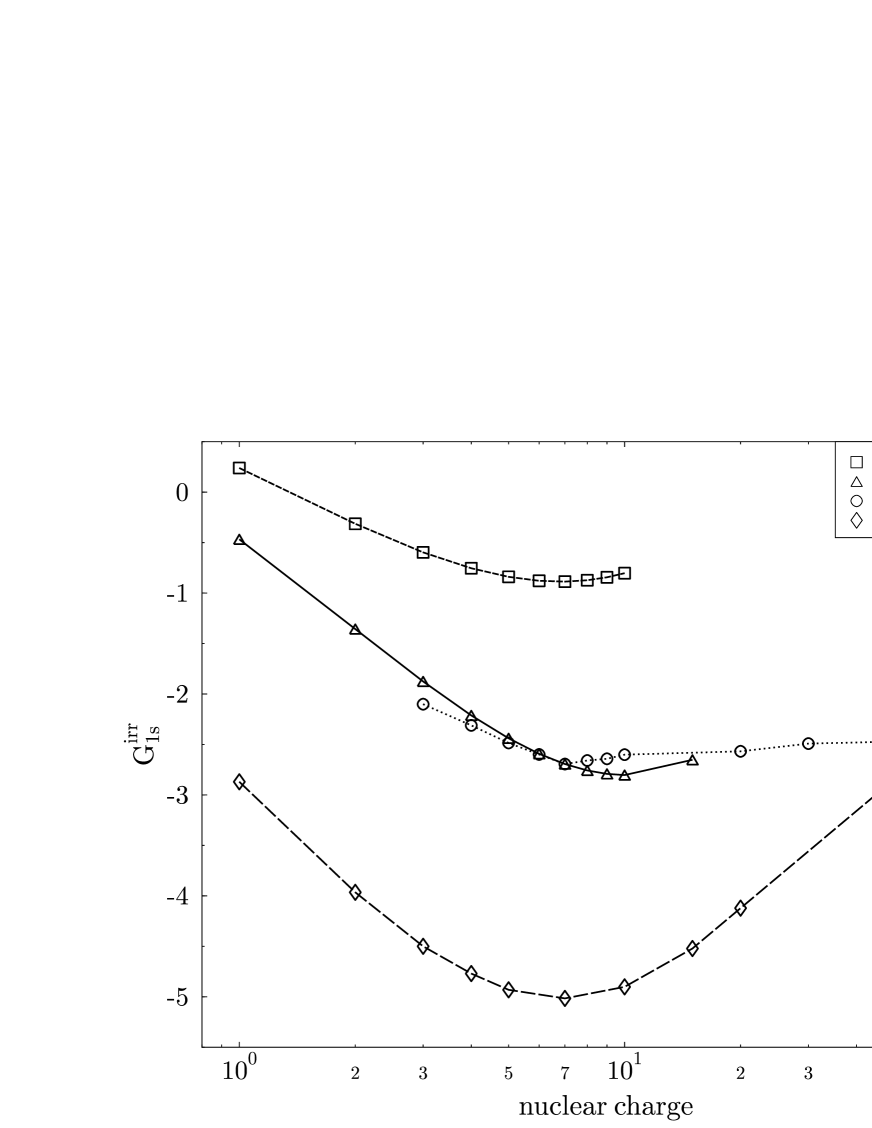
FIG. 2.: The function $G_{1s}^{\rm irr}(Z\alpha)$ in the different calculations.

TABLE I.: Convergence of the partial $\sum_{l}\Delta E^{(l)}_{1s}$ contributions in the first order self-energy $\Delta E_{1s}$ evaluation for $Z=10$. The number of the grid points was chosen to be $N=28$.

even				odd				$\Delta E_{1s}$ (eV)
$l$		$\sum_{l^{\prime}=0}^{l}\Delta E^{(l^{\prime})}_{1s}$ (eV)		$l$		$\sum_{l^{\prime}=1}^{l}\Delta E^{(l^{\prime})}_{1s}$ (eV)		This work		Ref. [16]
0		0.1269		1		0.1769		0.1688		0.1566
2		0.1615		3		0.1715
4		0.1659		5		0.1702
6		0.1672

TABLE II.: Comparison of the SESE (a) correction for the $1s$-ground state with previous calculations.

		$\Delta E^{\rm irr}_{1s}$ (eV)						$G^{\rm irr}_{1s}$
$Z$		Ref. [2]		Ref. [3]		This work		Ref. [3]		This work
3				$-0.6237\times 10^{-7}$		$-0.2913\times 10^{-7}$		$-4.50$		$-2.101$
4				$-0.2786\times 10^{-6}$		$-0.1351\times 10^{-6}$		$-4.77$		$-2.311$
5				$-0.8792\times 10^{-6}$		$-0.4431\times 10^{-6}$		$-4.931$		$-2.485$
6						$-0.1153\times 10^{-5}$				$-2.599$
7				$-0.4808\times 10^{-5}$		$-0.2584\times 10^{-5}$		$-5.016$		$-2.694$
8						$-0.4972\times 10^{-5}$				$-2.659$
9						$-0.8903\times 10^{-5}$				$-2.642$
10				$-0.2796\times 10^{-4}$		$-0.1483\times 10^{-4}$		$-4.9016$		$-2.601$
20				$-0.7525\times 10^{-3}$		$-0.4688\times 10^{-3}$		$-4.1217$		$-2.568$
30						$-0.3454\times 10^{-2}$				$-2.491$
50						$-0.4407\times 10^{-1}$				$-2.472$
70		$-0.2283$		$-0.2282$		$-0.2314$		$-2.3804$		$-2.413$
80		$-0.4474$		$-0.4472$		$-0.4512$		$-2.3923$		$-2.413$
92		$-0.9712$		$-0.9706$		$-0.9599$		$-2.581$		$-2.553$

REFERENCES

• [1] P. J. Mohr, G. Plunien, and G. Soff, Phys. Rep. 293, 227 (1998).
• [2] A. Mitrushenkov, L. Labzowsky, I. Lindgren, H. Persson, and S. Salomonson, Phys. Lett. A 200, 51 (1995).
• [3] S. Mallampalli and J. Sapirstein, Phys. Rev. Lett. 80, 5297 (1998).
• [4] S. Mallampalli and J. Sapirstein, Phys. Rev. A 57, 1548 (1998).
• [5] L. N. Labzowsky and A. O. Mitrushenkov, Phys. Lett. A 198, 333 (1995); Phys. Rev. A 53, 3029 (1996).
• [6] I. Lindgren, H. Persson, S. Salomonson, and P. Sunnergren, Phys. Rev. A 58, 1001 (1998).
• [7] H. Persson, I. Lindgren, and S. Salomonson, Phys. Scr. T 46, 125 (1993); I. Lindgren, H. Persson, S. Salomonson, and A. Ynnerman, Phys. Rev. A 47, R4555 (1993).
• [8] H. M. Quiney and I. P. Grant, Phys. Scr. T 46, 132 (1993); J. Phys. B 27, L299 (1994).
• [9] L. N. Labzowsky, I. A. Goidenko, and A. V. Nefiodov, J. Phys. B 31, L477 (1998).
• [10] Yu. Yu. Dmitriev, T. A. Fedorova, and D. M. Bogdanov, Phys. Lett. A 241, 84 (1998).
• [11] L. N. Labzowsky and I. A. Goidenko, J. Phys. B 30, 177 (1997); I. A. Goidenko and L. N. Labzowsky, Zh. Eksp. Teor. Fiz. 112, 1197 (1997) [Sov. Phys. JETP 85, 650 (1997)].
• [12] K. Pachucki, Phys. Rev. Lett. 72, 3154 (1994).
• [13] M. I. Eides and V. A. Shelyuto, Pis’ma Zh. Eksp. Teor. Fiz. 61, 465 (1995) [JETP Lett. 61, 478 (1995)]; Phys. Rev. A 52, 954 (1995).
• [14] S. G. Karshenboim, Zh. Eksp. Teor. Fiz. 103, 1105 (1993) [Sov. Phys. JETP 76, 541 (1993)].
• [15] W. R. Johnson, S. A. Blundell, and J. Sapirstein, Phys. Rev. A 37, 307 (1988).
• [16] P. J. Mohr, Phys. Rev. A 46, 4421 (1992).
• [17] S. Mallampalli and J. Sapirstein, (private communication).