Quantum–Classical Correspondence: Controlling Quantum Transport by State Synthesis in Ion Traps

Abstract

A procedure to enhance the quantum–classical correspondence even in situations far from the classical limit is proposed. It is based on controlling the quantum transport between classical regions using the capability to synthesize arbitrary motional states in ion traps. Quantum barriers and passages to transport can be created selecting the relevant frequencies. This technique is then applied to stabilize the quantum motion onto classical structures or alter the dynamical tunneling in nonintegrable systems.

Systems for which predictions can be made using classical mechanics can show quantum mechanical properties under suitable experimental conditions. The observables measured can be of a non-classical class as in Bell experiments. States can also be chosen to deviate from classical behavior, an idea that we will exploit in the present Letter. Despite this, the correspondence principle continues to be a guide to the study of the interrelation between quantum and classical mechanics, specially applied to the study of atomic and molecular systems [2]. More recently, a new class of experiments for which Hamiltonians can be engineered and detailed properties can be monitored have allowed to apply this correspondence in more detail. Cold atoms experiments have shown the possibility of inducing quantum dynamics with a particularly appealing classical limit, the $\delta$-kicked rotor. These experiments observed dynamical localization, accelerator modes and only recently the effect of noise and dissipation [3]. In addition there have been theoretical proposals of experimental configurations in ion traps to study dynamical localization [4], revivals [5] and state sensitivity [6, 7].

In this Letter we show how to enhance the quantum–classical correspondence by controlling and monitoring quantum transport in an ion trap. The control is achieved not only by engineering the Hamiltonian but most importantly by state synthesis. To monitor the relevant effects we use tomography and simpler alternative techniques. Trapped ions advantages to both control and monitor have already been used for the study of other aspects of quantum systems, like the quantum Zeno effect [8], possible nonlinear variants of quantum theory [9], reservoir engineering [10] and quantum computation [11].

To see the relative contribution of the classical backbone and the purely quantum effects consider the $Q$ distribution that it is measured in tomography [12]. Its continuity equation is of the form

$$\frac{\partial Q}{\partial t}+\{Q,H\}+Z(V,Q,t,\hbar)=0,$$ (1)

with $Q(\alpha;t)=|\langle\alpha|\Psi(t)\rangle|^{2}$, being $|\alpha\rangle$ a coherent state, $V$ the potential and $\{,\}$ the classical Poisson bracket. This continuity equation is the classical Liouville equation plus a quantum term $Z(V,Q,t,\hbar)$ given by $Z=-\frac{2}{\hbar}\rm{Im}\{\langle\Psi|\alpha\rangle V\left(x/2+i\hbar\partial/\partial p\right)\langle\alpha|\Psi\rangle\}$. An ideal experimental setup to study the quantum–classical correspondence would then have the possibility to control all three dependencies of $Z$, i.e., the potential, the quantum state and an effective Planck constant. Moreover, it should be possible to have measurable quantities showing the relative importance of classical and quantum contributions, e.g. the $Q$ distribution itself. All of the above conditions can be fulfilled in the case of an harmonically trapped ion. This is possible due to the interaction between the internal (electronic) and external (vibrational) degrees of freedom of the ion by means of laser pulses in resonant and non–resonant regimes [15].

In the quantum–classical boundary both the classical Liouville and the quantum terms in the continuity equation in (1) are relevant. The quantum contribution to the transport is state dependent and the final flow is diverted from the classical flow by an amount that depends on the quantum state. We first pick out the classical backbone structure and then study how to manipulate the quantum transport depending on the synthesized state. We need to construct a family of Hamiltonians that have regular, mixed or chaotic phase space. In the trapped ion setup we make use of the harmonic delta kicked Hamiltonian, first introduced in [6], describing a harmonic oscillator periodically perturbed by non–linear position dependent delta kicks. We consider a single trapped ion in a harmonic potential [15] with two internal levels $|e\rangle$ and $|g\rangle$ with transition frequency $\omega_{0}$ interacting with a time dependent laser pulse of near–resonant light of frequency $\omega_{L}$ which is rapidly and periodically switched. For sufficiently large detuning $\delta=\omega_{0}-\omega_{L}$ the excited state amplitude can be adiabatically eliminated. The Hamiltonian in this limit is given by [6]

$$H=H_{0}+K[\cos(2k_{L}x)+1]|g\rangle\langle g|\sum^{\infty}_{n=-\infty}\delta(t-n\tau),$$ (2)

where $H_{0}$ is the harmonic oscillator Hamiltonian, $K$ is the kick strength related to the laser beam power, $k_{L}=2\pi/\lambda$ the laser wave number, and $\tau$ the time between kicks. A particularly important parameter is the so–called Lamb–Dicke parameter $\eta=k_{L}\sqrt{\hbar/2m\nu}$, where $\nu$ is the oscillator frequency and $m$ the mass. Thus by varying $\eta$ it is possible to change the effective $\hbar$ of the system, i.e. doing it more classical.

In the following the relevance of the classical backbone is shown by predicting the time averaged quantum $Q$ function by means of classical theorems. We write the potential for a phase space region as $V=V_{0}+V_{1}$, with $V_{0}$ and $V_{1}$ the unperturbed an perturbed potentials that in general have different phase space topologies. The time averaged dynamics of an initially synthesized motional Fock state is shown to be predicted from knowledge of the classical solution for $V_{0}$ and the Kolmogorov-Arnold-Moser (KAM) and the Poincare-Birkoff (PB) theorems [16]. These two theorems in conjunction mean that, increasing the perturbation $V_{1}$, the phase space tori break in increasing irrationality values of the ratio of their winding numbers $r=\omega_{1}/\omega_{2}$ with $\omega_{1}$ and $\omega_{2}$ the two frequencies of a given torus [17]. When the winding number is sufficiently close to the rational number $l/s$ the torus breaks into alternative $ks$ stable and unstable points, with $k,l,s$ integers [16].

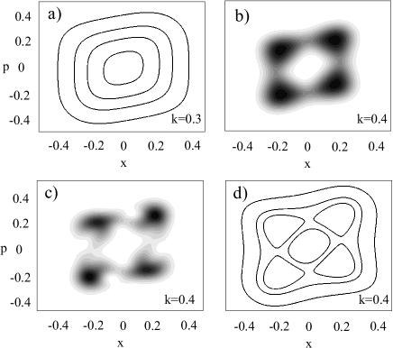
FIG. 1.: (a) Stroboscopic classical map with $k=0.3$. The rational number to which the winding number approaches is 1/4 for the initial condition (x,p)=(0.22,0). (b) $Q_{T}$ function with $k=0.4$ and $\eta=0.25$ (see text). (c) $Q$ function averaged over three different tomographic measurements after applying 21, 22 and 23 kicks. All parameters as before. (d) Stroboscopic classical map with $k=0.4$. $\nu\tau=1.8$ for all the cases. $x$ and $p$ are in units of $\lambda$ and $m\nu\lambda$ in all discussions and $k=\sqrt{2}K\eta^{2}/\hbar$.

Fig. 1(a) shows the classical stroboscopic map for $V_{0}$. Following the values of the winding number increasing the perturbation we determine which torus is breaking first. We thus predict the averaged quantum behavior with total potential $V=V_{0}+V_{1}$ using only the classical information from the values of the winding numbers with $V=V_{0}$ and the classical theorems. Then a $|n\rangle=|7\rangle$ Fock state is predicted to have an averaged $Q$ function with four maxima (minima) on the classically stable (unstable) points when increasing the perturbation of the system. Fig. 1(b) shows the time-averaged Q function

$$Q_{T}=\lim_{M\rightarrow\infty}\frac{1}{M\tau}\sum_{m=0}^{M-1}Q(m\tau)=\sum_{\mu}|\langle\alpha|\mu\rangle|^{2}|\langle\Psi|\mu\rangle|^{2},$$ (3)

with $|\mu\rangle$ the Floquet states fulfilling ${\hat{U}}(\tau)|\mu\rangle=e^{-i\epsilon_{\mu}}|\mu\rangle$, where ${\hat{U}}(\tau)$ is the time evolution operator referring to one period $\tau$ and $\Psi$ is a given initial state. The four predicted maxima are clear in this Figure. Fig. 1(c) displays the $Q$ function averaged at three consecutive times, as it could be measured experimentally using three tomographic measurements [12] showing the same structure [13]. The classical stroboscopic map for the perturbed case in Fig. 1(d) shows clearly that $Q_{T}$ reveals the classical backbone in many details. Any other Fock state prepared would scan in the same way different structures of this or alternative classical maps.

We now propose to go a step further in the study of the quantum–classical correspondence controlling the relevance of the quantum and classical terms in (1) by state synthesis. We want to prepare a state initially localized in a classical region $A$ with a barrier or a passage for transport to a different classical region $B$. Take as a starting state a coherent state localized on $A$, $\phi_{A}(0)$. Its averaged transport to region $B$, represented by another state $\phi_{B}$, is given by $P(|\phi_{A}\rangle,|\phi_{B}\rangle)=\lim_{M\rightarrow\infty}\frac{1}{M\tau}\sum_{m=0}^{M-1}|\langle\phi_{B}|\phi_{A}(m\tau)\rangle|^{2}$, that we can write as $P(|\phi_{A}\rangle,|\phi_{B}\rangle)=\sum_{\mu}|\langle\phi_{B}|\mu\rangle|^{2}|\langle\phi_{A}(0)|\mu\rangle|^{2}$ using the Floquet basis. For $P(|\phi_{A}\rangle,|\phi_{B}\rangle)$ not to be zero, the states $\phi_{A}(0)$ and $\phi_{B}$ must have nonzero overlap with common Floquet states denoted as $\{|\mu\rangle_{A\cap B}\}$. To form a new state that minimizes, $\varphi_{A^{\prime}}^{-B}$, or maximizes, $\varphi_{A^{\prime}}^{+B}$, the transport to region $B$ we eliminate (enhance) from $\phi_{A}(0)$ the Floquet components $\{\mu_{A\cap B}\}$ as

$$|\varphi_{A^{\prime}}^{\pm B}\rangle=N_{1}(|\phi_{A}(0)\rangle\pm\sum_{\mu_{A\cap B}}r_{\mu}|\mu\rangle\langle\mu|\phi_{A}(0)\rangle),$$ (4)

with $r_{\mu}=0$ or $1$ when the corresponding weight $|\langle\mu|\phi_{A}\rangle|^{2}$ is smaller or greater than a value $c_{\rm tol}$, respectively and $N_{i}$ will be normalization constants from now on. The value $c_{\rm tol}$ is chosen to be the minimum possible subject to the condition that the new region $A^{\prime}$ is sufficiently close to the initial region of localization $A$. We propose then the synthesis of the states

$$|\Psi_{A^{\prime}}^{\pm B}\rangle=N_{2}\sum_{n=0}^{n_{\rm exp}}|n\rangle\langle n|\varphi_{A^{\prime}}^{\pm B}\rangle,$$ (5)

with $\{|n\rangle\}$ the Fock basis and where we consider only an experimentally feasible maximum number of Fock states $n_{\rm exp}$ [18] and amplitudes $\langle n|\varphi_{A^{\prime}}^{\pm B}\rangle$ chosen to approximate the theoretical state (4).

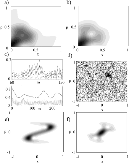
FIG. 2.: (a) $Q_{T}$ function for $\phi_{A}$ coherent state. (b) $Q_{T}$ function for modified $\Psi_{A^{\prime}}^{-B}$ state. (c) Upper Plot. Correlation function for $\phi_{A}$, $\Psi_{A^{\prime}}^{-B}$ (dot) and $\Psi_{A^{\prime}}^{+B}$ (dashed). Lower Plot. Autocorrelation function for $\Psi_{A^{\prime}}^{\rm sta}$ state and $\phi_{A}$ coherent state (dot). (d) Stroboscopic classical map. (e) $Q$ for a initial coherent state centered at $(x_{A},p_{A})=(0,0)$ after two kicks. (f) As before for a $\Psi_{A^{\prime}}^{\rm sta}$ state. All figures obtained with the parameters: $k=2.7$, $\nu\tau=1.7$ and $\eta=.5$. See text for more details of each case.

The enhanced quantum–classical correspondence is thus obtained even far from the classical limit by choosing classical regions $A$ and $B$ and controlling the transport between them as described above. Some comments for this construction are necessary: (a) We can give up the condition that the initial state must be localized in region $A^{\prime}$ slightly bigger than the region $A$ of the minimum uncertainty wavepacket. For some experiments it is interesting to have a larger variance of the initial state or an additional localization in a different region $A^{\prime\prime}$. (b) If we only want to modify the transport to region $B$ and not to other regions $C$ we have to use $r_{\mu}=0$ in (4) for the Floquet states that have important overlap with a state $\phi_{C}$ centered on $C$. (c) The states localized in the regions $A$, $B$ and $C$ do not need in general to be minimum uncertainty states but we have the freedom to use any states related to these phase space regions.

We now discuss first a general example of modified transport properties of a given state and we then study stabilization, and modification of dynamical tunneling as two interesting examples. We want to synthesize a state $\Psi_{A^{\prime}}^{-B}$ initially localized on $(x_{A},p_{A})=(0.1,0.2)$ that avoids transport to $(x_{B},p_{B})=(0.3,0.3)$. We use coherent states for $\phi_{A}$ and $\phi_{B}$ and a value $c_{\rm tol}=0.001$ so all the Floquet states with important overlap with $\phi_{B}$ have $r_{\mu}=1$ in (4). An experimentally realizable state with $n_{\rm exp}=10$ can be constructed with overlap $|\langle\Psi_{A^{\prime}}^{-B}|\varphi_{A^{\prime}}^{-B}\rangle|^{2}=0.9$ to the theoretical state. Despite both wavefunctions $\langle\alpha|\phi_{A}\rangle$ and $\langle\alpha|\Psi_{A^{\prime}}^{-B}\rangle$ being initially localized around $A$, with $|\langle\phi_{A}|\Psi_{A^{\prime}}^{-B}\rangle|^{2}=0.82$, it is clear from Fig. 2(a) and (b) that their $Q_{T}$ functions are very different. The $Q_{T}$ function for $\Psi_{A^{\prime}}^{-B}$ shows a clear hole at the location $B$, in contrast to the minimum uncertainty state $\phi_{A}$. The correlation function $P(m\tau)=|\langle\phi_{B}|\hat{U}^{m}(\tau)|\Phi\rangle|^{2}$ is shown in Fig. 2(c) for $\Phi=\phi_{A}$ and $\Psi_{A^{\prime}}^{-B}$, the latter showing a significant decrease. These correlation functions can be measured experimentally by applying a displacement associated to $\phi_{B}$ and then measuring the Fock ground state population both steps possible to implement in a trap [14]. Successful results can also be obtained for the state $\Psi_{A^{\prime}}^{+B}$ that presents a maximum on region $B$ in $Q_{T}$, see Fig. 2(c).

Particular instances of the states $\Psi_{A^{\prime}}^{\pm B}$ are of special relevance. The stabilization of the vibration of the ion can be understood as a modified transport problem. In this case $A$ is the region of localization and $B$ the rest of the phase space and we are interested in constructing a state $\Psi_{A^{\prime}}^{-B}$ that we will name for the stabilization case as $\Psi_{A^{\prime}}^{\rm sta}$. An alternative way to understand expression (5) for this situation now in terms of the dynamics is given in the following. The autocorrelation function of a typical state $|\langle\phi_{A}(0)|\phi_{A}(t)\rangle|^{2}$ will show an initial maximum (however small) at $t_{M}>0$. We can now clean the state $\phi_{A}$ of the Floquet components that do not contribute to this maximum and therefore create a new state stabilized on $A$. Note first that a particular Floquet state $|\mu_{0}\rangle$ can be obtained from the time-dependent vector $|\phi_{A}(t)\rangle=\sum_{\mu}|\mu\rangle\langle\mu|\phi_{A}(0)\rangle\exp(-i\epsilon_{\mu}t)$ (a solution of the Schrödinger equation only for $t=m\tau$) as $|\mu_{0}\rangle\propto\lim_{T\rightarrow\infty}G_{T,\mu_{0}}$ with $G_{T,\mu_{0}}\equiv\int_{-T}^{T}dt\ |\phi_{A}(t)\rangle\exp(i\epsilon_{\mu_{0}}t)$. A state related to the short term dynamics is then $G_{t_{M},\omega_{0}}$ with $\omega_{0}$ the value of $\omega$ that makes $S(\omega)=\int_{-t_{M}}^{t_{M}}dt\langle\phi_{A}(0)|\phi_{A}(t)\rangle\exp(i\omega t)$ a maximum [19]. This state $G_{t_{M},\omega_{0}}$ can then be approximated as

$$|\varphi_{A^{\prime}}^{\rm sta}\rangle=N_{3}\sum_{\mu_{\rm sta}}|\mu\rangle\langle\mu|\phi_{A}(0)\rangle,$$ (6)

with $\mu_{\rm sta}$ the Floquet eigenfrequencies in the interval $\omega_{0}-\frac{\pi}{t_{M}}<\omega<\omega_{0}+\frac{\pi}{t_{M}}$ with a weight $|\langle\mu|\phi_{A}(0)\rangle|^{2}>a_{\rm sta}$. The value of $a_{\rm sta}$ is chosen maximum with the requirement than the state $\varphi_{A^{\prime}}^{\rm sta}$ has a tolerable localization around $A$. The state $\Psi_{A^{\prime}}^{\rm sta}$ in (5) synthesized to approximate $\varphi_{A^{\prime}}^{\rm sta}$ will then show an initial localization around $A$ because it selects the short term dynamics and will recur continuously to $A$ because it is made of very few selected Floquet states. In fact there are several maxima in $S(\omega)$ and we can choose the value $\omega_{0}$ with minimum number of Floquet states maximizing stabilization in this way.

Using this stabilization procedure we have found enhanced localization onto KAM tori, islands of size smaller than the effective $\hbar$, cantori or unstable periodic orbits effects [20]. The following example of enhanced localization onto a classical unstable orbit can be realized experimentally. We consider the stroboscopic map in Fig. 2(d). Fig. 2(e) shows the $Q$ function for a initial minimum uncertainty state, $\phi_{A}$, after two kicks centered at $(x_{A},p_{A})=(0,0)$. The state is spread from an unstable periodic orbit along the unstable manifold. The stabilization is achieved in this case with a state $\Psi_{A^{\prime}}^{\rm sta}$ centered on the middle of the chaotic region at $(0,0)$ with $|\langle\varphi^{\rm sta}_{A^{\prime}}|\Psi^{\rm sta}_{A^{\prime}}\rangle|^{2}=0.72$ and $n_{\rm exp}=12$, a single Floquet state. The stabilization achieved is clearly seen in the measurable autocorrelation function [14], see Fig. 2(c) and Fig. 2(f) for the $Q$ function of such stabilized state. This example constitutes a realizable experiment to directly observe a quantum scar. [21]

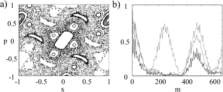
FIG. 3.: (a) Stroboscopic classical map with $k=1.2$ and $\nu\tau=2\pi/3$. (b) Autocorrelation function for an initial coherent state, Floquet doublet (dot), and $|\Psi^{B}_{A^{\prime}}\rangle$ state (dash). Parameters as before with $\eta=0.5$.

As a final example we show how to increase the dynamical tunneling associated to classically forbidden regions, see Fig. 3(a). An initial minimum uncertainty state located at $(x_{A},p_{A})=(-0.6,0)$ has dynamical tunneling and contributions from a unstable periodic orbit located at $(x_{B},p_{B})=(-0.5,0.3)$. A state (4) eliminating the contributions of $B$ is mainly composed of three Floquet doublets reflecting the oscillations due to quantum tunneling. The autocorrelation function is shown in Fig. 3(b) for a state (5) with $|\langle\varphi^{B}_{A^{\prime}}|\Psi^{B}_{A^{\prime}}\rangle|^{2}=0.85$. This can be measured by applying displacements associated to the initial regions of localization or more directly by inverting the unitary process which created the initial state. An example of stabilization in this case is choosing a state made of a single doublet where $|\langle\varphi^{\rm sta}_{A^{\prime}}|\Psi^{\rm sta}_{A^{\prime}}\rangle|^{2}=0.8$. In this case the oscillations due to the tunneling are more clearly reflected. Both states with $n_{\rm exp}=25$ since their location in phase space implies higher Fock state contributions than previous cases. Choosing different doublets would give rise to different tunneling times. Finally notice that by increasing $n_{\rm exp}$, i.e. the overlap to the theoretical state, all features discussed in previous examples will be more dramatically shown [18].

In conclusion, we have presented a way to enhance the quantum–classical correspondence by modifying quantum transport in an ion trap. We have specially made use of the ability to synthesize arbitrary states of motion in a ion trap.

G.G.P. acknowledges a Marie Curie Fellowship. J.F.P. is supported by the European TMR network ERB-4061-PL-95-1412 and specially dedicates this paper to M.B.

REFERENCES

- [1] Both authors contributed equally.
- [2] A. Peres, Quantum Theory: Concepts and Methods (Kluwer Academic Publishers, Dordrecht, 1993).
- [3] F. L. Moore et al., Phys. Rev. Lett. 73, 2974 (1994); F. L. Moore et al., ibid 75, 4598 (1997); H. Ammann et al., ibid 80, 4111 (1998); B. G. Klappauf et al., ibid 81, 1203 (1998).
- [4] M. El Ghafar et al., Phys. Rev. Lett. 78, 4181 (1997); G.P. Berman et al, quant-ph/9903063.
- [5] J. K. Breslin et al., Phys. Rev. A 56, 3022 (1997).
- [6] S. A. Gardiner et al., Phys. Rev. Lett. 79, 4790 (1997).
- [7] G. García de Polavieja, Phys. Rev. A 57, 3184 (1998).
- [8] W. M. Itano et al., Phys. Rev. A 41, 2295 (1990).
- [9] J. J. Bollinger et al., Phys. Rev. Lett. 63, 1031 (1989).
- [10] J. F. Poyatos et al., Phys. Rev. Lett. 77, 4728 (1996).
- [11] J. I. Cirac and P. Zoller, Phys. Rev. Lett. 74, 4094 (1995) C. Monroe et al., Phys. Rev. Lett. 75, 4714 (1995).
- [12] D. Leibfried et al., Phys. Rev. Lett. 77, 4281 (1996).
- [13] Simulations have been calculated in a truncated Fock basis. Convergence was verified by variation of the cutoff.
- [14] J. F. Poyatos et al., Phys. Rev. A. 54, R1966 (1996);
- [15] D. J. Wineland et al., J. Res. Natl. Inst. Stand. Technol. 103, 259 (1998); Forschr. Phys. 46, 363, (1998).
- [16] M. Tabor, Chaos and integrability in nonlinear dynamics (John Wiley and sons, 1989).
- [17] The dynamics associated to the harmonic delta kick is best described in terms of a two–dimensional Poincaré surface of section where only two frequencies are involved.
- [18] Experimentally Fock states has been synthesized up to (). See D. M. Meekhof et al., Phys. Rev. Lett. 76, 1796 (1996). However, recent theoretical proposals to prepare arbitrary quantum states work with significantly higher Fock states, e.g. , and higher Lamb–Dicke parameters. These proposals seem to be possible with actual or near future technology. See S. A. Gardiner et al., Phys. Rev. A. 55, 1683 (1997); B. Kneer and C. K. Law, ibid, 57, 2096 (1998).
- [19] G. García de Polavieja et al., Phys. Rev. Lett. 73, 1613 (1994).
- [20] J. F. Poyatos and G. García de Polavieja, unpublished.
- [21] E. J. Heller, Phys. Rev. Lett. 53, 1515 (1984).