Sonoluminescence as a QED vacuum effect.
I: The Physical Scenario

Abstract

Several years ago Schwinger proposed a physical mechanism for sonoluminescence in terms of changes in the properties of the quantum-electrodynamic (QED) vacuum state during collapse of the bubble. This mechanism is most often phrased in terms of changes in the Casimir Energy (i.e., changes in the distribution of zero-point energies) and has recently been the subject of considerable controversy. The present paper further develops this quantum-vacuum approach to sonoluminescence: We calculate Bogolubov coefficients relating the QED vacuum states in the presence of a homogeneous medium of changing dielectric constant. In this way we derive an estimate for the spectrum, number of photons, and total energy emitted. We emphasize the importance of rapid spatio-temporal changes in refractive indices, and the delicate sensitivity of the emitted radiation to the precise dependence of the refractive index as a function of wavenumber, pressure, temperature, and noble gas admixture. Although the basic physics of the dynamical Casimir effect is a universal  phenomenon of QED, specific and particular experimental features are encoded in the condensed matter physics controlling the details of the refractive index. This calculation places rather tight constraints on the possibility of using the dynamical Casimir effect as an explanation for sonoluminescence, and we are hopeful that this scenario will soon be amenable to direct experimental probes. In a companion paper we discuss the technical complications due to finite-size effects, but for reasons of clarity in this paper we confine attention to bulk effects.

I Introduction

Sonoluminescence (SL) is the phenomenon of light emission by a sound-driven gas bubble in fluid [5]. In SL experiments the intensity of a standing sound wave is increased until the pulsations of a bubble of gas trapped at a velocity node have sufficient amplitude to emit brief flashes of light having a “quasi-thermal” spectrum with a “temperature” of several tens of thousands of Kelvin. The basic mechanism of light production in this phenomenon is still highly controversial. We first present a brief summary of the main experimental data (as currently understood) and their sensitivities to external and internal conditions. For a more detailed discussion see [5].

SL experiments usually deal with bubbles of air in water, with ambient radius $R_{\mathrm{a}mbient}\approx 4.5\;\mu{\rm m}$. The bubble is driven by a sound wave of frequency of 20–30 kHz. (Audible frequencies can also be used, at the cost of inducing deafness in the experimental staff.) During the expansion phase, the bubble radius reaches a maximum of order $R_{\mathrm{m}ax}\approx\;45\;\mu{\rm m}$, followed by a rapid collapse down to a minimum radius of order $R_{\mathrm{m}in}\approx 0.5\;\mu{\rm m}$. The photons emitted by such a pulsating bubble have typical wavelengths of the order of visible light. The minimum observed wavelengths range between $200\;{\rm nm}$ and $100\;{\rm nm}$. This light appears distributed with a broad-band spectrum. (No resonance lines, roughly a power-law spectrum with exponent depending on the noble gas admixture entrained in the bubble, and with a cutoff in the extreme ultraviolet.) For a typical example, see figures 1 and 2. If one fits the data to a Planck black-body spectrum the corresponding temperature is several tens of thousands of Kelvin (typically $70,000\;{\rm K}$, though estimates varying from $40,000\;{\rm K}$ to $100,000\;{\rm K}$ are common). There is considerable doubt as to whether or not this temperature parameter corresponds to any real physical temperature. There are about one million photons emitted per flash, and the time-averaged total power emitted is between $30$ and $100\;\hbox{ mW}$.

The photons appear to be emitted by a very tiny spatio-temporal region: Estimated flash widths vary from less than $35\;{\rm ps}$ to more than $380\;{\rm ps}$ depending on the gas entrained in the bubble [6, 7]. There are model-dependent (and controversial) claims that the emission times and flash widths do not depend on wavelength [7]. As for the spatial scale, there are various model-dependent estimates but no direct measurement is available [7]. Though it is clear that there is a frequency cutoff at about $1\;{\rm PHz}$ the physics behind this cutoff is controversial. Standard explanations are (1) a Thermal cutoff (deprecated because the observed cutoff is much sharper than exponential) , or (2) the opacity of water in the UV (deprecated because of the observed absence of dissociation effects). Alternatively, Schwinger suggests that the critical issue is that (3) the real part of the refractive index of water goes to unity in the UV (so that there is no change in the Casimir energy during bubble collapse). We shall add another possible contribution to the mix: (4) a rapidly changing refractive index causes photon production with an “adiabatic cutoff’ that depends on the timescale over which the refractive index changes. (Because the observed falloff above the physical cutoff is super-exponential it is clear that this adiabatic effect is at most part of the complete picture.)

FIG. 1.: Typical experimental spectrum: The data has been extracted from figure 51 of reference 1, and has here been plotted as intensity (arbitrary units) as a function of wavelength. Note that no data has been taken at frequencies below the visible range. The spectrum is a broad-band spectrum without significant structure. The physical nature of the cutoff (which occurs in the far ultraviolet) is one of the key issues under debate.

FIG. 2.: Typical experimental spectrum: The data has been extracted from figure 51 of reference 1, and has here been plotted as a number spectrum as a function of frequency.

Any truly successful theory of SL must also explain a whole series of characteristic sensitivities to different external and internal conditions. Among these dependencies the main one is surely the mysterious catalytic role of noble gas admixtures. (Most often a few percent in the air entrained in the bubble. One can obtain SL from air bubbles with a $1\%$ content of argon, and also from pure noble gas bubbles, but the phenomenon is practically absent in pure oxygen bubbles.) In fact, it has been suggested that physical processes concentrate the noble gasses inside the bubble to the extent that the bubble consists of almost pure noble gas [8], and some experimental results seem to corroborate this suggestion [9].

Other external conditions that influence SL are: (1) Magnetic Fields — If the frequency of the driving sound wave is kept fixed, SL disappears above a pressure-dependent threshold magnetic field: $H\geq H_{0}(p)$. On the other hand, for a fixed value of the magnetic field $H_{0}$, there are both upper and lower bounds on the applied pressure that bracket the region of SL, and these bounds are increasing functions of the applied magnetic field [10]. This is often interpreted as suggesting that the primary effect of magnetic fields is to alter the condition for stable bubble oscillations. See. also [11]. (2) Temperature of the water — If $T_{H_{2}O}$ decreases then the emitted power $W$ increases. The position of the peak of the spectrum depends on $T_{H_{2}O}$. It has been suggested that the increased light emission at lower water temperature is associated with an increased stability of the bubble, allowing for higher driving pressures [12].

These are only the most salient features of the SL phenomenon. In attempting to explain such detailed and specific behaviour the dynamical Casimir approach (QED vacuum approach) encounters the same problems as all other approaches have. Nevertheless we shall argue that SL explanations using a Casimir-like framework are viable, and merit further investigation.

In this paper we shall concentrate on changes in the QED vacuum state as a candidate explanation for SL, and try to clear up considerable confusion as to what models based on the Casimir effect do and do not predict. It is important to realize that changes in the static Casimir energy in this experimental situation are big, that they have roughly the right energy budget to drive SL, and that any purported non-Casimir explanation for SL will have to find a way to hide the effects of these changes in Casimir energy so as to make them unobservable.

II Quantum-electrodynamic models of SL

A Quasi-static Casimir models: Schwinger’s approach

The idea of a “Casimir route” to SL is due to Schwinger who several years ago wrote a series of papers [13, 14, 15, 16, 17, 18, 19] regarding the so-called dynamical Casimir effect. Considerable confusion has been caused by Schwinger’s choice of the phrase “dynamical Casimir effect” to describe his particular model. In fact, Schwinger’s original model is not dynamical but is instead quasi-static as the heart of the model lies in comparing two static Casimir energy calculations: That for an expanded bubble with that for a collapsed bubble. One key issue in Schwinger’s model is thus simply that of calculating Casimir energies for dielectric spheres—and there is already considerable disagreement on this issue. A second and in some ways more critical question is the extent to which this difference in Casimir energies may be converted to real photons during the collapse of the bubble—it is this issue that we shall address in this paper. The original quasi-static incarnation of the Schwinger model had no real way of estimating either photon production efficiency or timing information (when does the flash occur?). In contrast the model of Eberlein [20, 21, 22] (more fully discussed below) is truly dynamical but uses a much more specific physical approximation—the adiabatic approximation. The two models should not be confused. In this paper we shall argue that the observed features of SL force one to make the sudden approximation. We can then estimate the spectrum of the emitted photons by calculating an appropriate Bogolubov coefficient relating two states of the QED vacuum. The resulting variant of the Schwinger model for SL is then rather tightly constrained, and should be amenable to experimental verification (or falsification) in the near future.

In his series of papers [13, 14, 15, 16, 17, 18, 19] on SL, Schwinger showed that the dominant bulk contribution to the Casimir energy of a bubble (of dielectric constant $\epsilon_{\mathrm{i}nside}$) in a dielectric background (of dielectric constant $\epsilon_{\mathrm{o}utside}$) is [16]

$$E_{\mathrm{c}avity} = +2\frac{4\pi}{3}R^{3}\;\int_{0}^{K}{4\pi k^{2}dk\over(2\pi)^{3}}\;\frac{1}{2}\hbar ck\left({1\over\sqrt{\epsilon_{\mathrm{i}nside}}}-{1\over\sqrt{\epsilon_{\mathrm{o}utside}}}\right)+\cdots$$ (1)

$$= +\frac{1}{6\pi}\hbar cR^{3}K^{4}\left({1\over\sqrt{\epsilon_{\mathrm{i}nside}}}-{1\over\sqrt{\epsilon_{\mathrm{o}utside}}}\right)+\cdots.$$ (2)

The corresponding number of emitted photons is

$$N = +2\frac{4\pi}{3}R^{3}\;\int_{0}^{K}{4\pi k^{2}dk\over(2\pi)^{3}}\;\frac{1}{2}\left(\frac{\sqrt{\epsilon_{\mathrm{o}utside}}}{\sqrt{\epsilon_{\mathrm{i}nside}}}-1\right)+\cdots$$ (3)

$$= +\frac{2}{9\pi}(RK)^{3}\left(\frac{\sqrt{\epsilon_{\mathrm{o}utside}}}{\sqrt{\epsilon_{\mathrm{i}nside}}}-1\right)+\cdots.$$ (4)

Here we have inserted an explicit factor of two with respect to Schwinger’s papers to take into account both photon polarizations. There are additional sub-dominant finite volume effects discussed in [23, 24, 25]. Schwinger’s result can also be rephrased in the clearer and more general form as [23, 24, 25]:

$$E_{\mathrm{c}avity}=+2V\int\frac{d^{3}\vec{k}}{(2\pi)^{3}}\;\frac{1}{2}\hbar\left[\omega_{\mathrm{i}nside}(k)-\omega_{\mathrm{o}utside}(k)\right]+\cdots$$ (5)

$$N=+2V\int\frac{d^{3}\vec{k}}{(2\pi)^{3}}\;\frac{1}{2}\left[{\omega_{\mathrm{i}nside}(k)\over\omega_{\mathrm{o}utside}(k)}-1\right]+\cdots$$ (6)

Here it is evident that the Casimir energy can be interpreted as a difference in zero point energies due to the different dispersion relations inside and outside the bubble. The quantity $K$ appearing above is a high-wavenumber cutoff that characterizes the wavenumber at which the (real part of) the refractive indices ($n=\sqrt{\epsilon}$) drop to their vacuum values. It is important to stress that this cutoff it is not a regularization artifact to be removed at the end of the calculation. The cutoff has a true physical meaning in its own right.

The three main points of strength of models based on zero point fluctuations (e.g., Schwinger’s model and its variants) are:

1) One does not need to achieve “real” temperatures of thousands of Kelvin inside the bubble. As discussed in [26], quasi-thermal behaviour is generated in quantum vacuum models by the squeezed nature of the two photon states created [21], and the “temperature” parameter is a measure of the squeezing, not a measure of any real physical temperature. (Of course, one should remember that the experimental data merely indicates an approximately power-law spectrum [$N(\omega)\propto\omega^{\alpha}$] with some sort of cutoff in the ultraviolet, and with an exponent that depends on the gases entrained in the bubble; the much-quoted “temperature” of the SL radiation is merely an indication of the scale of this cutoff $K$.)

2) There is no actual production of far ultraviolet photons (because the refractive index goes to unity in the far ultraviolet) so one does not expect dissociation effects in water that other models imply. Models based on the quantum vacuum automatically provide a cutoff in the far ultraviolet from the behaviour of the refractive index—this observation going back to Schwinger’s first papers on the subject.

3) One naturally gets the right energy budget. For $n_{\mathrm{o}utside}\approx 1.3$, $n_{\mathrm{i}nside}\approx 1$, $K$ in the ultra-violet, and $R\approx R_{\mathrm{m}ax}$, the change in the static Casimir energy approximately equals the energy emitted each cycle.

This last point is still the object of heated debate. Milton [27], and Milton and Ng [28, 29] strongly criticize Schwinger’s result claiming that actually the Casimir energy contains at best a surface term, the bulk term being discarded via (what is to our minds) a physically dubious renormalization argument. In their more recent paper [29] they discard even the surface term and now claim that the Casimir energy for a dielectric bubble is of order $E\approx\hbar c/R$. (The dispute is ongoing—see [30].) These points have been discussed extensively in [23, 24, 25] where it is emphasized that one has to compare two different physical configurations of the same system, corresponding to two different geometrical configurations of matter, and thus must compare two different quantum states defined on the same spacetime. In a situation like Schwinger’s model for SL one has to subtract from the zero point energy (ZPE) for a vacuum bubble in water the ZPE for water filling all space. It is clear that in this case the bulk term is physical and must be taken into account. Surface terms are also present, and eventually other higher order correction terms, but they prove to not be dominant for sufficiently large cavities [25].

The calculations of Brevik et al [32] and Nesterenko and Pirozhenko [33] also fail to retain the known bulk volume term. In this case the subtlety in the calculation arises from neglecting the continuum part of the spectrum. They consider a dielectric sphere in an infinite dielectric background and sum only over the discrete part of the spectrum to calculate their Casimir “energy”. When the continuum modes are reintroduced the proper volume dependence is recovered. Their conclusions regarding the relevance of the Casimir effect to SL are then incorrect: by completely discarding the volume (and indeed surface) contribution they are left with a Casimir “energy” that can be simply estimated by dimensional analysis to be of order $\hbar c/R$ and is strictly proportional to the inverse radius of the bubble. This is certainly a very small quantity insufficient to drive SL but this is also not the correct physical quantity to calculate. For a careful discussion of the correct identification of the physically relevant Casimir energy see [23, 24, 25].

While we believe that the contentious issues of how to define the Casimir energy are successfully dealt with in [23, 24, 25], one of the subsidiary aims of this paper is to side-step this whole argument and provide an independent calculation demonstrating efficient photon production.

In contrast to the points of strength outlined above, the main weakness of the original quasi-static version of Schwinger’s idea is that there is no real way to calculate either timing information or conversion efficiency. A naive estimate is to simply and directly link power produced to the change in volume of the bubble. As pointed out by Barber et al. [5], this assumption would imply that the main production of photons may be expected when the the rate of change of the volume is maximum, which is experimentally found to occur near the maximum radius. In contrast the emission of light is experimentally found to occur near the point of minimum radius, where the rate of change of area is maximum. All else being equal, this would seem to indicate a surface dependence and might be interpreted as a true weakness of the dynamical Casimir explanation of SL. In fact we shall show that the situation is considerably more complex than might naively be thought. We claim that there is much more going on than a simple change in volume of the bubble, and shall shortly focus attention on the “bounce” that occurs as the contents of the bubble hit the van der Waals hard core maximum density.

B Eberlein’s dynamical model for SL

The quantum vacuum approach to SL was developed extensively in the work of Eberlein [20, 21, 22]. The basic mechanism in Eberlein’s approach is a particular implementation of the dynamical Casimir effect: Photons are assumed to be produced due to an adiabatic change of the refractive index in the region of space between the minimum and the maximum bubble radius (a related discussion for time-varying but spatially-constant refractive index can be found in the discussion by Yablonovitch[34]). This physical framework is actually implemented via a boundary between two dielectric media which accelerates with respect to the rest frame of the quantum vacuum state. The change in the zero-point modes of the fields produces a non-zero radiation flux. Eberlein’s contribution was to take the general phenomenon of photon generation by moving dielectric boundaries and attempt a specific implementation of these ideas as a candidate for explaining SL.

It is important to realize that this is a second-order effect. Though he was unable to provide a calculation to demonstrate it, Schwinger’s original discussion is posited on the direct conversion of zero point fluctuations in the expanded bubble vacuum state into real photons plus zero point fluctuations in the collapsed bubble vacuum state. Eberlein’s mechanism is a more subtle (and much weaker) effect involving the response of the atoms in the dielectric medium to acceleration through the zero-point fluctuations. The two mechanisms are quite distinct and considerable confusion has been engendered by conflating the two mechanisms. Criticisms of the Eberlein mechanism do not necessarily apply to the Schwinger mechanism, and vice versa.

In the Eberlein analysis the motion of the bubble boundary is taken into account by introducing a velocity-dependent perturbation to the usual EM Hamiltonian:

$$H_{\epsilon} \!= \!\frac{1}{2}\int{\rm d}^{3}{\bf r}\left({{\bf D}^{2}\over\epsilon}+{\bf B}^{2}\right)\;,$$ (7)

$$\Delta H \!= \!\beta\int{\rm d}^{3}{\bf r}\frac{\epsilon-1}{\epsilon}\;({\bf D}\wedge{\bf B})\cdot{\bf\hat{r}}\;.$$ (8)

This is an approximate low-velocity result coming from a power series expansion in the speed of the bubble wall $\beta=\dot{R}/c$. The bubble wall is known to collapse with supersonic velocity, values of Mach 4 are often quoted, but this is still completely non-relativistic with $\beta\approx 10^{-5}$. Unfortunately, when the Eberlein formalism is used to model the observed quantity of radiation from each SL flash the implied bubble wall velocities are superluminal, indicating that one has moved outside the region of validity of the approximation scheme [35].

The Eberlein approach consists of a novel mixture of the standard adiabatic approximation with perturbation theory. In principle, the adiabatic approximation requires the knowledge of the complete set of eigenfunctions of the Hamiltonian for any allowed value of the parameter. In the present case only the eigenfunctions of part of the Hamiltonian, namely those of $H_{\epsilon}$, are known. (And these eigenfunctions are known explicitly only in the adiabatic approximation where $\epsilon$ is treated as time-independent.) The calculation consists of initially invoking the standard application of the adiabatic approximation to the full Hamiltonian, then formally calculating the transition coefficients for the vacuum to two photon transition to first order in $\beta$, and finally in explicitly calculating the radiated energy and spectral density. In this last step Eberlein used an approximation valid only in the limit $kR\gg 1$ which means in the limit of photon wavelengths smaller than the bubble radius. (Compare this with our discussion of the large $R$ limit below.) This implies that the calculation will completely miss any resonances that are present.

Eberlein’s final result for the energy radiated over one acoustic cycle is:

$${\cal W}=1.16\>\frac{(n^{2}-1)^{2}}{n^{2}}\,\frac{1}{480\pi}\left[{\hbar\over c^{3}}\right]\int_{0}^{T}{\rm d}\tau\;\frac{\partial^{5}R^{2}(\tau)}{\partial\tau^{5}}\,R(\tau)\beta(\tau)\;.$$ (9)

Eberlein approximates $n_{\mathrm{i}nside}\approx n_{\mathrm{a}ir}\approx 1$ and sets $n_{\mathrm{o}utside}=n_{\mathrm{w}ater}\to n$. The $1.16$ is the result of an integration that has to be estimated numerically. The precise nature of the semi-analytic approximations made as prelude to performing the numerical integration are far from clear.

One of the interesting consequences of this result is that the dissipative force acting on the moving dielectric interface can be seen to behave like $R^{2}\beta^{(4)}(t)$, plus terms with lower derivatives of $\beta$. This dependence tallies with results of calculations for frictional forces on moving perfect mirrors; the dissipative part of the radiation pressure on a moving dielectric half-space or flat mirror is proportional to the fourth derivative of the velocity [36].

By a double integration by parts the above can be re-cast as

$${\cal W}=1.16\>\frac{(n^{2}-1)^{2}}{n^{2}}\,\frac{1}{960\pi}\left[{\hbar\over c^{4}}\right]\int_{0}^{T}{\rm d}\tau\;\left(\frac{\partial^{3}R^{2}(\tau)}{\partial\tau^{3}}\right)^{2}.$$ (10)

Then the energy radiated is also seen to be proportional to

$$\int_{0}^{T}(\dot{R})^{2}(\ddot{R})^{2}+...$$ (11)

explicitly showing that the acceleration of the interface ($\ddot{R}$) and the strength of the perturbation ($\dot{R}$) both contribute to the radiated energy.

The main improvement of this model over the original Schwinger model is the ability to provide basic timing information: In this mechanism the massive burst of photons is produced at and near the turn-around at the minimum radius of the bubble. There the velocity rapidly changes sign, from collapse to re-expansion. This means that the acceleration is peaked at this moment, and so are higher derivatives of the velocity. Other main points of strength of the Eberlein model are the same as previously listed for the Schwinger model. However, Eberlein’s model exhibits significant weaknesses (which do not apply to the Schwinger model):

1) The calculation is based on an adiabatic approximation which does not seem consistent with results. The adiabatic approximation would seem to be justified in the SL case by the fact that the frequency $\Omega$ of the driving sound is of the order of tens of kHz, while that of the emitted light is of the order of $10^{15}$ Hz. But if you take a timescale for bubble collapse of the order of milliseconds, or even microseconds, then photon production is extremely inefficient, being exponentially suppressed [as we shall soon see] by a factor of $\exp(-\omega/\Omega)$.

In order to compare with the experimental data the model requires, as external input, the time dependence of the bubble radius. This is expressed as a function of a parameter $\gamma$ which describes the time scale of the collapse and re-expansion process. In order to be compatible with the experimental values for emitted power $\cal W$ one has to fix $\gamma\approx 10\;{\rm fs}$. This is far too short a time to be compatible with the adiabatic approximation. Although one may claim that the precise numerical value of the timescale can ultimately be modified by the eventual inclusion of resonances it would seem reasonable to take this ten femtosecond figure as a first self-consistent approximation for the characteristic timescale of the driving system (the pulsating bubble). Unfortunately, the characteristic timescale of the collapsing bubble then comes out to be of the same order of the characteristic period of the emitted photons, violating the adiabatic approximation used in deriving the result. Attempts at bootstrapping the calculation into self-consistency instead bring it to a regime where the adiabatic approximation underlying the scheme cannot be trusted.

2) The Eberlein calculation cannot deal with any resonances that may be present. Eberlein does consider resonances to be a possible important correction to her model, but she is considering “classical” resonances (scale of the cavity of the same order of the wavelength of the photons) instead of what we feel is the more interesting possibility of parametric resonances.

Finally we should mention a recent calculation that gives qualitatively the same results as the Eberlein model although leading to different formulae. Schützhold, Plunien, and Soff [37] adopt a slightly different decomposition into unperturbed and perturbing Hamiltonians by taking

$$H_{0} \!= \!\frac{1}{2}\int{\rm d}^{3}{\bf r}\left({{\bf D}^{2}\over\epsilon_{0}}+{\bf B}^{2}\right),$$ (12)

$$\Delta H \!= \!\int{\rm d}^{3}{\bf r}\left(-\frac{1}{2}{\epsilon-\epsilon_{0}\over\epsilon\epsilon_{0}}{\bf D}^{2}+{\bf\beta}\;\frac{\epsilon-\epsilon_{0}}{\epsilon}\;({\bf D}\wedge{\bf B})\cdot{\rm\hat{r}}\right),$$ (13)

Their result for the total energy emitted per cycle is given analytically by

$${\cal W}={n^{2}(n^{2}-1)^{2}\over 1890\pi}\left[{\hbar\over c^{6}}\right]\int_{0}^{T}{\rm d}\tau\;\left(\frac{\partial^{4}R^{3}(\tau)}{\partial\tau^{4}}\right)^{2}.$$ (14)

The key differences are that this formula is analytic (rather than numerical) and involves fourth derivatives of the volume of the bubble (rather than third derivatives of the surface area). The main reason for the discrepancy between this and Eberlein’s result can be seen as due to a different choice of the dependence on $r$ of $\beta(r,t)$. In reference [37] they considered the more physical case of a localized disturbance that yields significant contributions only over a bounded volume. (Eberlein makes the simplifying assumption that $\beta(r,t)$ is a function of $t$ only, which is incompatible with continuity and the essentially constant density of water. In contrast, Schützhold et al. take the radial velocity of the water outside the bubble to be $\beta(r,t)=f(t)/r^{2}$.)

Putting these models aside, and before proposing new routes for developing further research in SL, we shall give below a more detailed discussion of some important points of Schwinger’s model which seem to us to be crucial in order to understand the possibility of a vacuum explanation of SL.

C Timescales: The need for a sudden approximation.

One of the key features of photon production by a space-dependent and time-dependent refractive index is that for a change occurring on a timescale $\tau$, the amount of photon production is exponentially suppressed by an amount $\exp(-\omega\tau)$. Below we provide a specific model that exhibits this behaviour, and argue that the result is in fact generic.

The importance for SL is that the experimental spectrum is not  exponentially suppressed at least out to the far ultraviolet. Therefore any mechanism of Casimir-induced photon production based on an adiabatic approximation is destined to failure: Since the exponential suppression is not visible out to $\omega\approx 10^{15}\hbox{ Hz}$, it follows that if  SL is to be attributed to photon production from a time-dependent refractive index (i.e., the dynamical Casimir effect), then the timescale for change in the refractive index must be of order a femtosecond. Thus any Casimir–based model has to take into account that the change in the refractive index cannot be due just to the change in the bubble radius.

The SL flash is known to occur at or shortly after the point of maximum compression. The light flash is emitted when the bubble is at or near minimum radius $R_{\mathrm{m}in}\approx 0.5\;\mu\hbox{m}=500\;\hbox{nm}$. Note that to get an order femtosecond change in refractive index over a distance of about $500\;{\rm nm}$, the change in refractive index has to propagate at relativistic speeds. To achieve this, we must adjust basic aspects of the model: We will move away from the original Schwinger suggestion, in that it is no longer the collapse from $R_{\mathrm{m}ax}$ to $R_{\mathrm{m}in}$ that is important. Instead we will postulate a rapid (order femtosecond) change in refractive index of the gas bubble when it hits the van der Waals hard core.

The underlying idea is that there is some physical process that gives rise to a sudden change of the refractive index inside the bubble when it reaches maximum compression. We have to ensure that the velocity of mechanical perturbations, that is the sound velocity, can be a significant fraction of the speed of light in this critical regime. We first show that the minimum radius experimentally observed is of the same order as the van der Waals hard core radius $R_{\mathrm{h}c}$. The latter can be deduced as follows: It is known that the van der Waals excluded volume for air is $b=$0.036 l/mol [39]. The minimum possible value of the volume is then $V_{\mathrm{h}c}=b\cdot(\rho V_{\mathrm{a}mbient})/m$, where $(\rho V_{\mathrm{a}mbient})/m$ gives the number of moles and $V_{\mathrm{a}mbient}$ is the ambient value of the volume. From $R_{\mathrm{h}c}=R_{\mathrm{a}mbient}\cdot(b\rho/\mu)^{1/3}$ and assuming for the density of air $\rho=10^{-3}\;{\rm gr}/{\rm cm}^{3}$ [$1.3\times 10^{-3}\;{\rm gr}/{\rm cm}^{3}$ at STP (standard temperature and pressure)], one gets $R_{\mathrm{h}c}\sim 0.48\;\mu{\mathrm{m}}$. This value compares favorably with the experimentally observed value of $R_{\mathrm{m}in}$. Moreover, the role of the van der Waals hard core in limiting the collapse of the bubble is suggested in [5] (cf. fig. 10, p.78), and a careful hydrodynamic analysis for the case of an Argon bubble [40] reveals that for sonoluminescence it is necessary that the bubble undergoes a so called strongly collapsing phase where its minimum radius is indeed very near the hard core radius.

It is crucial to realize that a van der Waals gas, when compressed to near its maximum density, has a speed of sound that goes relativistic. To see this, write the (non-relativistic) van der Waals equation of state as

$$p={nkT\over 1-nb}-an^{2}={\rho kT/m\over 1-\rho/\rho_{\mathrm{m}ax}}-a{\rho^{2}\over m^{2}}.$$ (15)

Here $n$ is the number density of molecules; $\rho$ is mass density; $m$ is average molecular weight ($m=28.96\;\hbox{amu/molecule}=28.96\;\hbox{gr/mol}$ for air).

Now consider the (isothermal) speed of sound for a van der Waals gas

$$v_{\mathrm{s}ound}^{2}=\left({\partial p\over\partial\rho}\right)_{T}={(kT/m)\over(1-\rho/\rho_{\mathrm{m}ax})^{2}}-2a{\rho\over m^{2}}.$$ (16)

Near maximum density this is

$$v_{\mathrm{s}ound}\approx{\sqrt{kT/m}\over(1-\rho/\rho_{\mathrm{m}ax})},$$ (17)

and so it will go relativistic for densities close enough to maximum density. It is only for the sake of simplicity that we have considered the isothermal speed of sound. We do not expect the process of bubble collapse and core bounce to be isothermal. Nevertheless, this calculation is sufficient to demonstrate that in general the sound velocity becomes formally infinite (and it is reasonable that it goes relativistic) at the incompressibility limit (where it hits the van der Waals hard core). This conclusion is not limited to the van der Waals equation of state, and is not limited to isothermal (or even isentropic) sound propagation. Indeed, consider any equation of state of the form

$$p=\kappa({\cal V}-b,T),$$ (18)

where ${\cal V}$ is the volume per mole occupied by the gas and $b$ is the “minimum molar volume”, related to the molar mass and maximum mass density by

$$b=m/\rho_{\mathrm{m}ax}.$$ (19)

To say that $b$ is a minimum molar volume means that we want

$$\lim_{{\cal V}\to b}\kappa({\cal V}-b,T)=\infty.$$ (20)

We can enforce this by demanding

$$p({\cal V},T)=\kappa({\cal V}-b,T)={\kappa_{1}({\cal V}-b,T)\over{\cal V}-b}+\kappa_{2}({\cal V}-b,T),$$ (21)

or equivalently

$$p(\rho,T)={\kappa_{3}(\rho-\rho_{\mathrm{m}ax},T)\over 1-\rho/\rho_{\mathrm{m}ax}}+\kappa_{4}(\rho-\rho_{\mathrm{m}ax},T),$$ (22)

with the $\kappa_{i}({\cal V}-b,T)$ being less singular than $p({\cal V}-b,T)$. For typical model equations of state $\kappa_{1}({\cal V}-b,T)$ and $\kappa_{2}({\cal V}-b,T)$ are typically differentiable and finite. (The van der Waals, Dieterici, Bethelot, and “modified adiabatic” equations are all of this form, but the Moss et al equation of state is not of this form [41].)  Now calculate the speed of sound, keeping some quantity “$X$” constant

$$v_{\mathrm{s}ound}|_{X}=\sqrt{\left.\left({dp\over d\rho}\right)\right|_{X}}=\sqrt{\left({\partial p\over\partial\rho}\right)+\left({\partial p\over\partial T}\right)\left.\left({dT\over d\rho}\right)\right|_{X}}.$$ (23)

Then

$$v_{\mathrm{s}ound}^{2}|_{X} = {\kappa_{3}(\rho-\rho_{\mathrm{m}ax},T)\over\rho_{\mathrm{m}ax}(1-\rho/\rho_{\mathrm{m}ax})^{2}}+\left({\partial\kappa_{3}\over\partial\rho}\right){1\over 1-\rho/\rho_{\mathrm{m}ax}}+\left({\partial\kappa_{3}\over\partial T}\right)\left.\left({dT\over d\rho}\right)\right|_{X}{1\over 1-\rho/\rho_{\mathrm{m}ax}}$$ (25)

$$\qquad+\left({\partial\kappa_{4}\over\partial\rho}\right)+\left({\partial\kappa_{4}\over\partial T}\right)\left.\left({dT\over d\rho}\right)\right|_{X}.$$

The net result is that as $v\to b$; i.e. $\rho\to\rho_{\mathrm{m}ax}$; the speed of sound becomes relativistic (formally infinite), independent of whether or not this is constant temperature, constant entropy, or whatever “constant $X$” may be. There is something of a puzzle in the fact that hydrodynamic simulations of bubble collapse do not see these relativistic effects. Notably, the simulations by Moss et al [41] seem to suggest collapse, shock wave production, and re-expansion all without ever running into the van der Waals hard core. The fundamental reason for this is that the model equation of state they choose does not have a hard core for the bubble to bounce off. Instead, there are a number of free parameters in their equation of state which are chosen in such a way as to make their equation of state stiff at intermediate densities, even if their equation of state is by construction always soft at van der Waals hard core densities. If the equation of state is made sufficiently stiff at intermediate densities then a bounce can be forced to occur long before hard core densities are encountered. Unfortunately, as previously mentioned, the experimental data and hydrodynamic analysis seem to indicate that hard core densities are achieved at maximum bubble compression.

Given all this, the use of a relativistic sound speed is now physically justifiable, and the possibility of femtosecond changes in the refractive index is at least physically plausible (even though we cannot say that femtosecond changes in refractive index are guaranteed).

So our new physical picture is this: The “in state” is a small sphere of gas, radius about 500 nm, with some refractive index $n_{\mathrm{g}as}^{\mathrm{i}n}$ embedded in water of refractive index $n_{\mathrm{l}iquid}$. There is a sudden femtosecond change in refractive index, essentially at constant radius, so the “out state” is gas with refractive index $n_{\mathrm{g}as}^{\mathrm{o}ut}$ embedded in water of refractive index $n_{\mathrm{l}iquid}\;$. Thus our calculations will be complementary to Eberlein’s calculations. She was driven to femtosecond timescales to fit the experimental data, but these femtosecond timescales then unfortunately undermined the adiabatic approximation used to derive her results. In contrast, we shall maintain a physically consistent calculation throughout. These arguments have now pushed dynamical Casimir effect models for SL into a rather constrained region of parameter space. We hope that these ideas will become experimentally testable in the near future.

III Bogolubov coefficients

As a first approach to the problem of estimating the spectrum and efficiency of photon production we decided to study in detail the basic mechanism of particle creation and to test the consistency of the Casimir energy proposals previously described. With this aim in mind we studied the effect of a changing dielectric constant in a homogeneous medium. At this stage of development, we are not concerned with the detailed dynamics of the bubble surface, and confine attention to the bulk effects, deferring consideration of finite-volume effects to the companion paper [42].

We shall consider two different asymptotic configurations. An “in” configuration with refractive index $n_{\mathrm{i}n}$, and an “out” configuration with a refractive index $n_{\mathrm{o}ut}$. These two configurations will correspond to two different bases for the quantization of the field. (For the sake of simplicity we take, as Schwinger did, only the electric part of QED, reducing the problem to a scalar electrodynamics). The two bases will be related by Bogolubov coefficients in the usual way. Once we determine these coefficients we easily get the number of created particles per mode and from this the spectrum. Of course it is evident that such a model cannot be considered a fully complete and satisfactory model for SL. This present calculation must still be viewed as a test calculation in which basic features of the Casimir approach to SL are investigated.

In the original version of the Schwinger model it was usual to simplify calculations by using the fact that the dielectric constant of air is approximately equal 1 at standard temperature and pressure (STP), and then dealing only with the dielectric constant of water ($n_{\mathrm{l}iquid}=\sqrt{\epsilon_{\mathrm{o}utside}}\approx 1.3$). We wish to avoid this temptation on the grounds that the sonoluminescent flash is known to occur within $500$ picoseconds of the bubble achieving minimum radius. Under these conditions the gases trapped in the bubble are close to the absolute maximum density implied by the hard core repulsion incorporated into the van der Waals equation of state. Gas densities are approximately one million times atmospheric and conditions are nowhere near STP. For this reason we shall explicitly keep track of both initial and final refractive indices.

We now describe a simple analytically tractable model for the conversion of zero point fluctuations (Casimir energy) into real photons. The model describes the effects of a time-dependent refractive index in the infinite volume limit. We shall show that for sudden changes in the refractive index the conversion of zero-point fluctuations is highly efficient, being limited only by phase space, whereas adiabatic changes of the refractive index lead to exponentially suppressed photon production.

A Defining the model

Take an infinite homogeneous dielectric with a permittivity $\epsilon(t)$ that depends only on time, not on space. The homogeneous ($dF=0$) Maxwell equations are

$$B=\nabla\times A;$$ (26)

$$E=-\nabla\phi-{1\over c}{\partial A\over\partial t};$$ (27)

while the source-free inhomogeneous ($*d*F=0$) Maxwell equations become

$$\nabla\cdot(\epsilon E)=0;$$ (28)

$$\nabla\times{B}=+{1\over c}{\partial\over\partial t}(\epsilon E).$$ (29)

Substituting into this last equation

$$\nabla\times\left(\nabla\times A\right)=-{1\over c}{\partial\over\partial t}\left[\epsilon\left(\nabla\phi+{1\over c}{\partial A\over\partial t}\right)\right].$$ (30)

Suppose that $\epsilon(t)$ depends on time but not space, then

$$(\nabla(\nabla\cdot A)-\nabla^{2}A)=-\nabla{1\over c}{\partial\over\partial t}(\epsilon\phi)-{1\over c^{2}}{\partial\over\partial t}\epsilon{\partial A\over\partial t}.$$ (31)

Now adopt a generalized Lorentz gauge

$$\nabla\cdot A+{1\over c}{\partial\over\partial t}(\epsilon\phi)=0.$$ (32)

Then the equations of motion reduce to

$${1\over c^{2}}{\partial\over\partial t}\epsilon{\partial A\over\partial t}=\nabla^{2}A.$$ (33)

We now introduce a “pseudo-time” parameter by defining

$${\partial\over\partial\tau}=\epsilon(t){\partial\over\partial t}.$$ (34)

That is

$$\tau(t)=\int{dt\over\epsilon(t)}.$$ (35)

In terms of this pseudo-time parameter the equation of motion is

$${\partial^{2}\over\partial\tau^{2}}A=c^{2}{\epsilon(\tau)}\nabla^{2}A.$$ (36)

Compare this with equation (3.86) of Birrell and Davies [43]. Now pick a convenient profile for the permittivity and permeability as a function of this pseudo-time. (This particular choice of time profile for the refractive index is only to make the problem analytically tractable, with a little more work it is possible to consider generic monotonic changes of refractive index and place bounds on the Bogolubov coefficients [44].) Let us take

$${\epsilon(\tau)} = a+b\tanh(\tau/\tau_{0})$$ (37)

$$= {\textstyle{1\over 2}}(n_{\mathrm{i}n}^{2}+n_{\mathrm{o}ut}^{2})+{\textstyle{1\over 2}}(n_{\mathrm{o}ut}^{2}-n_{\mathrm{i}n}^{2})\;\tanh(\tau/\tau_{0}).$$ (38)

Here $\tau_{0}$ represents the typical timescale of the change of the refractive index in terms of the pseudo-time we have just defined. We are interested in computing the number of particles that can be created passing from the “in” state ($t\to-\infty$, that is, $\tau\to-\infty$) to the “out” state ($t\to+\infty$, that is, $\tau\to+\infty$). This means we must determine the Bogolubov coefficients that relate the “in” and “out” bases of the quantum Hilbert space. Defining the inner product as:

$$(\phi_{1},\phi_{2})=i\int_{\Sigma_{\tau}}\phi_{1}^{*}\;{\stackrel{{\scriptstyle\leftrightarrow}}{{\partial}}\over\partial\tau}\;\phi_{2}\>d^{3}x,$$ (39)

The Bogolubov coefficients can now be defined as

$$\alpha_{ij} = ({A_{i}^{\mathrm{o}ut}},{A_{j}^{\mathrm{i}n}}),$$ (40)

$$\beta_{ij} = ({A_{i}^{\mathrm{o}ut}}^{*},{A_{j}^{\mathrm{i}n}}).$$ (41)

Where ${A_{i}^{\mathrm{i}n}}$ and ${A_{j}^{\mathrm{o}ut}}$ are solutions of the wave equation (36) in the remote past and remote future respectively. We shall compute the coefficient $\beta_{ij}$ It is this quantity that is linked to the spectrum of the “out” particles present in the “in” vacuum, and it is this quantity that is related to the total energy emitted. With a few minor changes of notation we can just write down the answers directly from pages 60–62 of Birrell and Davies [43]. Birrell and Davies were interested in the problem of particle production engendered by the expansion of the universe in a cosmological context. Although the physical model is radically different here the mathematical aspects of the analysis carry over with some minor translation in the details. Equations (3.88) of Birrell–Davies become

$$\omega^{\tau}_{\mathrm{i}n}=k\sqrt{a-b}=k\sqrt{\epsilon_{\mathrm{i}n}}=k\;n_{\mathrm{i}n};$$ (42)

$$\omega^{\tau}_{\mathrm{o}ut}=k\sqrt{a+b}=k\sqrt{\epsilon_{\mathrm{o}ut}}=k\;n_{\mathrm{o}ut};$$ (43)

$$\omega^{\tau}_{\pm}={\textstyle{1\over 2}}\;k\;\left|n_{\mathrm{i}n}\pm n_{\mathrm{o}ut}\right|={\textstyle{1\over 2}}|\omega^{\tau}_{\mathrm{i}n}\pm\omega^{\tau}_{\mathrm{o}ut}|.$$ (44)

(Here we emphasise that these frequencies are those appropriate to the “pseudo-time” $\tau$.) The Bogolubov $\alpha$ and $\beta$ coefficients can be easily deduced from Birrell–Davies (3.92)+(3.93)

$$\alpha(\vec{k}_{\mathrm{i}n},\vec{k}_{\mathrm{o}ut}) = \frac{\sqrt{\omega^{\tau}_{\mathrm{o}ut}\;\omega^{\tau}_{\mathrm{i}n}}}{\omega^{\tau}_{+}}\;\;{\Gamma(-i\omega^{\tau}_{\mathrm{i}n}\tau_{0})\;\Gamma(-i\omega^{\tau}_{\mathrm{o}ut}\tau_{0})\over\Gamma(-i\omega^{\tau}_{-}\tau_{0})^{2}}\;\delta^{3}(\vec{k}_{\mathrm{i}n}-\vec{k}_{\mathrm{o}ut})$$ (45)

$$\beta(\vec{k}_{\mathrm{i}n},\vec{k}_{\mathrm{o}ut}) = -\frac{\sqrt{\omega^{\tau}_{\mathrm{o}ut}\;\omega^{\tau}_{\mathrm{i}n}}}{\omega^{\tau}_{-}}\;\;{\Gamma(-i\omega^{\tau}_{\mathrm{i}n}\tau_{0})\;\Gamma(i\omega^{\tau}_{\mathrm{o}ut}\tau_{0})\over\Gamma(i\omega^{\tau}_{-}\tau_{0})^{2}}\;\delta^{3}(\vec{k}_{\mathrm{i}n}+\vec{k}_{\mathrm{o}ut}).$$ (46)

Now square, using Birrell–Davies (3.95). We obtain

$$|\beta(\vec{k}_{\mathrm{i}n},\vec{k}_{\mathrm{o}ut})|^{2} = {\sinh^{2}(\pi\omega^{\tau}_{-}\tau_{0})\over\sinh(\pi\omega^{\tau}_{\mathrm{i}n}\tau_{0})\;\sinh(\pi\omega^{\tau}_{\mathrm{o}ut}\tau_{0})}\;{V\over(2\pi)^{3}}\;\delta^{3}(\vec{k}_{\mathrm{i}n}+\vec{k}_{\mathrm{o}ut}).$$ (47)

We now need to translate this into physical time, noting that asymptotically, in either the infinite past or the infinite future, $t\approx\epsilon\tau+(constant)$, so that for physical frequencies

$$\omega_{\mathrm{i}n}={\omega^{\tau}_{\mathrm{i}n}\over\epsilon_{\mathrm{i}n}}={\omega^{\tau}_{\mathrm{i}n}\over n_{\mathrm{i}n}^{2}}={k\sqrt{a-b}\over\epsilon_{\mathrm{i}n}}=k\sqrt{1\over\epsilon_{\mathrm{i}n}}={k\over n_{\mathrm{i}n}};$$ (48)

$$\omega_{\mathrm{o}ut}={\omega^{\tau}_{\mathrm{o}ut}\over\epsilon_{\mathrm{o}ut}}={\omega^{\tau}_{\mathrm{o}ut}\over n_{\mathrm{o}ut}^{2}}={k\sqrt{a+b}\over\epsilon_{\mathrm{o}ut}}=k\sqrt{1\over\epsilon_{\mathrm{o}ut}}={k\over n_{\mathrm{o}ut}}.$$ (49)

Note that there is a symmetry in the Bogolubov coefficients under interchange of “in” and “out”.

We also need to convert the timescale over which the refractive index changes form pseudo-time to physical time. To do this we define

$$t_{0}\equiv\tau_{0}\left.{dt\over d\tau}\right|_{\tau=0}.$$ (50)

For the particular temporal profile we have chosen for analytic tractability this evaluates to

$$t_{0}={\textstyle{1\over 2}}\tau_{0}\left(n_{\mathrm{i}n}^{2}+n_{\mathrm{o}ut}^{2}\right).$$ (51)

After these substitutions, the (squared) Bogolubov coefficient becomes

$$|\beta(\vec{k}_{\mathrm{i}n},\vec{k}_{\mathrm{o}ut})|^{2} = {\sinh^{2}\left(\pi\;{\textstyle|n_{\mathrm{i}n}^{2}\omega_{\mathrm{i}n}-n_{\mathrm{o}ut}^{2}\omega_{\mathrm{o}ut}|\over\textstyle n_{\mathrm{i}n}^{2}+n_{\mathrm{o}ut}^{2}}\;t_{0}\right)\over\sinh\left(2\pi\;{\textstyle n_{\mathrm{i}n}^{2}\over\textstyle n_{\mathrm{i}n}^{2}+n_{\mathrm{o}ut}^{2}}\;\omega_{\mathrm{i}n}t_{0}\right)\;\sinh\left(2\pi\;{\textstyle n_{\mathrm{o}ut}^{2}\over\textstyle n_{\mathrm{i}n}^{2}+n_{\mathrm{o}ut}^{2}}\;\omega_{\mathrm{o}ut}t_{0}\right)}\;{V\over(2\pi)^{3}}\;\delta^{3}(\vec{k}_{\mathrm{i}n}+\vec{k}_{\mathrm{o}ut}).$$ (52)

We now consider two limits, the adiabatic limit and the sudden limit, and investigate the physics.

B Sudden limit

Take

$$\hbox{max}\{\omega^{\tau}_{\mathrm{i}n},\omega^{\tau}_{\mathrm{o}ut},\omega^{\tau}_{-}\}\;\tau_{0}\ll 1.$$ (53)

This corresponds to a rapidly changing refractive index. In terms of physical time this is equivalent to

$$2\pi\;\hbox{max}\left\{1,{n_{\mathrm{i}n}\over n_{\mathrm{o}ut}},{\textstyle{1\over 2}}\left|{n_{\mathrm{i}n}\over n_{\mathrm{o}ut}}-1\right|\right\}\;{n_{\mathrm{o}ut}^{2}\over n_{\mathrm{i}n}^{2}+n_{\mathrm{o}ut}^{2}}\;\omega_{\mathrm{o}ut}t_{0}\ll 1,$$ (54)

which can be simplified to yield

$$2\pi\;\hbox{max}\{n_{\mathrm{i}n},n_{\mathrm{o}ut}\}\;{n_{\mathrm{o}ut}\over n_{\mathrm{i}n}^{2}+n_{\mathrm{o}ut}^{2}}\;\omega_{\mathrm{o}ut}t_{0}\ll 1.$$ (55)

So the sudden approximation is a good approximation for frequencies less than $\Omega_{\mathrm{s}udden}$, where we define

$$\Omega_{\mathrm{s}udden}={1\over 2\pi t_{0}}\;{n_{\mathrm{i}n}^{2}+n_{\mathrm{o}ut}^{2}\over n_{\mathrm{o}ut}\;\hbox{max}\{n_{\mathrm{i}n},n_{\mathrm{o}ut}\}}.$$ (56)

The this shows that the frequency up to which the sudden approximation holds is not just the reciprocal of the timescale of the change in the refractive index: there is also a strong dependence on the initial and final values of the refractive indices. This implies that we can relax, for some ranges of values of $n_{\mathrm{i}n}$ and $n_{\mathrm{o}ut}$, our figure of $t_{0}\sim O({\rm fs})$ by up to a few orders of magnitude. Unfortunately the precise shape of the spectrum is heavily dependent on all the experimental parameters ($K,n_{\mathrm{i}n},n_{\mathrm{o}ut},R$). This discourages us from making any sharp statement regarding the exact value of the timescale required in order to fit the data.

In the region where the sudden approximation holds the various $\sinh(x)$ functions in equation (52) can be replaced by their arguments $x$. Then

$$|\beta|^{2}\propto{(\pi[n_{\mathrm{i}n}-n_{\mathrm{o}ut}])^{2}\over(2\pi n_{\mathrm{i}n})\;(2\pi n_{\mathrm{o}ut})}.$$ (57)

More precisely

$$|\beta(\vec{k}_{\mathrm{i}n},\vec{k}_{\mathrm{o}ut})|^{2}\approx{1\over 4}{(n_{\mathrm{i}n}-n_{\mathrm{o}ut})^{2}\over n_{\mathrm{i}n}\;n_{\mathrm{o}ut}}\;{V\over(2\pi)^{3}}\;\delta^{3}(\vec{k}_{\mathrm{i}n}+\vec{k}_{\mathrm{o}ut}),$$ (58)

For completeness we also give the unsquared Bogolubov coefficients evaluated in the sudden approximation:

$$\alpha(\vec{k}_{\mathrm{i}n},\vec{k}_{\mathrm{o}ut}) \approx {1\over 2}{n_{\mathrm{i}n}+n_{\mathrm{o}ut}\over\sqrt{n_{\mathrm{i}n}\;n_{\mathrm{o}ut}}}\;\delta^{3}(\vec{k}_{\mathrm{i}n}-\vec{k}_{\mathrm{o}ut}),$$ (59)

$$\beta(\vec{k}_{\mathrm{i}n},\vec{k}_{\mathrm{o}ut}) \approx {1\over 2}{|n_{\mathrm{i}n}-n_{\mathrm{o}ut}|\over\sqrt{n_{\mathrm{i}n}\;n_{\mathrm{o}ut}}}\;\delta^{3}(\vec{k}_{\mathrm{i}n}+\vec{k}_{\mathrm{o}ut}).$$ (60)

As expected, for $n_{\mathrm{i}n}\rightarrow n_{\mathrm{o}ut}$, we have $\alpha\rightarrow\delta^{3}(\vec{k}_{\mathrm{i}n}-\vec{k}_{\mathrm{o}ut})$ and $\beta\rightarrow 0$.

These result should be be compared with that obtained in the companion paper [42], where we first include finite volume effects and then consider the large-volume limit for dielectric bubbles in order to reproduce the original Schwinger estimate of photon production [13, 14, 15, 16, 17, 18, 19]. It should also be compared with the discussion of Yablonovitch [34] [see particularly the formulae in the paragraph between equations (8) and (9)].

C Adiabatic limit

Now take

$$\hbox{min}\{\omega^{\tau}_{\mathrm{i}n},\omega^{\tau}_{\mathrm{o}ut},\omega^{\tau}_{-}\}\;\tau_{0}\gg 1.$$ (61)

This corresponds to a slowly changing refractive index. In this limit the $\sinh(x)$ functions in the exact Bogolubov coefficient can be replaced with exponential functions $\exp(x)$. Then

$$|\beta|^{2} \propto {\exp(2\pi\omega^{\tau}_{-}\tau_{0})\over\exp(\pi\omega^{\tau}_{\mathrm{i}n}\tau_{0})\;\exp(\pi\omega^{\tau}_{\mathrm{o}ut}\tau_{0})}$$ (62)

$$= {\exp(\pi\;|\omega^{\tau}_{\mathrm{i}n}-\omega^{\tau}_{\mathrm{o}ut}|\;\tau_{0})\over\exp(\pi\omega^{\tau}_{\mathrm{i}n}\tau_{0})\;\exp(\pi\omega^{\tau}_{\mathrm{o}ut}\tau_{0})}.$$ (63)

More precisely

$$|\beta(\vec{k}_{\mathrm{i}n},\vec{k}_{\mathrm{o}ut})|^{2}\approx\exp\left(-2\pi\;\hbox{min}\{\omega^{\tau}_{\mathrm{o}ut},\omega^{\tau}_{\mathrm{i}n}\}\;\tau_{0}\right)\;{V\over(2\pi)^{3}}\;\delta^{3}(\vec{k}_{\mathrm{i}n}+\vec{k}_{\mathrm{o}ut}).$$ (64)

In terms of physical time the condition defining the adiabatic limit reads

$$2\pi\;\hbox{min}\left\{1,{n_{\mathrm{i}n}\over n_{\mathrm{o}ut}},{\textstyle{1\over 2}}\left|{n_{\mathrm{i}n}\over n_{\mathrm{o}ut}}-1\right|\right\}\;{n_{\mathrm{o}ut}^{2}\over n_{\mathrm{i}n}^{2}+n_{\mathrm{o}ut}^{2}}\;\omega_{\mathrm{o}ut}t_{0}\gg 1.$$ (65)

The Bogolubov coefficient then becomes

$$|\beta(\vec{k}_{\mathrm{i}n},\vec{k}_{\mathrm{o}ut})|^{2}\approx\exp\left(-4\pi\;{\hbox{min}\{n_{\mathrm{i}n},n_{\mathrm{o}ut}\}\;n_{\mathrm{o}ut}\over n_{\mathrm{i}n}^{2}+n_{\mathrm{o}ut}^{2}}\;\omega_{\mathrm{o}ut}t_{0}\right)\;{V\over(2\pi)^{3}}\;\delta^{3}(\vec{k}_{\mathrm{i}n}+\vec{k}_{\mathrm{o}ut}),$$ (66)

This implies exponential suppression of photon production for frequencies large compared to

$$\Omega_{\mathrm{a}diabatic}\equiv{1\over 2\pi t_{0}}{n_{\mathrm{i}n}^{2}+n_{\mathrm{o}ut}^{2}\over n_{\mathrm{o}ut}\;\hbox{min}\{n_{\mathrm{i}n},n_{\mathrm{o}ut},{\textstyle{1\over 2}}|n_{\mathrm{i}n}-n_{\mathrm{o}ut}|\}}.$$ (67)

Eberlein’s model [20, 21, 22] for sonoluminescence explicitly makes the adiabatic approximation and this effect is the underlying reason why photon production is so small in that model; of course the technical calculations of Eberlein’s model also include the finite volume effects due to finite bubble radius which somewhat obscures the underlying physics of the adiabatic approximation.

D The transition region

Generally there will be a transition region between $\Omega_{\mathrm{s}udden}$ and $\Omega_{\mathrm{a}diabatic}$ over which the Bogolubov coefficient has a different structure from either of the asymptotic limits. In this transition region the Bogolubov coefficient is well approximated by a monomial in $\omega$ multiplied by an exponential suppression factor, but the e-folding rate in the exponential is different from that in the adiabatic regime. Fortunately, we will not need any detailed information about this region, beyond the fact that there is an exponential suppression.

E Spectrum

The number spectrum of the emitted photons is

$${dN(\vec{k}_{\mathrm{o}ut})\over d^{3}\vec{k}_{\mathrm{o}ut}}=\int|\beta(\vec{k}_{\mathrm{i}n},\vec{k}_{\mathrm{o}ut})|^{2}d^{3}\vec{k}_{\mathrm{i}n}.$$ (68)

Taking into account that $d^{3}\vec{k}_{\mathrm{o}ut}=4\pi k_{\mathrm{o}ut}^{2}\;dk_{\mathrm{o}ut}$ this easily yields

$${dN(\omega_{\mathrm{o}ut})\over d\omega_{\mathrm{o}ut}}={\sinh^{2}\left({\textstyle\pi\;|n_{\mathrm{i}n}-n_{\mathrm{o}ut}|\;n_{\mathrm{o}ut}\;\omega_{\mathrm{o}ut}t_{0}\over\textstyle(n_{\mathrm{i}n}^{2}+n_{\mathrm{o}ut}^{2})}\right)\over\sinh\left({\textstyle 2\pi n_{\mathrm{i}n}\;n_{\mathrm{o}ut}\omega_{\mathrm{o}ut}t_{0}\over\textstyle(n_{\mathrm{i}n}^{2}+n_{\mathrm{o}ut}^{2})}\right)\;\sinh\left({\textstyle 2\pi n_{\mathrm{o}ut}^{2}\;\omega_{\mathrm{o}ut}t_{0}\over\textstyle(n_{\mathrm{i}n}^{2}+n_{\mathrm{o}ut}^{2})}\right)}\;{2V\over(2\pi)^{3}}\;4\pi\omega_{\mathrm{o}ut}^{2}\;n_{\mathrm{o}ut}^{3}.$$ (69)

(Here the factor 2 is introduced by hand by taking into account the 2 photon polarizations). For low frequencies (where the sudden approximation is valid) this is a phase-space limited spectrum with a prefactor that depends only on the overall change of refractive index. For high frequencies (where the adiabatic approximation holds sway) the spectrum is cutoff in an exponential manner depending on the rapidity of the change in refractive index.

A sample spectrum is plotted in figure 3. For comparison figure 4 shows a Planckian spectrum with the same exponential falloff at high frequencies, while the two curves are superimposed in figure 5.

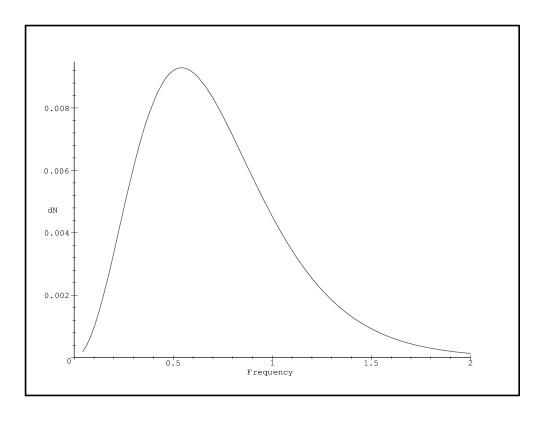
FIG. 3.: Number spectrum (photons per unit volume) for $n_{\mathrm{i}n}=1$, $n_{\mathrm{o}ut}=2$. The horizontal axis is $\omega_{\mathrm{o}ut}$ and is expressed in PHz. The typical timescale $t_{0}$ is set equal to one $fs$. The vertical axis is in arbitrary units.

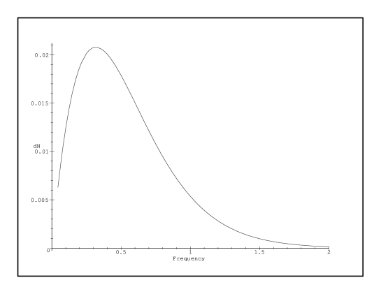
FIG. 4.: Number spectrum for a Planck blackbody curve with $k_{B}T=(n_{\mathrm{i}n}^{2}+n_{\mathrm{o}ut}^{2})/(4\pi t_{0}\;n_{\mathrm{o}ut}\;\hbox{min}\{n_{\mathrm{i}n},n_{\mathrm{o}ut},{\textstyle{1\over 2}}|n_{\mathrm{i}n}-n_{\mathrm{o}ut}|\}).$ The horizontal axis is $\omega_{\mathrm{o}ut}$ and is expressed in PHz. The typical timescale $t_{0}$ is set equal to one fs. The vertical axis is in arbitrary units (but with the same normalization as figure 1).

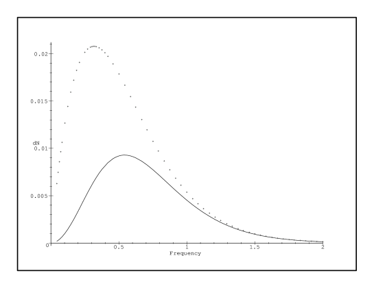
FIG. 5.: Superimposed number spectra (the Planck spectrum is the dotted one). This figure demonstrates the similar high-frequency behaviour although low energy behaviour is different (quadratic versus linear).

F Lessons from this toy model

Lesson 1: This is only a toy model, but we feel it adequately proves that efficient photon production occurs only in the sudden approximation, and that photon production is suppressed in the adiabatic regime. The particular choice of profile $\epsilon(\tau)$ was merely a convenience, it allowed us to get analytic exact results, but it is not a critical part of the analysis. One might worry that the results of this toy model are specific to the choice of profile (37). That the results are more general can be established by analyzing general bounds on the Bogolubov coefficients, which is equivalent to studying general bounds on one-dimensional potential scattering [44]. We shall here quote only the key result that for any monotonic change in the dielectric constant the sudden approximation provides a strict upper bound on the magnitude of the Bogolubov coefficients [44].

Lesson 2: Eberlein’s model for sonoluminescence [20, 21, 22] explicitly uses the adiabatic approximation. For arbitrary adiabatic changes we expect the exponential suppression to still hold with $\rho$ now being some measure of the timescale over which the refractive index changes.

Lesson 3: Schwinger’s model for sonoluminescence [13, 14, 15, 16, 17, 18, 19] implicitly uses the sudden approximation. It is only for the sudden approximation that we recover Schwinger’s phase-space limited spectrum. For arbitrary changes the sudden approximation provides a rigorous upper bound on photon production. It is only in the sudden approximation that efficient conversion of zero-point fluctuations to real photons takes place. Though this result is derived here only for a particularly simple toy model we expect this part of the analysis to be completely generic. We expect that any mechanism for converting zero-point fluctuations to real photons will exhibit similar effects.

G Extensions of this toy model

The major weaknesses of the toy model are that it currently includes neither dispersive effects nor finite volume effects. Including dispersive effects amounts to including condensed matter physics by letting the refractive index itself be a function of frequency. To do this carefully requires a very detailed understanding of the condensed matter physics, which is quite beyond the scope of the present paper. Instead, in this section we shall content ourselves with making order-of-magnitude estimates using Schwinger’s sharp cutoff for the refractive index and the sudden approximation.

The second issue, that of finite volume effects, is addressed more carefully in the companion paper [42]. Finite volume effects are expected to be significant but not overwhelmingly large. From estimates of the available Casimir energy developed in [25], the fractional change in available Casimir energy due to finite volume effects is expected to be of order $1/(KR)=\hbox{(cutoff wavelength)}/(2\pi\hbox{(minimum bubble radius)})$ which is approximately $(300\;\hbox{nm})/(2\pi\;500\;\hbox{nm})\approx 10\%\;$.

Returning to dispersive issues: if the refractive indices were completely non-dispersive (frequency-independent), then the sudden approximation would imply infinite energy production. In the real physical situation $n_{\mathrm{i}n}$ is a function of $\omega_{\mathrm{i}n}$ and $n_{\mathrm{o}ut}$ is a function of $\omega_{\mathrm{o}ut}$. Schwinger’s sharp momentum-space cutoff for the refractive index is equivalent, in this formalism, to the choice

$$n_{\mathrm{i}n}(k)=n_{\mathrm{i}n}\;\Theta(K_{\mathrm{i}n}-k)+1\;\Theta(k-K_{\mathrm{i}n}),$$ (70)

$$n_{\mathrm{o}ut}(k)=n_{\mathrm{o}ut}\;\Theta(K_{\mathrm{o}ut}-k)+1\;\Theta(k-K_{\mathrm{o}ut}),$$ (71)

(More complicated models for the cutoff are of course possible at the cost of obscuring the analytic properties of the model) Although in general the two cutoff wavenumbers, $K_{\mathrm{i}n}$ and $K_{\mathrm{o}ut}$ can be different, it is easy to show (using the delta function and the fact that $\beta\rightarrow 0$ when $n_{\mathrm{i}n}=n_{\mathrm{o}ut}=1$), that this is equivalent to a single common cutoff $K\equiv\hbox{min}\{K_{\mathrm{i}n},K_{\mathrm{o}ut}\}$. From equation (58), taking into account the two photon polarizations, one obtains

$$|\beta(\vec{k}_{\mathrm{i}n},\vec{k}_{\mathrm{o}ut})|^{2} \approx {1\over 2}\frac{\left(n_{\mathrm{o}ut}-n_{\mathrm{i}n}\right)^{2}}{n_{\mathrm{i}n}n_{\mathrm{o}ut}}{V\over(2\pi)^{3}}\;\Theta(K-k_{\mathrm{i}n})\;\Theta(K-k_{\mathrm{o}ut})\;\delta^{3}(\vec{k}_{\mathrm{i}n}+\vec{k}_{\mathrm{o}ut}).$$ (72)

As a consistency check, expression (72) has the desirable property that $\beta\to 0$ as $n_{\mathrm{o}ut}\to n_{\mathrm{i}n}$: That is, if there is no change in the refractive index, there is no particle production. In fact the computed Bogolubov coefficient is directly related to the physical quantities we are interested in

$${dN\over d^{3}\vec{k}_{\mathrm{o}ut}}=\int|\beta(\omega_{\mathrm{i}n},\omega_{\mathrm{o}ut})|^{2}\;d^{3}\vec{k}_{\mathrm{i}n},$$ (73)

$${dN\over dk_{\mathrm{o}ut}}=4\pi k_{\mathrm{o}ut}^{2}\;\int|\beta(\omega_{\mathrm{i}n},\omega_{\mathrm{o}ut})|^{2}\;d^{3}\vec{k}_{\mathrm{i}n},$$ (74)

$${dN\over d\omega_{\mathrm{o}ut}}=4\pi\frac{n_{\mathrm{o}ut}^{3}\omega_{\mathrm{o}ut}^{2}}{c^{3}}\;\int|\beta(\omega_{\mathrm{i}n},\omega_{\mathrm{o}ut})|^{2}\;d^{3}\vec{k}_{\mathrm{i}n},$$ (75)

$$N=\int{dN\over d\omega_{\mathrm{o}ut}}\;d\omega_{\mathrm{o}ut},$$ (76)

and

$$E=\hbar\int{dN(\omega_{\mathrm{o}ut})\over d\omega_{\mathrm{o}ut}}\;\omega_{\mathrm{o}ut}\;d\omega_{\mathrm{o}ut}.$$ (77)

So we can now compute the spectrum, the number, and the total energy of the emitted photons.

$${dN(\omega_{\mathrm{o}ut})\over d\omega_{\mathrm{o}ut}}=\frac{n_{\mathrm{o}ut}}{c}\;{dN(\omega_{\mathrm{o}ut})\over dk_{\mathrm{o}ut}} = \frac{n_{\mathrm{o}ut}}{c}\;4\pi k^{2}_{\mathrm{o}ut}{dN(\omega_{\mathrm{o}ut})\over d^{3}{\vec{k}}_{\mathrm{o}ut}}$$ (78)

$$\approx {n_{\mathrm{o}ut}\over(2\;c)}\;{\left(n_{\mathrm{o}ut}-n_{\mathrm{i}n}\right)^{2}\over n_{\mathrm{o}ut}\,n_{\mathrm{i}n}}{V\over(2\pi)^{3}}\;4\pi\;k_{\mathrm{o}ut}^{2}\;\Theta(K-k_{\mathrm{o}ut})\;$$ (79)

$$= {1\over(2\;c^{3})}\;{n_{\mathrm{o}ut}^{2}}\;{\left(n_{\mathrm{o}ut}-n_{\mathrm{i}n}\right)^{2}\over n_{\mathrm{i}n}}{V\over(2\pi)^{3}}\;4\pi\;\omega_{\mathrm{o}ut}^{2}\;\Theta\left(K-\frac{n_{\mathrm{o}ut}\omega_{\mathrm{o}ut}}{c}\right)$$ (80)

The number of emitted photons is then approximately

$$N \approx {1\over 2}\;{n_{\mathrm{o}ut}^{2}}\;{\left(n_{\mathrm{o}ut}-n_{\mathrm{i}n}\right)^{2}\over n_{\mathrm{i}n}}\;{V\over(2\pi)^{3}}\;{4\pi\over 3}\;(K/n_{\mathrm{o}ut})^{3}$$ (81)

$$= {1\over 12\pi^{2}}\;{\left(n_{\mathrm{o}ut}-n_{\mathrm{i}n}\right)^{2}\over n_{\mathrm{i}n}n_{\mathrm{o}ut}}\;{VK^{3}}.$$ (82)

So that for a spherical bubble

$$N \approx {1\over 9\pi}\;{\left(n_{\mathrm{o}ut}-n_{\mathrm{i}n}\right)^{2}\over n_{\mathrm{o}ut}n_{\mathrm{i}n}}\;(RK)^{3}.$$ (83)

It is important to note that the wavenumber cutoff $K$ appearing in the above formula is not equal to the observed wavenumber cutoff $K_{\mathrm{o}bserved}$. The observed wavenumber cutoff is in fact the upper wavelength measured once the photons have left the bubble and entered the ambient medium (water), so actually

$$K={\omega_{\mathrm{m}ax}n_{\mathrm{o}ut}\over c}={n_{\mathrm{o}ut}\over n_{\mathrm{l}iquid}}\;K_{\mathrm{o}bserved}.$$ (84)

Thus

$$N \approx {1\over 9\pi}\;{\left(n_{\mathrm{o}ut}-n_{\mathrm{i}n}\right)^{2}\over n_{\mathrm{o}ut}n_{\mathrm{i}n}}\;\left(R\;{n_{\mathrm{o}ut}\over n_{\mathrm{l}iquid}}\;K_{\mathrm{o}bserved}\right)^{3}.$$ (85)

$$= {1\over 9\pi}\;{\left(n_{\mathrm{o}ut}-n_{\mathrm{i}n}\right)^{2}\over n_{\mathrm{i}n}}\;n_{\mathrm{o}ut}^{2}\;\left({R\omega_{\mathrm{m}ax}\over c}\right)^{3}.$$ (86)

The total emitted energy is approximately

$$E \approx {1\over 2}\;\frac{n_{\mathrm{o}ut}^{2}}{c^{3}}\;{\left(n_{\mathrm{o}ut}-n_{\mathrm{i}n}\right)^{2}\over n_{\mathrm{i}n}}{V\over(2\pi)^{3}}\;4\pi\;\int\hbar\omega_{\mathrm{o}ut}\;\omega_{\mathrm{o}ut}^{2}\;\Theta\left(K-\frac{n_{\mathrm{o}ut}\omega_{\mathrm{o}ut}}{c}\right)d\omega_{\mathrm{o}ut}$$ (87)

$$= {\hbar\over 2}\;\frac{n_{\mathrm{o}ut}^{2}}{c^{3}}\;{\left(n_{\mathrm{o}ut}-n_{\mathrm{i}n}\right)^{2}\over n_{\mathrm{i}n}}\;{V\over(2\pi)^{3}}\;{4\pi\over 4}\;(K\;c/n_{\mathrm{o}ut})^{4}$$ (88)

$$= {1\over 16\pi^{2}}\;{\left(n_{\mathrm{o}ut}-n_{\mathrm{i}n}\right)^{2}\over n_{\mathrm{i}n}n_{\mathrm{o}ut}^{2}}\;\hbar\;c\;K\;{VK^{3}}$$ (89)

$$= \frac{3}{4}\;N\;\hbar\omega_{\mathrm{m}ax}.$$ (90)

So the average energy per emitted photon is approximately

$$\langle E\rangle={3\over 4}\hbar c\;K/n_{\mathrm{o}ut}={3\over 4}\hbar\;\omega_{\mathrm{m}ax}\sim 3\;{\rm eV}.$$ (91)

Taking into account this extra factor we can now consider some numerical estimates based on our results.

H Some numerical estimates

In Schwinger’s original model he took $n_{\mathrm{g}as}^{\mathrm{i}n}\approx 1$, $n_{\mathrm{g}as}^{\mathrm{o}ut}\approx n_{\mathrm{l}iquid}\approx 1.3$, $V=(4\pi/3)R^{3}$, with $R\approx R_{\mathrm{m}ax}\approx 40\;\mu{\rm m}$ and $K\approx 2\pi/(360\;{\rm nm})$ [16]. Then $KR\approx 698$. Substitution of these numbers into equation (2) leads to an energy budget suitable for about three million emitted photons.

By direct substitution in equation (90) it is easy to check that Schwinger’s results can qualitatively be recovered also in our formalism: in our case we get about 1.8 million photons for the same numbers of Schwinger and about 4 million photons using the updated experimental figures $R_{\mathrm{m}ax}\approx 45\;\mu{\rm m}$ and $K\approx 2\pi/(300\;{\rm nm})$.

A sudden change in refractive index would indeed convert the most of the energy budget based on static Casimir energy calculations into real photons. This may be interpreted as an independent check on Schwinger’s estimate of the Casimir energy of a dielectric sphere. Unfortunately, the sudden (femtosecond) change in refractive index required to get efficient photon production is also the fly in the ointment that kills Schwinger’s original choice of parameters: The collapse from $R_{\mathrm{m}ax}$ to $R_{\mathrm{m}in}$ is known to require approximately $10\;{\rm ns}$, which is far too long a timescale to allow us to adopt the sudden approximation.

In our new version of the model we have $R\approx R_{\mathrm{l}ight-emitting-region}\approx R_{\mathrm{m}in}\approx 500\;\hbox{nm}$ and take $K_{\mathrm{o}bserved}\approx 2\pi/(200\;{\mathrm{n}m})$ so that $K_{\mathrm{o}bserved}R\approx 5\pi\approx 15$. To get about one million photons we now need, for instance, $n_{\mathrm{i}n}\approx 1$ and $n_{\mathrm{o}ut}\approx 12$, or $n_{\mathrm{i}n}\approx 2\times 10^{4}$ and $n_{\mathrm{o}ut}\approx 1$, or even $n_{\mathrm{o}ut}\approx 25$ and $n_{\mathrm{i}n}\approx 71$, though many other possibilities could be envisaged. In particular, the first set of values could correspond to a change of the refractive index at the van der Waals hard core due to a sudden compression e.g., generated by a shock wave. In this framework it is obvious that the most favorable composition for the gas would be a noble gas since this mechanism would be most effective if the gas could be enormously compressed without being easily ionizable.

Note that the estimated values of $n_{\mathrm{g}as}^{\mathrm{o}ut}$ and $n_{\mathrm{g}as}^{\mathrm{i}n}$ are extremely sensitive to the precise choice of cutoff, and the size of the light emitting region, and that the approximations used in taking the infinite volume limit underlying the use of our homogeneous dielectric model are uncontrolled. (The complications attendant on any attempt at including finite volume effects are sufficiently complex as to warrant being relegated to a separate technical paper. [42]) We should not put to much credence in the particular numerical value of $n_{\mathrm{g}as}^{\mathrm{o}ut}$ estimated by these means, but should content ourselves with this qualitative message: We need the refractive index of the contents of the gas bubble to change dramatically and rapidly to generate the photons. Compare this with the calculation and arguments presented by Yablonovitch [34], who points out that ionization processes can and often do cause such sudden drops in the refractive index.

As a final remark we stress that equation (2) and equation (90) are not quite identical. The volume term for photon production that we have just derived [equation (90)] is of second order in $(n_{\mathrm{i}n}-n_{\mathrm{o}ut})$ and not of first order like equation (2). This is ultimately due to the fact that the interaction term responsible for converting the initial energy in photons is a pairwise squeezing operator (see [26]). Equation (90) demonstrates that any argument that attempts to deny the relevance of volume terms to sonoluminescence due to their dependence on $(n_{\mathrm{i}n}-n_{\mathrm{o}ut})$ has to be carefully reassessed. In fact what you measure when the refractive index in a given volume of space changes is not directly the change in the static Casimir energy of the “in” state, but rather the fraction of this static Casimir energy that is converted into photons. We have just seen that once conversion efficiencies are taken into account, the volume dependence is conserved, but not the power in the difference of the refractive index. Indeed the dependence of $|\beta|^{2}$ on $(n_{\mathrm{i}n}-n_{\mathrm{o}ut})^{2}$, and the symmetry of the former under the interchange of “in” and “out” states, also proves that it is the amount of change in the refractive index and not its “direction” that governs particle production. This apparent paradox is easily solved by taking into account that the main source of energy is the acoustic field and that the amount of this energy actually converted in photons during each cycle is a very small fraction of the total acoustic energy.

I Estimating the number of photons

Using the above as a guide to the appropriate starting point, we can now systematically explore the relationship between the in and out refractive indexes and the number of photons produced. Using $K_{\mathrm{o}bserved}R\approx 15$ we get

$$N={119\over n_{\mathrm{l}iquid}^{3}}\;(n_{\mathrm{o}ut}-n_{\mathrm{i}n})^{2}\;{n_{\mathrm{o}ut}^{2}\over n_{\mathrm{i}n}}.$$ (92)

This equation can be algebraically solved for $n_{\mathrm{i}n}$ as a function of $n_{\mathrm{o}ut}$ and $N$. (It’s a quadratic.) For $N=10^{6}$ emitted photons the result is plotted in figure (6). For any specified value of $n_{\mathrm{o}ut}$ there are exactly two values of $n_{\mathrm{i}n}$ that lead to one million emitted photons. To understand the qualitative features of this diagram we consider three sub-regions.

FIG. 6.: The initial refractive index $n_{\mathrm{i}n}$ plotted as a function of $n_{\mathrm{o}ut}$ when one million photons are emitted in the sudden approximation.

First, if $n_{\mathrm{i}n}\ll n_{\mathrm{o}ut}$ then we can approximate

$$n_{\mathrm{i}n}\approx{119\;n_{\mathrm{o}ut}^{4}\over n_{\mathrm{l}iquid}^{3}\;N}.$$ (93)

This corresponds to the region near the origin, and we focus on this region in figure (7).

FIG. 7.: The initial refractive index $n_{\mathrm{i}n}$ plotted as a function of $n_{\mathrm{o}ut}$ when one million photons are emitted in the sudden approximation. Here we focus on the branch that approaches the origin.

Second, if $n_{\mathrm{i}n}\gg n_{\mathrm{o}ut}$ then we can approximate

$$n_{\mathrm{i}n}\approx{n_{\mathrm{l}iquid}^{3}\;N\over 119\;n_{\mathrm{o}ut}^{2}}.$$ (94)

This corresponds to the region near the $y$ axis, and we focus on this region in figure (8).

FIG. 8.: The initial refractive index $n_{\mathrm{i}n}$ plotted as a function of $n_{\mathrm{o}ut}$ when one million photons are emitted in the sudden approximation. Here we focus on the branch that approaches the $y$ axis.

Third, if $n_{\mathrm{i}n}\approx n_{\mathrm{o}ut}$ then we can approximate

$$N\approx{119\over n_{\mathrm{l}iquid}^{3}}\;(n_{\mathrm{i}n}-n_{\mathrm{o}ut})^{2}\;n_{\mathrm{o}ut},$$ (95)

so that

$$n_{\mathrm{i}n}\approx n_{\mathrm{o}ut}\pm\sqrt{N\;n_{\mathrm{l}iquid}^{3}\over 119\;n_{\mathrm{o}ut}}.$$ (96)

This corresponds to the region near the asymptote $n_{\mathrm{i}n}=n_{\mathrm{o}ut}$.

Thus to get a million photons emitted from the van der Waals hard core in the sudden approximation requires a significant (but not enormous) change in refractive index. There are many possibilities consistent with the present model and the experimental data.

IV Experimental features and possible tests

Our proposal shares with other proposals based on the dynamical Casimir effect the main points of strength previously sketched. On the other hand we feel it important to stress that the model we have developed implies a much more complex and rich collection of physical effects due to the fact that photon production from vacuum is no longer due to the simple motion of the bubble boundary. The model indicates that a viable Casimir route to SL cannot avoid a “fierce marriage” with features related to condensed matter physics. As a consequence our proposal is endowed both with general characteristics, coming from its Casimir nature, and with particular ones coming from the details underlying the sudden change in the refractive index.

Although the calculation presented above is just a “probe”, we can see that it is already able to make some general predictions that one can expect to see confirmed in a more complete approach. First of all the photon number spectrum the model predicts is not a black body. It is polynomial at low frequencies ($\omega^{2}$ in the infinite volume approximation of this paper), and in principle this difference can be experimentally detected. (The same qualitative prediction can be found in Schützhold et al. [37].) Moreover the spectrum is expected to be a power law dramatically ending at frequencies corresponding to the physical wave-number cutoff $K$ (at which the refractive indices go to 1). This cutoff implies the absence of hard UV photons and hence, in accordance with experiments, the absence of dissociation phenomena in the water surrounding the bubble.

It is the sudden approximation adopted in this paper that makes it possible to mimic the experimentally observed spectrum. For either a rise in refractive index from $1$ to $12$, or a drop in refractive index from $2\times 10^{4}$ to $1$ one can produce approximately one million photons with frequency mainly in the visible range. The quasi-thermal nature of the emitted photons can be explained by the squeezed nature of the photon pairs that are generically created via dynamical Casimir effect (see reference [26]). Single-photon measurements are then thermal but the core of the bubble is not required to achieve the tremendous physical temperatures envisaged by other models. The apparent temperature measured in single-photon observables can be instead linked to the degree of squeezing of the photon-pairs. As it will be explained in [26], two-photon observables do not exhibit the same thermal statistics, and therefore measurements of suitable two-photon observables provide a useful diagnostic for SL models based on the dynamical Casimir effect. This is a general feature of all models based on photon creation from the QED vacuum and hence it can be used as a definitive test of the presence of a dynamical Casimir effect.

In this type of model, the flash of photons is predicted to occur at the end of the collapse, the scale of emission zone is of the order of $500\;\hbox{nm}$, and the timescale of emission is very short (with a rise-time of the order of femtoseconds, though the flash duration may conceivably be somewhat longer . These are points in substantial agreement with observations. In the infinite volume limit the photons emerge in strictly back-to-back fashion. In contrast, for a finite volume bubble we have shown in [42] that the size of the emitting region constrains the model to low angular momentum for the out states. This is a very sharp prediction that is in principle testable with a suitable experiment devoted to the study of the angular momentum decomposition of the outgoing radiation.

Regarding other experimental dependencies, such as the temperature of the water or the role of noble gases, we can give general arguments but a truly predictive analysis can be done only after focussing on a specific mechanism for changing the refractive index.

For instance, the presence of noble gas is likely to change solubilities of gas in the bubble, and this can vary both bubble dynamics and the sharpness of the boundary. Alternatively, a small percentage of noble gas in air can be very important in the behavior of its dielectric constant at high pressure. Indeed, while small admixtures of noble gas will not significantly alter the zero-frequency refractive index, from the Casimir point of view the behaviour of the refractive index over the entire frequency range up to the cutoff is important.

Finally, the temperature of water can instead affect the dynamics of the bubble boundary by influencing the stability of the bubble, changing either the solubility of air in water or the surface tension of the latter. As observed by Schwinger [13, 14, 15, 16, 17, 18, 19], temperature can also affect the dielectric cutoff, and so temperature dependence of SL is quite natural in Schwinger-like approaches.

V Discussion and Conclusions

The present paper presents calculations of the Bogolubov coefficients relating the two QED vacuum states appropriate to changes in the refractive index of a dielectric bubble. We have verified by explicit computation that photons are produced by rapid changes in the refractive index, and are in agreement with Schwinger in that QED vacuum effects remain a viable candidate for explaining SL. However, some details of the particular model considered in the present paper are somewhat different from that originally envisaged by Schwinger. Based largely on the fact that efficient photon production requires timescales of the order of femtoseconds we were led to consider rapid changes in the refractive index as the gas bubble bounces off the van der Waals hard core. It is important to realize that the speed of sound in the gas bubble can become relativistic at this stage.

A key lesson learned from this paper is that in order that the conversion of zero-point fluctuations to real photons be relevant for sonoluminescence we would want the sudden approximation to hold for photons all the way out to the cutoff ($200\;\hbox{nm}$; corresponding to a period of $0.66\times 10^{-15}\;\hbox{seconds}$). That’s a femtosecond timescale. This implies that if conversion of zero-point fluctuations to real photons is a significant part of the physics of sonoluminescence then the refractive index must be changing significantly on femtosecond timescales. Thus the changes in refractive index cannot be just due to the motion of the bubble wall. (The bubble wall is moving at most at Mach 4 [5], for a $1\;\mu\hbox{m}$ bubble this gives a collapse timescale of $10^{-10}$ seconds, about 100 picoseconds.) In this regard, the comments of Yablonovitch [34] are particularly useful. Yablonovitch points out that, for example, sudden ionization of a gas can lead to substantial changes in the refractive index on the sub-picosecond timescale. Nevertheless we do not necessarily commit ourselves to ionization as being the relevant process in sonoluminescence, and are quite content with any rapid change in refractive index, however generated.

This suggests a slightly different physical model from Schwinger’s original suggestion: Certainly the Casimir energy changes as the bubble collapses, but it is only in the sudden approximation that we can justify converting almost all of the change in Casimir energy to real photons. We thus suggest that one should not be focusing on the actual collapse of the bubble, but rather the way in which the refractive index changes as a function of space and time: As the bubble collapses the gases inside are compressed, and although the refractive index for air (plus noble gas contaminants) is 1 at STP it should be no surprise to see the refractive index of the trapped gas undergoing major changes during the collapse process—especially near the moment of maximum compression when the molecules in the gas bounce off the van der Waals’ hard core repulsive potential.

Thus attempts at using the dynamical Casimir effect to explain SL are now much more tightly constrained than previously. We have shown that any plausible model using the dynamical Casimir effect to explain SL must use the sudden approximation, and must have very rapid changes in the refractive index with a timescale of femtoseconds.

If the light is being emitted only at the core bounce, at $R\approx 500\;{\rm nm}$, then we can get the timescales we want (femtoseconds) without superluminal effects, but we are rather limited in the amount of angular momentum we can get out. Of course, the present model is nowhere near a complete theory: Presently we can relate only the asymptotic “in” states to the asymptotic “out” states via these Bogolubov coefficients. A complete theory of SL will need to address much more specific timing information and this will require a fully dynamical approach (from the QFT point of view) and a deeper understanding (from the condensed matter side) of the precise spatio-temporal dependence of the refractive index as the bubble collapses. In absence of such a more detailed description the present calculation is a useful first step. Moreover it allows us to specify certain basic “signatures” of the effect that may be amenable to experimental test. To this end we have developed use of two-photon statistics as a diagnostic for the dynamical Casimir effect [26]. In this paper we have addressed the basic physical scenario; all technical complications due to finite volume effects are relegated to a companion paper [42]. We feel that, as an explanation for sonoluminescence, we have now driven models based on the dynamical Casimir effect into a relatively small region of parameter space, and are hopeful of experimental verification (or falsification) in the not too distant future.

Stripped to its fundamentals, we therefore view the Schwinger mechanism as this: Bubble collapse leads to changes in the spatio-temporal distribution of the refractive index, both via physical movement of the dielectrics, and through the time-dependent properties of the dielectrics. Changes in the refractive index drive changes in the distribution of zero-point modes, and this change in zero-point modes is reflected in real photon production.

In light of these observations we think that one can also derive a general conclusion about the long-standing debate on the actual value of the static Casimir energy and its relevance to sonoluminescence: Sonoluminescence cannot be directly related to the static Casimir effect. (The static Casimir effect is relevant only insofar as it gives an approximate value for the energy budget). We hope that the investigation of this paper will convince everyone that only models dealing with the actual mechanism of particle creation (a mechanism which must have the qualities we have discussed) will be able to eventually prove or disprove the pertinence of the physics of the quantum vacuum to Sonoluminescence. This implies that continuing debate about the static Casimir effect can be now seen as marginal and irrelevant with respect to the real physical problems of SL.

In conclusion the present calculation (limited though it may be) represents an important advance: There now can be no doubt that changes of the refractive index of the gas inside the bubble lead to production of real photons—the controversial issues now move to quantitative ones of precise fitting of the observed experimental data. We are hopeful that more detailed models and data fitting will provide better explanations of the details of the SL effect, and specifically wish to assert that models based on the QED vacuum remain viable.

REFERENCES

- [1] E-mail: liberati@sissa.it
- [2] E-mail: visser@kiwi.wustl.edu
- [3] E-mail: belgiorno@mi.infn.it
- [4] E-mail: sciama@sissa.it
- [5] B.P. Barber, R.A. Hiller, R. Löfstedt, S.J. Putterman Phys. Rep. 281, 65-143 (1997).
- [6] B. Gompf, R. Günther, G. Nick, R. Pecha, and W. Eisenmenger, Phys. Rev. Lett. 78, 1405 (1997).
- [7] R.A. Hiller, S.J. Putterman, and K.R. Weninger, Phys. Rev. Lett. 80, 1090 (1998).
- [8] D. Lohse and S. Hilgenfeldt, J. Chem. Phys. 107 (1997), 6986.
-
[9]
T.J. Matula and L.A. Crum,
Phys. Rev. Lett. 80, 865 (1998).
J.A. Ketterling and R.E. Apfel Phys. Rev. Lett. 81, 4991 (1998). - [10] J.B. Young, T. Schmiedel, Woowon Kang Phys. Rev. Lett. 77, 4816 (1996).
- [11] B.A. DiDonna, T.A. Witten, J.B. Young, Physica A 258, 263 (1998).
- [12] S. Hilgenfeldt, D. Lohse, and W.C. Moss, Phys. Rev. Lett. 80, 1332 (1998).
- [13] J. Schwinger, Proc. Nat. Acad. Sci. 89, 4091–4093 (1992).
- [14] J. Schwinger, Proc. Nat. Acad. Sci. 89, 11118–11120 (1992).
- [15] J. Schwinger, Proc. Nat. Acad. Sci. 90, 958–959 (1993).
- [16] J. Schwinger, Proc. Nat. Acad. Sci. 90, 2105–2106 (1993).
- [17] J. Schwinger, Proc. Nat. Acad. Sci. 90, 4505–4507 (1993).
- [18] J. Schwinger, Proc. Nat. Acad. Sci. 90, 7285–7287 (1993).
- [19] J. Schwinger, Proc. Nat. Acad. Sci. 91, 6473–6475 (1994).
- [20] C. Eberlein, Sonoluminescence as quantum vacuum radiation, Phys. Rev. Lett. 76, 3842 (1996). quant-ph 9506023
- [21] C. Eberlein, Theory of quantum radiation observed as sonoluminescence, Phys. Rev. A 53, 2772 (1996). quant-ph 9506024
- [22] C. Eberlein, Sonoluminescence as quantum vacuum radiation (reply to comment), Phys. Rev. Lett. 78, 2269 (1997). quant-ph/9610034
- [23] C. E. Carlson, C. Molina–París, J. Pérez–Mercader, and M. Visser, Phys. Lett. B 395, 76-82 (1997). hep-th/9609195
- [24] C. E. Carlson, C. Molina–París, J. Pérez–Mercader, and M. Visser, Phys. Rev. D56, 1262 (1997). hep-th/9702007.
- [25] C. Molina–París and M. Visser, Phys. Rev. D56, 6629 (1997). hep-th/9707073
- [26] F. Belgiorno, S. Liberati, M. Visser, and D.W. Sciama, Sonoluminescence: two-photon correlations as a test for thermality, to appear.
- [27] K. Milton, Casimir energy for a spherical cavity in a dielectric: toward a model for Sonoluminescence?, in Quantum field theory under the influence of external conditions, edited by M. Bordag, (Tuebner Verlagsgesellschaft, Stuttgart, 1996), pages 13–23. See also hep-th/9510091.
- [28] K. Milton and J. Ng, Casimir energy for a spherical cavity in a dielectric: Applications to Sonoluminescence, Phys. Rev. E55 (1997) 4207; hep-th/9607186.
- [29] K. Milton and J. Ng, Observability of the bulk Casimir effect: Can the dynamical Casimir effect be relevant to Sonoluminescence?, Phys. Rev. E57 (1998) 5504; hep-th/9707122.
- [30] K. Milton, V.N. Marchevsky, and I. Brevik, Identity of the van der Waals force and the Casimir effect and the irrelevance of these phenomena to sonoluminescence, hep-th/9810062.
- [31] P. Candelas, Ann. of Phys. 167, 57-84 (1986)
- [32] I.H. Brevik, V.V. Nesterenko, and I.G. Pirozhenko, Direct mode summation for the Casimir energy of a solid ball, hep-th/9710101.
- [33] V.V. Nesterenko and I.G. Pirozhenko, Is the Casimir effect relevant to sonoluminescence?, hep-th/9803105.
- [34] E. Yablonovitch, Phys. Rev. Lett. 62, 1742 (1989)
-
[35]
C.S. Unnikrishnan and S. Mukhopadhyay,
Phys. Rev. Lett. 77, 4960 (1996).
A. Lambrecht, M-T. Jaekel, and S. Reynaud, Phys. Rev. Lett. 78, 2267 (1997).
N. García and A.P. Levanyuk, Phys. Rev. Lett. 78, 2268 (1997). - [36] M. Jackel and S. Reynaud, Quantum Opt. 4, 39 (1992)
- [37] R. Schützhold, G. Plunien, and G. Soff, Quantum radiation in external background fields, Phys. Rev. A58, 1783 (1998). quant-ph/9801035.
- [38] J. Holzfuss, M. Rüggeberg, and A. Billo, Phys. Rev. Lett. 81, 5434 (1998).
- [39] C.C. Wu and P.H. Roberts, Proc. R. Soc. Lond. A445, 323 (1994); is found on page 325, line 3 from bottom.
- [40] S. Hilgenfeldt, M.P. Brenner, S. Grossmann and D. Lohse, J. Fluid. Mech. 365 (1998), 171.
- [41] W.C. Moss, D.B. Clarke, J.W. White, and D.A. Young, Phys. Fluids. 6 (1994) 2979.
- [42] S. Liberati, M. Visser, F. Belgiorno, and D.W. Sciama, Sonoluminescence as a QED vacuum effect. II: Finite Volume Effects, to appear.
- [43] N.D. Birrell and P.C.W. Davies, Quantum fields in curved space, (Cambridge University Press, Cambridge, England, 1982).
- [44] M. Visser, Some general bounds for 1-D scattering, Phys. Rev. A59 (1999) 427–438.