Quantum computing with neutral atoms

Abstract

We develop a method to entangle neutral atoms using cold controlled collisions. We analyze this method in two particular set-ups: optical lattices and magnetic micro-traps. Both offer the possibility of performing certain multi-particle operations in parallel. Using this fact, we show how to implement efficient quantum error correction and schemes for fault-tolerant computing.

I Introduction

Entanglement is one of the most intriguing features of Quantum Mechanics. However, there are very few physical systems in which entanglement can be systematically studied in a controlled way. Those systems include ion-traps [1, 2, 3, 4, 5, 6, 7, 8], cavity QED [9, 10, 11, 12, 13, 14, 15, 16], photons [17, 18, 19, 20, 21, 22, 23, 24, 25], and molecules in the context of NMR [26, 27, 28, 29] (see [30] however). Very recently, we have identified a new way of entangling particles by using cold controlled collisions with which one could study experimentally basic issues of quantum information theory [31]. Given the impressive experimental advances made so far in the fields of neutral atom trapping and cooling [32, 33, 34, 35], and in the studies of Bose Einstein condensation (BEC) of ultracold gases [36, 37, 38, 39, 40, 41], that proposal opens a new perspective to several experimental groups who so far have concentrated their efforts in other fields of Atomic Physics.

In the present paper, we build upon the work in [31] and explore the idea of using atomic controlled cold collisions for entangling neutral atoms in optical lattices (see also [42]) and in arrays of magnetic micro-traps. We show how to perform two-qubit gate operations with those systems obtaining very high fidelities. We propose a variety of experiments to entangle particles using state-of-the-art technology. We also concentrate on the unique possibilities that these set-ups offer to perform multi-particle entanglement operations in parallel [43, 44, 45, 46]. Using such parallelism, we show how to implement efficient error correction [47, 48, 49, 50, 51, 52, 53, 54] and fault-tolerant quantum computation schemes [55, 56, 57, 58, 59, 60, 61, 62].

The paper is organized as follows. In Sec. II we discuss the use of ultracold collisions as a mechanism for entangling neutral atoms. Such collisions can be brought about by either moving the potentials in certain spatial directions or by modifying the shape of the trapping potentials. In Sec. III we describe two systems in which such operations can be implemented. These are optical lattices [42, 63, 64, 65, 66] and magnetic microtraps [67, 68, 69, 70, 71] both of which have been studied experimentally in detail in the past. In Sec. IV we describe a class of multi-particle entanglement operations that can be realized in these systems (we concentrate here on optical lattices). The usefulness of such operations for quantum computing depends on certain conditions that need to be satisfied in an experiment. Among these conditions, the filling problem, i.e. how to fill the potentials with regular patterns of atoms, is most outstanding. We discuss these matters and show that even under present-day experimental conditions, very interesting entanglement studies could be performed. Section V summarizes the main results and discusses their relevance for future research.

II Entanglement of atoms via cold controlled collisions

In this Section, we consider two bosonic neutral atoms with two internal states trapped by conservative potentials and cooled to the motional ground states. Initially these two particles are sufficiently far apart so that they do not interact with each other. We then assume the shape of the potentials to be varied in a way that depends on the internal state of the atoms so that the two particles come close to each other if they are in certain internal states. As we will show, this can be done e.g. by moving the center position of the trapping potentials state selectively, or by switching off a potential barrier between the two atoms for one of the two internal states. In both cases the particles will interact via $s$-wave scattering with each other in a coherent way when they are close to each other. After the interaction has taken place the particles are restored to their initial position. In this way one can implement conditional dynamics and realize a fundamental two-qubit gate.

Note that we are dealing with bosons. Therefore, we have to use symmetrized wave functions for describing the two particles. It will turn out that if the center positions of the trapping potentials are moved state selectively, particles in the same internal state will always be so far apart that their wave functions never overlap. Thus, we will not care about the symmetrization in this case. On the other hand, if the potential barrier is switched off for one internal state, particles in the same internal state will come close to each other and symmetrizing the wave function is essential.

A Hamiltonian

Here we deal with the interaction Hamiltonian of two neutral atoms $1$ and $2$ with internal states $|a\rangle_{1,2}$ and $|b\rangle_{1,2}$ trapped by conservative potentials $V^{\beta_{i}}({\bf x}_{i},t)$ whose functional dependence on the coordinate ${\bf x}_{i}$, with $i=1,2$ the particle index, depends on the internal state of the particle $\beta_{1,2}=a,b$. Initially, the two particles are in the ground state of the trapping potentials and the centers of the two potential wells are sufficiently far apart so that the particles do not interact. Then the form of the potential wells is changed such that there is some overlap of the wave functions of the two atoms, and the particles will interact with each other. This interaction between the atoms in two given internal states $\beta_{1}$ and $\beta_{2}$ can be described by a contact potential

$$u^{\beta_{1}\beta_{2}}({\bf x}_{1}-{\bf x}_{2})=\frac{4\pi a_{s}^{\beta_{1}\beta_{2}}\hbar^{2}}{m}\delta^{3}({\bf x}_{1}-{\bf x}_{2}),$$ (1)

where $a_{s}^{\beta_{1}\beta_{2}}$ is the $s$-wave scattering length for the corresponding internal states describing elastic collisions and $m$ is the mass of the particles. This zero energy $s$-wave scattering approximation will be valid as long as we assume that $v_{\rm osc}$, the rms velocity of the atoms in the vibrational ground state, approximately given by $v_{\rm osc}\approx a_{0}\omega$, is sufficiently small [72]. Here $a_{0}$ is the size of the ground state of the trap potential, and $\omega$ is the first excitation frequency. Thus we can describe the evolution of the system by the Hamiltonian

$$H=\sum_{\beta_{1},\beta_{2}}H^{\beta_{1}\beta_{2}}\otimes|\beta_{1}\rangle_{1}\langle\beta_{1}|\otimes|\beta_{2}\rangle_{2}\langle\beta_{2}|,$$ (2)

where

$$H^{\beta_{1}\beta_{2}}=\sum_{i=1,2}\left[\frac{({\bf p}_{i})^{2}}{2m}+V^{\beta_{i}}\left({\bf x}_{i},t\right)\right]+u^{\beta_{1}\beta_{2}}({\bf x}_{1}-{\bf x}_{2}).$$ (3)

Here ${\bf p}_{i}$ is the momentum operator.

1 Interaction in perturbation theory

We want to treat the interaction term in the Hamiltonian Eq. (3) perturbatively. For particles in two different internal states $\beta_{1}\neq\beta_{2}$ we find the correction to the energy due to the interaction as

$$\Delta E^{\beta_{1}\beta_{2}}(t)=\frac{4\pi a^{ab}_{s}\hbar^{2}}{m}\int d{\bf x}\prod_{i}\left|\psi^{\beta_{i}}_{i}\left({\bf x},t\right)\right|^{2},$$ (4)

where $\psi^{\beta_{i}}_{i}\left({\bf x},t\right)$ is the normalized one-particle wave function of particle $i$ in internal state $\beta_{i}$ in the time dependent potential $V^{\beta_{i}}\left({\bf x},t\right)$. If the particles are in the same internal state $\beta_{1}=\beta_{2}=\beta$, we have to account for the Bose statistics i.e. use the properly normalized symmetrized two-particle wave function for calculating the energy shift. We therefore find

$$\Delta E^{\beta\beta}(t)=\frac{8\pi a^{\beta\beta}_{s}\hbar^{2}}{m(1+|\alpha|^{2})}\int dx\prod_{i}\left|\psi^{\beta}_{i}\left({\bf x},t\right)\right|^{2},$$ (5)

where

$$\alpha=\int dx\left(\psi^{\beta}_{1}\left({\bf x},t\right)\right)^{*}\psi^{\beta}_{2}\left({\bf x},t\right).$$ (6)

For general $\beta_{1}$, $\beta_{2}$ we find the phase accumulated due to the interaction in the time interval $[-\tau,\tau]$ by

$$\phi^{\beta_{1}\beta_{2}}=\frac{1}{\hbar}\int_{-\tau}^{\tau}\!dt\,\Delta E^{\beta_{1}\beta_{2}}(t).$$ (7)

B Moving potentials

One way of controlling the interaction between the particles is to move the center position of the potentials $V^{\beta_{i}}\left({\bf x}_{i},t\right)=V\left({\bf x}_{i}-\bar{\bf x}_{i}^{\beta_{i}}(t)\right)$ towards each other in a state-dependent way while leaving the shape of the potential unchanged. By moving the potential we get two kinds of phase shifts. A kinetic phase which is a single-particle phase due to the kinetic energy of the particles and an interaction phase due to coherent interactions between two atoms. First we will define these two phases for general trapping potentials and afterwards specialize them to moving harmonic potentials. Finally, we will show how conditional dynamics can be realized.

1 Kinetic phase

First we want to consider a single atom in internal state $|\beta\rangle$ trapped in the instantaneous ground state $\psi_{0}$ of a moving potential well $V({\bf x}-\bar{\bf x}^{\beta}(t))$. The center position of the potential is moved along a trajectory $\bar{\bf x}^{\beta}(t)$. Ideally, we want the atom to remain in the ground state of its trapping potential and to preserve its internal state during the motion. This corresponds to the transformation from $t=-\tau$ to $t=\tau$

$$\psi_{0}[{\bf x}-\bar{\bf x}^{\beta}(-\tau)]\rightarrow e^{-i\phi^{\beta}}\psi_{0}[{\bf x}-\bar{\bf x}^{\beta}(\tau)],$$ (8)

where the atom remains in the ground state of the trapping potential and preserves its internal state. Transformation (8) can be realized in the adiabatic limit [73], where we move the potentials so that the atoms remain in the instantaneous motional ground state. Adiabaticity requires $|\dot{\bar{\bf x}}^{\beta}(t)|\ll v_{\rm osc}$ for all times $t$. The phase $\phi^{\beta}$ can be easily calculated in the limit $|\ddot{\bar{\bf x}}^{\beta}(t)|\ll v_{\rm osc}/\tau$. We find the kinetic phase

$$\phi^{\beta}=\frac{m}{2\hbar}\int_{-\tau}^{\tau}\!dt\,\left(\dot{\bar{\bf x}}^{\beta}(t)\right)^{2}.$$ (9)

2 Interaction phase

Let us now consider two particles $i=1,2$ in different internal states $|\beta_{i}\rangle_{i}$ trapped in the ground states of two moving potentials. Initially, at time $t=-\tau$, these wells are centered at positions $\bar{\bf x}_{i}$, sufficiently far apart (distance $d=\bar{\bf x}_{1}-\bar{\bf x}_{2}$) so that the particles do not interact. The positions of the potentials are moved along trajectories $\bar{\bf x}^{\beta_{i}}_{i}(t)$ so that the wave packets of the atoms overlap for certain time, until finally they are restored to the initial position at the time $t=\tau$. We assume that: (i) $|\dot{\bar{\bf x}}^{\beta_{i}}_{i}(t)|\ll v_{\rm osc}$ (adiabatic condition) so that the particles remain in the ground states of the moving trapping potentials; (ii) The interaction can be treated perturbatively, where $|\Delta E^{\beta_{1}\beta_{2}}(t)|\ll\hbar\omega$ so that no sloshing motion is excited. In that case, we realize the transformation

$$\psi_{0}({\bf x}_{1}-\bar{\bf x}_{1})\psi_{0}({\bf x}_{2}-\bar{\bf x}_{2})\rightarrow$$ (10)

$$\qquad e^{-i\phi}\psi_{0}({\bf x}_{1}-\bar{\bf x}_{1})\psi_{0}({\bf x}_{2}-\bar{\bf x}_{2}),$$ (11)

where $\phi=\phi^{\beta_{1}}+\phi^{\beta_{2}}+\phi^{\beta_{1}\beta_{2}}$ with the collisional phase $\phi^{\beta_{1}\beta_{2}}$ defined in Eq. (7).

3 Moving harmonic potentials

Here we specialize to harmonic trapping potentials. The wave function $\psi^{\beta_{i}}_{i}({\bf x},t)$ of a particle in a moving harmonic potential can be found analytically. In the Appendix A we show that when we start to move the harmonic potential at time $-\tau$ with the particle in its motional ground state and stop to move the potential at time $\tau$, the condition for the particle to end up in the motional ground state at $\tau$ is given by

$$\left|\int_{-\tau}^{\tau}\dot{\bar{\bf x}}^{\beta_{i}}_{i}(t^{\prime})e^{i\omega t^{\prime}}dt^{\prime}\right|\ll a_{0}.$$ (12)

This condition is weaker than the condition $|\dot{\bar{\bf x}}^{\beta_{i}}_{i}(t)|\ll v_{\rm osc}$ for adiabaticity, and means that the particle need not be in the instantaneous ground state of the moving potential at all times, but only at the final time. The kinetic phases can be found exactly (cf. Eq. (A7)). If $|\Delta E^{\beta_{1}\beta_{2}}(t)|\ll\hbar\omega$ is satisfied, the interaction phase can be found by Eq. (7) since the $\psi^{\beta_{i}}_{i}\left({\bf x},t\right)$ are known. It is also possible to generalize these results to the case in which the trap frequency changes with time [74].

4 Implementation of conditional dynamics

Let us now assume that we can design the potentials such that atoms in the internal state $|\beta_{i}\rangle_{i}$ experience a potential $V^{\beta_{i}}({\bf x}_{i},t)=V({\bf x}_{i}-\bar{\bf x}^{\beta_{i}}_{i}(t))$ which is initially ($t=-\tau$) centered at position $\bar{\bf x}_{i}$. We assume that we can move the centers of the potentials as follows: $\bar{\bf x}^{\beta_{i}}_{i}(t)=\bar{\bf x}_{i}+\delta{\bf x}^{\beta_{i}}(t)$. As shown in Fig. 1 the trajectories $\delta{\bf x}^{\beta_{i}}(t)$ are chosen in such a way that $\delta{\bf x}^{\beta_{i}}(-\tau)=\delta{\bf x}^{\beta_{i}}(\tau)=0$ and the first atom collides with the second one only if they are in states $|a\rangle$ and $|b\rangle$, respectively ($|\bar{\bf x}_{1}^{b}(t)-\bar{\bf x}_{2}^{a}(t)|\gg a_{0}$ $\forall t$). This choice is motivated by the physical implementation considered in Sec. III A. The fact that $\bar{\bf x}_{i}$ does not depend on the internal atomic state and the shape of the two potentials is the same at times $\pm\tau$ allows one to easily change the internal state at times $t=\pm\tau$ by applying laser pulses. If the conditions stated above are fulfilled, depending on the initial internal atomic states we have:

$$|a\rangle_{1}|a\rangle_{2} \rightarrow e^{-i2\phi^{a}}|a\rangle_{1}|a\rangle_{2},$$ (13)

$$|a\rangle_{1}|b\rangle_{2} \rightarrow e^{-i(\phi^{a}+\phi^{b}+\phi^{ab})}|a\rangle_{1}|b\rangle_{2},$$ (14)

$$|b\rangle_{1}|a\rangle_{2} \rightarrow e^{-i(\phi^{a}+\phi^{b})}|b\rangle_{1}|a\rangle_{2},$$ (15)

$$|b\rangle_{1}|b\rangle_{2} \rightarrow e^{-i2\phi^{b}}|b\rangle_{1}|b\rangle_{2},$$ (16)

where the motional states remain unchanged. The kinetic phases $\phi^{\beta}$ and the collisional phase $\phi^{ab}$ can be calculated as stated above. We emphasize that the $\phi^{\beta}$ are (trivial) one-particle phases that, as long as they are known, can always be incorporated in the definition of the states $|a\rangle$ and $|b\rangle$. This realizes a fundamental two-qubit quantum gate for certain values of $\phi^{ab}$, e.g. $\phi^{ab}=\pi$.

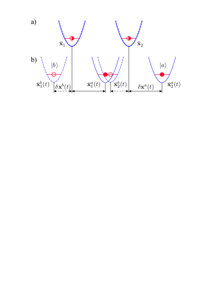
FIG. 1.: Configurations at times $\pm\tau$ (a) and at $t$ (b). The solid (dashed) curves show the potentials for particles in the internal state $|a\rangle$ ($|b\rangle$). Center positions $\bar{\bf x}^{\beta_{i}}_{i}(t)$ and displacements $\delta{\bf x}^{\beta_{i}}(t)$ as defined in the text.

C Switching potentials

The interaction between the particles can be controlled also in another way, for example by changing with time the shape of the potentials depending on the particles’ internal states. Different regimes for the time-dependence of the potential are possible. The two limits of extremely slow (adiabatic) or extremely fast (sudden) potential changes are both interesting and lead to peculiar schemes. Here we will analyze the latter case. We consider two atoms initially trapped in two displaced wells. At a certain time the barrier between the wells is suddenly removed in a selective way for atoms in state $|b\rangle$, whereas it remains unchanged for atoms in state $|a\rangle$. The atoms are allowed to oscillate for some time, and then the barrier is raised again suddenly such as to trap them back at the original positions. During the process they will acquire both a kinematic phase due to the oscillations within their respective wells, and an interaction phase due to the collision. We will calculate such quantities and look for the optimal switching time required in order to maximize the fidelity for a quantum gate relying on this scheme, which we will estimate quantitatively for the relevant physical example in Sec. III B.

1 Kinematic phase

Let us first consider the time-independent problem of an atom subject to a three-dimensional potential whose functional form along $x$ depends on the internal atomic state $\beta=a,b$:

$$V^{\beta}({\bf x})=v^{\beta}(x)+v_{\perp}(y)+v_{\perp}(z).$$ (17)

Here the $v$’s are single-well trapping potentials, and $v^{a}$, $v^{b}$ are centered around $x=x_{0}$, $x=0$, respectively. We assume that the atom is initially prepared in the motional state $|\Psi_{+}\rangle$, where

$$\langle{\bf x}|\Psi_{+}\rangle\equiv\Psi_{+}({\bf x})=\psi_{+}(x)\psi_{\perp}(y)\psi_{\perp}(z)$$ (18)

and $\psi_{+}$, $\psi_{\perp}$ are the ground-state wave functions of $v^{a}$, $v_{\perp}$ with eigenvalues $E^{a}$, $E_{\perp}$ respectively. Thus $\Psi_{+}({\bf x})$ is peaked around the position ${\bf x}_{0}\equiv(x_{0},0,0)$, coinciding with the center of $V^{a}({\bf x})$ but displaced from the one of $V^{b}({\bf x})$. Therefore, if the atom is in internal state $|a\rangle$, its motional state after a time $t$ will be unchanged up to a phase $\phi^{a}=(E^{a}+2E_{\perp})t/\hbar$. If it is instead in state $|b\rangle$, it will start oscillating within the well, thus picking up a different phase $\phi^{b}$ due to the kinematical evolution, and possibly coming back at the initial position after some time.

2 Interaction phase

We now consider two atoms 1 and 2 initially (at $t=0$) prepared in the motional states $|\Psi_{+}\rangle$ and $|\Psi_{-}\rangle$, the latter being defined as in Eq. (18) but with $\psi_{-}(x)\equiv\psi_{+}(-x)$ replacing $\psi_{+}(x)$. We assume that the particles are subject to the potentials $\sum_{\varsigma=+,-}\Theta(\varsigma x)V^{\beta_{i}}(\varsigma{\bf x}_{i})$, where $\Theta$ denotes the step function. If any one of them is in state $|b\rangle$, for $t>0$ it will start oscillating within the well, eventually interacting with the other one. If $v_{\perp}$ is much steeper than $v^{\beta}$, then the probability of transversal excitations can be neglected, i.e. each atom remains in the ground state along $y$ and $z$. By integrating over these variables, the problem is then reduced to a one-dimensional two-particle Schrödinger equation, with

$${\cal H}^{\beta_{1}\beta_{2}}=\sum_{i=1}^{2}\left[\frac{(p_{i})^{2}}{2m}+w^{\beta_{i}}(x_{i},t)\right]+u^{\beta_{1}\beta_{2}}_{x}(x_{1}-x_{2})$$ (19)

replacing the Hamiltonian (3) in Eq. (2). Here $w^{\beta}(x,t)$ is a combination of the $v^{\beta}(x)$ whose form changes with time, and $u^{\beta_{1}\beta_{2}}_{x}$ is an effective interaction potential taking into account the integration over $y$ and $z$, and therefore depending on the shape of $v_{\perp}$. We shall study the dynamics at $t\geq 0$ for different values of $(\beta_{1},\beta_{2})$ separately. If $\beta_{1}=\beta_{2}\equiv\beta$ the total initial normalized state, symmetric under particle interchange, is

$$|\psi^{\beta\beta}(0)\rangle\approx\frac{|\psi_{+}\rangle_{1}|\psi_{-}\rangle_{2}+|\psi_{-}\rangle_{1}|\psi_{+}\rangle_{2}}{\sqrt{2}}\otimes|\beta\rangle_{1}\otimes|\beta\rangle_{2},$$ (20)

where the initial overlap $\langle\psi_{-}|\psi_{+}\rangle\ll 1$ has been neglected in computing the normalization. If both particles are in state $\left|a\right\rangle$, no interaction takes place and thus the collisional phase $\phi^{aa}=0$. Therefore, we shall now consider in more detail the situation in which both particles are in state $\left|b\right\rangle$ and thus move within the well $v^{b}$. In the absence of interaction, after an oscillation period $T$ they would come back exactly to the initial state. Due to the interaction, two effects arise: an additional phase, which is accumulated by the wave function as the number of undergone oscillations increases; and a slight decrease in their frequency, because the atoms acquire a small delay in their motion inside the trap as they come out from a collision. These effects have to be evaluated in detail, since they influence the attainable fidelity for a quantum gate based on this scheme. For symmetry reasons, the relative coordinate motion decouples from the center of mass motion, which is not affected by the interaction and can be solved analytically. For an explicit calculation, it is now needed to specify the form of the potentials in Eq. (17).

3 Switching harmonic potentials

In order to perform the calculations analytically, the potentials in Eq. (17) are chosen to be harmonic:

$$v^{a}(x) = \frac{m\omega_{0}^{2}}{2}(x-x_{0})^{2},$$ (22)

$$v^{b}(x) = \frac{m\omega^{2}}{2}x^{2},$$ (23)

$$v_{\perp}(y) = \frac{m\omega_{\perp}^{2}}{2}y^{2},$$ (24)

where $\omega_{\perp}\gg\omega_{0}>\omega$. Our scheme for gate operation is as follows: initially the two particles are separately stored in two displaced harmonic wells at $\pm x_{0}$ as described above, i.e. with the potential (Fig. 2a)

$$w^{a}(x,t<0) = \sum_{\varsigma=+,-}\Theta(\varsigma x)v^{a}(\varsigma x),$$ (26)

$$w^{b}(x,t<0) = w^{a}(x,t<0)$$ (27)

in the one-dimensional Hamiltonian Eq. (19). At $t=0$ the potential undergoes a sudden change, namely the barrier between the two wells is selectively switched off for state $|b\rangle$ only (Fig. 2b):

$$w^{a}(x,0<t<\tau) = w^{a}(x,t<0);$$ (29)

$$w^{b}(x,0<t<\tau) = v^{b}(x).$$ (30)

Then at $t=\tau$, the potential barrier is suddenly restored: $w^{a,b}(x,t>\tau)=w^{a,b}(x,t<0)$. The time evolution at $0<t<\tau$ is characterized by oscillations with periodicity $T\equiv 2\pi/\omega$. The projection of the evolved CM wave function on the initial one

$$\left|\left\langle\psi^{bb}_{\rm CM}(t)\right|\left.\psi^{bb}_{{\rm CM}}(0)\right\rangle\right|^{2}=\left[1+\frac{\left(\omega_{0}^{2}-\omega^{2}\right)^{2}}{4\omega_{0}^{2}\omega^{2}}\sin^{2}\left(\omega t\right)\right]^{-\frac{1}{2}}$$ (31)

has instead a period of $T/2$, because of the parity of the spatial wave function. The time-dependent energy shift (4) due to the interaction turns out to be

$$\Delta E^{bb}(t)=a_{s}^{bb}\hbar\omega_{\perp}\sqrt{\frac{8m\Omega(t)}{\pi\hbar}}e^{-\frac{2m\omega_{0}}{\hbar}x_{0}^{2}\left[1-\sin^{2}(\omega t)\frac{\omega_{0}\Omega(t)}{\omega^{2}}\right]}\;,$$ (32)

where $\Omega(t)=\omega^{2}\omega_{0}/[\omega^{2}\cos^{2}(\omega t)+\omega_{0}^{2}\sin^{2}(\omega t)]$. Hence the interaction-induced phase shift (7) accumulated after each oscillation period $T$ is (evaluating the integral in a saddle-point approximation)

$$\phi^{bb}_{T} = \int_{0}^{T}\frac{\Delta E^{bb}(t)}{\hbar}dt$$ (33)

$$\approx 8a_{s}^{bb}\sqrt{\frac{m\omega_{0}}{\hbar}\frac{\omega_{y}\omega_{z}}{\omega_{0}^{2}+\omega^{2}(4x_{0}^{2}\,m\omega_{0}/\hbar-1)}}\;.$$ (34)

If the particles are in different internal states, the center of mass does not decouple from the relative motion. No analytical solution is found in this case, and one must resort to numerical techniques to evaluate the collisional phase $\phi^{ab}$.

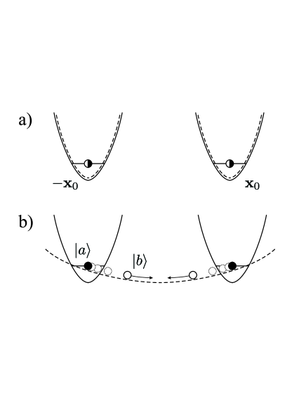
FIG. 2.: Configuration at times $t<0$, $t>\tau$ (a) and at $0\leq t\leq\tau$ (b). The solid (dashed) curves show the potentials for particles in the internal state $|a\rangle$ ($|b\rangle$).

4 Implementation of conditional dynamics

If at time $\tau$ the atoms have come back to their initial spatial distribution, corresponding to a symmetrized product of the ground states of the two wells, then after the barrier is raised they will remain trapped around the original position. The only change in the overall state will be a phase $\phi^{\beta_{1}}_{\tau}+\phi^{\beta_{2}}_{\tau}+\phi^{\beta_{1}\beta_{2}}_{\tau}$ as discussed in Sect. II B 2. Therefore, the gate operation time $\tau$ has to be chosen in such a way as to maximize the overlap $|\langle\psi^{\beta_{1}\beta_{2}}(\tau)|\psi^{\beta_{1}\beta_{2}}(0)\rangle|^{2}$ for all $\beta_{1},\beta_{2}$. If the modifications in the atomic motion due to interaction are not too strong, this condition will be satisfied to a good approximation after an integer number $n$ of oscillations. Thus, for $\tau\approx nT$, the following mapping is realized:

$$|a\rangle_{1}|a\rangle_{2} \rightarrow e^{-i(2\phi^{a}_{\tau}+\phi^{aa}_{\tau})}|a\rangle_{1}|a\rangle_{2},$$ (35)

$$|a\rangle_{1}|b\rangle_{2} \rightarrow e^{-i(\phi^{a}_{\tau}+\phi^{b}_{\tau}+\phi^{ab}_{\tau})}|a\rangle_{1}|b\rangle_{2},$$ (36)

$$|b\rangle_{1}|a\rangle_{2} \rightarrow e^{-i(\phi^{b}_{\tau}+\phi^{a}_{\tau}+\phi^{ba}_{\tau})}|b\rangle_{1}|a\rangle_{2},$$ (37)

$$|b\rangle_{1}|b\rangle_{2} \rightarrow e^{-i(2\phi^{b}_{\tau}+\phi^{bb}_{\tau})}|b\rangle_{1}|b\rangle_{2},$$ (38)

where $\phi^{aa}_{\tau}=0$ as discussed in Sect. II C 2. If we apply a further single-bit rotation $|0\rangle\langle 0|e^{-i\phi^{a}_{\tau}}+|1\rangle\langle 1|e^{-i(\phi^{b}_{\tau}+\phi^{ab}_{\tau})}$ (where the logical states are defined as $|0\rangle\equiv|a\rangle$ and $|1\rangle\equiv|b\rangle$) and take into account that for symmetry reasons $\phi^{ab}_{\tau}=\phi^{ba}_{\tau}$, the mapping Eq. (38) realizes the fundamental phase gate

$$|0\rangle|0\rangle \rightarrow |0\rangle|0\rangle,$$ (39)

$$|0\rangle|1\rangle \rightarrow |0\rangle|1\rangle,$$ (40)

$$|1\rangle|0\rangle \rightarrow |1\rangle|0\rangle,$$ (41)

$$|1\rangle|1\rangle \rightarrow e^{-in(\phi^{bb}_{\tau}-2\phi^{ab}_{\tau})}|1\rangle|1\rangle,$$ (42)

where the phase difference $\phi^{bb}_{\tau}-2\phi^{ab}_{\tau}$ has to be adjusted to $\pm\pi$ by a proper choice of the trap parameters.

III Physical realizations

A physical implementation of the scenarios described in Sec. II requires an interaction which produces internal-state-dependent conservative trap potentials and the possibility of manipulating these potentials independently. The choice of the internal atomic states $|a\rangle$ and $|b\rangle$ has to be such that they are elastic (i.e. the internal states do not change after the collision). To achieve entanglement operations with high fidelity, one has to be able to load or cool the atoms to the ground states of the trapping potentials. Finally, for the application of parallel quantum computing one needs periodic structures (e.g. optical lattices), together with the ability to control the positions of the atoms and to fill the lattice sites selectively.

A Two-qubit gates in optical lattices

In this Section we want to discuss how a number of difficulties can be overcome that one encounters when trying to use optical lattices for quantum computing. We will first show how one can achieve a filling factor of $1$ with particles in the ground states (lowest band) of the lattice. This can be achieved by using an ultracold very dense sample of weakly interacting atoms, namely a Bose-Einstein condensate, and slowly turning on an optical potential. The repulsive interaction between the particles increases as the optical potential is made deeper. At the same time the hopping rate at which particles move from one site to the next decreases. If the optical lattice is turned on on a time scale much slower than the hopping rate and the temperature $kT$ can be kept much smaller than the interaction energy between two particles in one site, one can achieve a filling of the optical lattice with exactly one particle per lattice site. [75] Finally, we note that a filling factor of one out of two lattice sites has been achieved in very recent optical lattice experiments. [65]

We will also discuss how the lattice potentials can be moved in a state-selective way for implementing the two-qubit gate [31]. For alkali atoms with a nuclear spin equal to $3/2$ we show how atoms in different hyperfine levels can be moved into different directions. It is clear that other difficulties like e.g. addressing single qubits exist, but they will not be discussed here since their experimental solution is not specific to the present implementation.

1 Hamiltonian for a Bose-Einstein condensate in an optical lattice

We assume a Bose-Einstein condensate of atoms in internal state $|a\rangle$ to be loaded into an optical lattice potential $V_{T}({\bf x})+V_{0}({\bf x})$, where

$$V_{0}({\bf x})=V_{x0}\sin^{2}(kx)+V_{y0}\sin^{2}(ky)+V_{z0}\sin^{2}(kz)$$ (43)

is a periodic optical lattice potential and $V_{T}({\bf x})$ is a superlattice potential slowly varying in space compared to $V_{0}({\bf x})$. $k$ is the wave number of the lasers producing the lattice potential. The Hamiltonian reads [75]

$$H = \int d^{3}x\psi^{\dagger}({\bf x})\left(-\frac{\hbar^{2}}{2m}\nabla^{2}+V_{0}({\bf x})+V_{T}({\bf x})-\mu\right)\psi({\bf x})$$ (45)

$$+\frac{1}{2}\frac{4\pi a^{aa}_{s}\hbar^{2}}{m}\int d^{3}x\psi^{\dagger}({\bf x})\psi^{\dagger}({\bf x})\psi({\bf x})\psi({\bf x}),$$

where $\psi({\bf x})$ is the bosonic field operator and $\mu$ is the chemical potential i.e. a Lagrangian multiplier to fix the number of particles. Expanding the field operators in the Wannier basis while keeping only the dominant terms [75] Eq. (45) reduces to the Bose-Hubbard Hamiltonian

$$H=-J\sum_{<i,j>}b_{i}^{\dagger}b_{j}+\sum_{i}\left(\epsilon_{i}-\mu\right)\hat{n}_{i}\,+\frac{1}{2}U\sum_{i}\hat{n}_{i}(\hat{n}_{i}-1),$$ (46)

where the operators $\hat{n}_{i}=b_{i}^{\dagger}b_{i}$ count the number of bosonic atoms at lattice site $i$; the annihilation and creation operators $b_{i}$ and $b_{i}^{\dagger}$ obey the canonical commutation relations $[b_{i},b_{j}^{\dagger}]=\delta_{ij}$. $J$ is the tunneling matrix element and $U$ describes the (repulsive) interaction between particles at the same lattice site. $\epsilon_{i}=V_{T}(x_{i})$ is the value of the slowly varying superlattice potential at site $i$. The ratio $U/J$ is controlled by the depth of the optical lattice potential $V_{j0}$. Increasing $V_{j0}$ (via the intensity of the trapping lasers) reduces the tunneling matrix element $J$ and increases the repulsive interaction between the atoms $U$ [75].

2 Loading the lattice

In order to perform gate operations in optical lattices we have to be able to selectively fill the lattice sites with exactly one particle. This can be achieved by making use of the phase transition from a superfluid BEC phase to a Mott insulator (MI) phase at low temperatures, which can be induced by increasing the ratio of the onsite interaction $U$ to the tunneling matrix element $J$ predicted by the Bose-Hubbard model [76, 77]. In the MI phase the density $\rho_{i}$ (occupation number per site) is pinned at integer $n=0,1,2,\ldots$ corresponding to a commensurate filling of the lattice, and thus represents an optical crystal with diagonal long range order with period imposed by the laser light. Particle number fluctuations are thereby drastically reduced and thus the number of particles per lattice site is fixed. The number of particles per lattice site depends on the chemical potential $\mu$ in the isotropic case $\epsilon_{i}=0$ [76]. In the non-isotropic case we may view $\mu-\epsilon_{i}$ as a local chemical potential. Therefore $\rho_{i}$ can be controlled by the superlattice potential $V_{T}({\bf x})$.

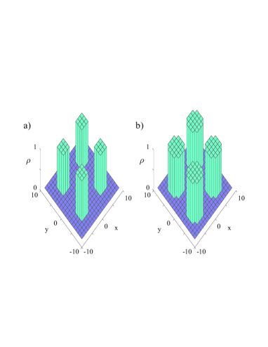
FIG. 3.: Superlattice potential in 2D with $V_{T}(x,y)=40J\;(\sin^{2}(\pi x/9a)+\sin^{2}(\pi y/9a))$ with the spacing between the lattice sites. The particle density $\rho(x,y)$ for four superlattice wells is shown. Parameters: a) $U=30J$ and $\mu=15J$, b) $U=50J$ and $\mu=27J$.

Using a Gutzwiller ansatz [75, 78, 79] for the wave function we have performed a mean field calculation to demonstrate how, by a proper choice of the potential $V_{T}({\bf x})$, one can fill certain blocks of the optical lattice with exactly one particle at temperature $T=0$. Figure 3 shows the result of this mean field calculation, a MI phase where the lattice sites are either filled with $0$ or $1$ particles. The number fluctuations are almost equal to zero and thus not shown in this plot. To achieve a MI phase at finite temperature $T\neq 0$ one has to fulfill the requirement $kT\ll U$ where the interaction strength $U$ gives the order of magnitude of the first excitation energy in a MI phase. One also has to ensure that particles do not move from a filled site with energy $\epsilon_{i}$ to an adjacent empty site with energy $\epsilon_{j}$ i.e. the temperature has to be much smaller than the energy difference between these two sites $kT\ll\epsilon_{j}-\epsilon_{i}$. In Sec. IV, we will need periodic fillings of optical lattices as shown in Fig. 3 to implement efficient multi-particle entanglement operations and for parallel quantum computing.

3 Moving the lattice potentials state selectively

We consider the example of alkali atoms with a nuclear spin equal to $3/2$ (⁸⁷Rb, ²³Na) trapped by standing waves in three dimensions and thus confined by a potential of the shape as given in Eq. (43). The internal states of interest are hyperfine levels corresponding to the ground state $S_{1/2}$ as shown in Fig. 5b. Along the $z$ axis, the standing waves are in the lin$\angle$lin configuration (two linearly polarized counter-propagating traveling waves with the electric fields $\vec{E}_{1}$ and $\vec{E}_{2}$ forming an angle $2\theta$ [80]) as shown in Fig. 4.

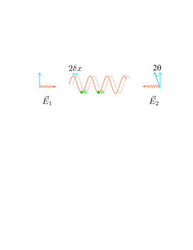
FIG. 4.: Laser configuration along the $z$-axis.

The total electric field is a superposition of right and left circularly polarized standing waves ($\sigma^{\pm}$) which can be shifted with respect to each other by changing $\theta$,

$$\vec{E}^{+}(z,t)=E_{0}e^{-i\nu t}\left[\vec{\epsilon}_{+}\sin(kz\!+\!\theta)+\vec{\epsilon}_{-}\sin(kz\!-\!\theta)\right],$$ (47)

where $\vec{\epsilon}_{\pm}$ denote unit right and left circular polarization vectors, $k=\nu/c$ is the laser wave vector and $E_{0}$ the amplitude. The lasers are tuned between the $P_{1/2}$ and $P_{3/2}$ levels so that the dynamical polarizabilities $\alpha_{\pm\mp}$ of the two fine structure $S_{1/2}$ states corresponding to $m_{s}=\pm 1/2$ due to the laser polarization $\sigma^{\mp}$ vanish ($\alpha_{+-}=\alpha_{-+}=0$), whereas the polarizabilities $\alpha_{\pm\pm}$ due to $\sigma^{\pm}$ are identical ($\alpha_{++}=\alpha_{-}\equiv\alpha$). This configuration is shown in Fig. 5a and can be achieved by tuning the lasers between the $P_{3/2}$ and $P_{1/2}$ fine state levels so that the ac-Stark shifts of these two levels cancel each other. The optical potentials for these two states are $V_{m_{s}=\pm 1/2}(z,\theta)=\alpha|E_{0}|^{2}\sin^{2}\left(kz\pm\theta\right)$.

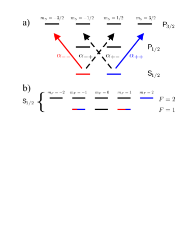
FIG. 5.: Level scheme of ⁸⁷Rb and ²³Na and laser configuration. (a) Fine structure energy levels and laser configuration. The detuning is chosen such that the polarizabilities $\alpha_{+-}$ and $\alpha_{-+}$ vanish. (b) Hyperfine level structure.

We choose for the states $|a\rangle$ and $|b\rangle$ the hyperfine structure states $|a\rangle\equiv|F=1,m_{f}=1\rangle$ and $|b\rangle\equiv|F=2,m_{f}=2\rangle$. Due to angular momentum conservation, these states are stable under collisions (for the dominant central electronic interaction [81, 82]). The potentials “seen” by the atoms in these internal states are

$$V^{a}(z,\theta) = \left[V_{m_{s}=1/2}(z,\theta)+3V_{m_{s}=-1/2}(z,\theta)\right]/4$$ (49)

$$V^{b}(z,\theta) = V_{m_{s}=1/2}(z,\theta).$$ (50)

If one stores atoms in these potentials and they are deep enough, there is no tunneling to neighboring wells and we can approximate them by harmonic potentials. By varying the angle $\theta$ from $\pi/2$ to $0$, the potentials $V^{b}$ and $V^{a}$ move in opposite directions until they completely overlap. Then, going back to $\theta=\pi/2$ the potentials return to their original positions. The shape of the potential $V^{a}$ changes as it moves. By choosing $\theta(t)=\pi\left(1-\left(1+\exp(-(\tau_{i}/\tau_{r})^{2})\right)/\left(1+\exp((t^{2}-\tau_{i}^{2})/\tau_{r}^{2})\right)\right)/2$ with $\tau_{r}=25/\omega$ and $\tau_{i}=25/\omega$, the frequencies and displacements of the harmonic potentials approximating (5) are exactly those plotted in Fig. 6a.

4 Gate fidelity

We use the minimum fidelity $F$ [83] to characterize the quality of the gate. $F$ is defined as

$$F=\min_{\varphi}\langle\tilde{\varphi}|{\rm tr}_{\rm ext}\left({\cal U}|\varphi\rangle\langle\varphi|\otimes\rho_{\rm ext}{\cal U}^{\dagger}\right)|\tilde{\varphi}\rangle,$$ (51)

where $|\varphi\rangle$ is an arbitrary internal state of both atoms, $|\tilde{\varphi}\rangle$ is the state resulting from $|\varphi\rangle$ using the mapping (13). The trace is taken over motional states, ${\cal U}$ is the evolution operator for the internal states coupled to the external motion (including the collision), and $\rho_{\rm ext}$ is the density operator corresponding to both atoms being at a temperature $T$ at time $t=-\tau$ [31]. In Fig. 6b the fidelity $F$ is plotted as a function of the temperature $T$ for the displacements and trap frequencies shown in Fig. 6a. This figure shows that one can achieve very high fidelities in realistic situations.

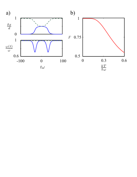
FIG. 6.: a) Upper plot: Displacements $\delta x^{a}(t)/d$ (solid line) and $1+\delta x^{b}(t)/d$ (dashed line). Lower plot: Trap frequencies $\omega^{a}(t)/\omega$ (solid line) and $\omega^{b}(t)/\omega$ (dashed line). b) Fidelity $F$ against temperature $kT/\hbar\omega$ for ⁸⁷Rb with $a_{s}=5.1{\rm nm}$. Here $\omega=2\pi\times 100{\rm kHz}$ and $d=390{\rm nm}$.

B Two-qubit gates in magnetic microtraps

We now consider the implementation of a switching potential by means of electromagnetic trapping forces. We first discuss the possibility of obtaining the desired state dependence by assuming some improvements on devices which are now experimentally available [84, 85, 86]. Then we compute the performance of a quantum gate for realistic trapping parameters.

1 Microscopic electromagnetic trapping potential

The interaction between the magnetic dipole moment of an atom in some hyperfine state $|F,m_{F}\rangle$ and an external static magnetic field $\vec{B}$ entails an energy $U_{\rm magn}\approx g_{F}\mu_{B}m_{F}|\vec{B}|$ depending on the atomic internal state via the quantum number $m_{F}$ (here $\mu_{B}$ is the Bohr magneton and $g_{F}$ is the Landé factor). On the other hand, the Stark shift induced on an atom by an electric field $\vec{E}$ gives a state-independent energy $U_{\rm el}\approx\frac{1}{2}\alpha|\vec{E}|^{2}$, where $\alpha$ is the atomic polarizability. The interplay between these two effects can be exploited in order to obtain a trapping potential whose shape depends on the atomic internal state. As an example, we consider an atomic mirror with an external magnetic field [84, 85, 86], providing confinement along two directions with trapping frequencies which can range from a few tens of kHz up to some MHz. Microscopic electrodes can be plugged on the mirror’s surface [87], thus allowing for the design of a potential with the characteristics described in Sect. II C.

2 Loading and moving atoms within the trap

Several schemes of loading atoms into the trap have been envisaged (see for example [84, 85, 86]). Most of them rely on an intermediate stage where atoms can be trapped and cooled without coming in contact with the magnetic mirror. This pre-loading trap can be either initially displaced from the surface, or close to it but based on a different trapping mechanism (for instance an evanescent wave mirror, where different internal states can be trapped by gravity [88] before the atoms can be put in the right states for magnetic trapping), to be replaced by the electromagnetic microtrap with a gradual switch-on of the electric and bias magnetic fields in the final stage of loading [87]. This could also allow for implementing a controlled filling of the trap sites, in a similar way to that already discussed in Sec. III A. A further feature to be implemented in view of performing more complex algorithms is the arrangement of several gate potentials in a periodic pattern, and the possibility of transporting atoms within this structure. An example would be given by two adjacent rows of potential minima, shiftable with respect to each other, where atoms could be loaded. A system like the one suggested in Sect. III B 1 could allow in principle to obtain such a configuration, since the magnetic field minima can be shifted parallel to the surface by rotating the bias magnetic field. In this way it should be possible to move some atoms, while holding others in place by means of additional local electric fields [84, 85, 86]. Provided that atoms can be addressed individually, which is needed even for performing a one-bit quantum gate, a procedure for implementing a simple quantum algorithm could be the following: perform a gate between two suitably chosen atoms, being close to each other but belonging to different rows, then mutually displace the rows and select another pair of atoms, including one of those coming out from the previous gate. Repeat until the algorithm has been operated, applying the required one-qubit rotations in between the above steps and possibly performing some of them in parallel.

3 Switching the trap potentials state selectively

We choose for the states $|a\rangle$ and $|b\rangle$ the same hyperfine structure states of ⁸⁷Rb considered in the previous Section, which are low-magnetic field seekers. If both particles are in state $|a\rangle$, there is no interaction-induced phase shift, as already discussed in Sec. II C 2. The results for both particles in state $|b\rangle$ are shown in Fig. 7.

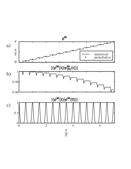
FIG. 7.: Dynamics during gate operation, with both atoms in state $\left|b\right\rangle$: a) interaction-induced phase shift - the circles refer to the perturbative calculation (33); b) projection of the evolved state on the corresponding state evolved without interaction; c) projection of the evolved state on the initial one. We choose $\omega\approx 23.4$ kHz and $\omega_{y}=\omega_{z}=150$ kHz, corresponding to ground-state widths $a_{x}\approx 50$ nm, $a_{y}=a_{z}\approx 28$ nm, with the initial wells having frequency $\omega_{0}=2\omega$ and displaced by $x_{0}=3\sqrt{2}a_{x}$. We take for the scattering length the known value for ⁸⁷Rb, i.e. $a_{s}^{bb}\approx a_{s}^{ab}=5.1$ nm. Time is in units of the oscillation period $T$.

The time dependence of $\phi^{bb}$ is step-like (Fig. 7a): the collisional phase is incremented at times $t_{k}\equiv(2k-1)T/4$, when the atoms meet at the center of the well, and remains constant at intermediate times, when they separate again. The influence of the interaction on the atomic motion can be seen from Fig. 7b, depicting the overlap between the evolved interacting two-atom state $|\psi^{bb}(t)\rangle$ and the corresponding state $|\psi^{bb}_{(0)}(t)\rangle$ computed without taking into account the interaction. The curve has local minima at times $t_{k}$, signalling that a collision is taking place, and shows a global decrease corresponding to a slight delay of the interacting motion with respect to the non-interacting one. As it can be seen from Fig. 7c, this effect is not dramatic: the oscillation period in the presence of interaction is increased just by $\delta T\approx 2\times 10^{-3}T$ (with the parameters used here), and the harmonic potential ensures that the system comes periodically back to its initial state. After $7$ oscillations we get a phase shift due to the interaction of $\pi$, whereas the perturbative formula (33) gives $7\phi^{bb}_{T}\approx 0.98\pi$. Therefore we choose $\tau=7(T+\delta T)\approx 0.15$ms: the overlap between the initial and the evolved wave function at that time is $|\langle\psi^{bb}(\tau)|\psi^{bb}(0)\rangle|^{2}\approx 0.996$. The behavior turns out to be quite different [89] when the atoms are in different internal states: the phase shift increases more rapidly, but after a few oscillations the system does no longer come back to the initial state. This has a simple explanation. The two atoms collide as soon as the one being in state $\left|b\right\rangle$, moving within the potential $m\omega^{2}x^{2}/2$, reaches its turning point, where the other atom is trapped. The interaction time is therefore longer than if both atoms were in state $\left|b\right\rangle$. Indeed, in that case they meet at the trap center, with their maximal velocity. This explains why the system picks up a bigger phase shift per oscillation period in the present case. On the other hand, the collision excites the motion of the atom in state $\left|a\right\rangle$ within its own well, and therefore the initial state is no longer recovered. This problem can be avoided if the potential minimum for state $\left|a\right\rangle$ is displaced along the transverse direction from the one for state $\left|b\right\rangle$ by means of an additional electrostatic field [84, 85, 86], so that the atoms interact if and only if they are both in state $\left|b\right\rangle$. This problem would not exist in an adiabatic scheme for the gate operation, when the shape of the potential is changed slowly with respect to the atomic motion. This will be the subject of future investigation.

4 Gate fidelity

The calculation of the fidelity in this case has to take into account the symmetrization of the wave function under particle interchange, expressed by an operator $S$ to be explicitly inserted into Eq. (51):

$$F=\min_{\varphi}\left\{{\rm tr}_{\rm ext}\left[\langle\tilde{\varphi}|{\cal U}S\left(|\varphi\rangle\langle\varphi|\otimes\rho_{\rm ext}\right)S^{\dagger}{\cal U}^{\dagger}|\tilde{\varphi}\rangle\right]\right\},$$ (52)

With the parameters quoted above, we obtain $F>0.98$. In order to reach such a fidelity, timing has to be quite precise, with a resolution of the order of $10^{-3}T$ corresponding to tens of ns in this case.

IV Parallel quantum computing

In this Section, we will discuss how quantum gates based on controlled collisions can be exploited for quantum computing. It is clear that, with the realization of a universal two-bit gate, any quantum computation can be performed, just as it is the case with other implementations. On the other hand, manipulations such as moving and switching potentials offer a great deal of parallelism [43, 44] not available in other systems.

We will focus our attention on implementations in optical lattices. Some of the ideas could readily be translated into arrays of magnetic microtraps, if the distances between the individual potential wells could be made much shorter than present-day state-of-the-art of nanofabrication. In such a situation, adiabatic variants of the switching operations (see comment at the beginning of Sec. II C) can be used to create multi-particle entangled clusters of neighboring atoms, similar as with moving potentials. Details of this analysis will be presented somewhere else [89].

One may ask, what can be done in optical lattices that cannot be done in other implementations? The answer to this question depends on a number of experimental conditions such as the possibility of creating regular filling structures and, like in ion-traps, on the possibility of addressing single atoms individually. In the following, we will first (Sec. IV A) give an example of what can be done with controlled lattice movements in conventional set-ups i.e. with random filling of the lattice sites and without any control of the position of individual atoms. We will see that this already allows one to perform interesting spectroscopic studies of the degree of entanglement between the atoms thus created. Next (Sec. IV B), we will describe what can be done if one achieves a regular occupation of the lattice sites and can address the atoms individually. Under such circumstances, an efficient implementation of quantum error correction and of a quantum memory (concatenated Shor code) is possible. Furthermore, fault tolerant versions of certain quantum gates and of quantum error correction can be implemented straightforwardly, as will be sketched in (Sec. IV C). Finally, in Sec. IV D, we describe how auxiliary atomic levels can be used to realize highly selective entanglement operations, where individually selected atoms are swept across the lattice to create GHZ states [90] of a large number of particles. Together with IV B and IV C, this scheme has all the ingredients that are necessary for an efficient realization of fault-tolerant quantum computing.

A Multi-particle entanglement operations

The two-qubit gates described in Sec. III correspond abstractly to an atom interferometer as shown in Fig. 8. The interferometer has two inputs which are the two atoms trapped at neighboring potential wells. By shifting the potentials back and forth as described in Secs. II B, only one combination of paths of the two particles overlaps and leads to a phase shift, namely the paths corresponding to state $|a\rangle_{1}$ for the left particle and $|b\rangle_{2}$ for the right particle. To emphasize the role of the internal states as logical states, we shall henceforth use the notation $|0\rangle\equiv|a\rangle$ and $|1\rangle\equiv|b\rangle$ and neglect the kinetic phases $\phi^{a}$, $\phi^{b}$ as they appear in (13). Furthermore, we drop the atomic index as long as there is no danger of confusion.

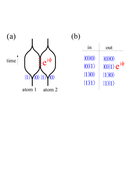
FIG. 8.: Atom-interferometric process realizing the quantum gate. (a) Two-particle interferometer; (b) Truth table.

The logical truth table corresponding to the interferometric process is shown in Fig. 8. [A similar identification of logical states can be made in magnetic traps as is pointed out in Sec. II C 4. The labelling of the paths for the left particle in the interferometer has to be interchanged in this case.] For $\phi=\phi^{01}=\pi$ this realizes a phase gate [1]. The phase gate and the set of all one-bit unitary transformations, which can be realized by Raman laser pulses on the internal states $|0\rangle$ and $|1\rangle$, define a universal set of quantum gates. [91, 92, 93, 94]

An important difference between optical lattices and other implementations is given by the global effect of the lattice manipulations. To illustrate this point, consider first a two dimensional lattice as in Fig. 9 with random occupation of the sites and a filling factor $\eta\ll 1$, where $\eta$ is defined as the average number of atoms per lattice site. Let us assume that the loading of the lattice can be accomplished in such a way that there are no multiply occupied lattice sites, i.e. that each lattice site is occupied by no more than a single atom.

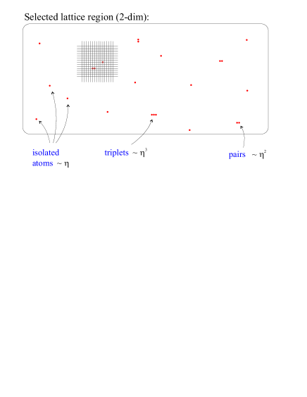
FIG. 9.: Random occupation of a two dimensional lattice with single atoms.

Then, in any region of the lattice, one will find isolated atoms, pairs of neighboring atoms, triplets, and so forth, with a relative frequency proportional to $\eta$, $\eta^{2}$, $\eta^{3},$ respectively. Consider now the following Ramsey experiment [95] where initially all atoms are prepared in the internal state $|0\rangle$ and in the motional ground state of their individual potential wells. In some selected region of the lattice, the following sequence of operations is applied: (1) a $\pi/2$ laser pulse brings all atoms into a superposition of the internal states $|0\rangle$ and $|1\rangle$; (2) the lattice is shifted across one lattice site and then, after a variable length of time, shifted back to its original position, (3) finally a second $\pi/2$ pulse is applied to the region. The effect of this sequence is illustrated in Fig. 10. For a group of $N=1,2,3,\dots$ neighboring atoms, the lattice shift corresponds to a N-particle interferometric process.

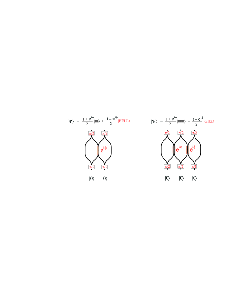
FIG. 10.: Entanglement of pairs (left) and triplets (right) of neighboring atoms by a single lattice shift.

Specifically, one obtains the following transformations. For isolated atoms:

$$|0\rangle\longrightarrow|0\rangle;$$ (53)

for pairs of neighboring atoms:

$$|00\rangle\longrightarrow\frac{1+e^{i\phi}}{2}|00\rangle+\frac{1-e^{i\phi}}{2}|\mbox{\sc bell}\rangle\,;$$ (54)

and for triplets of neighboring atoms:

$$|000\rangle\longrightarrow\frac{1+e^{i\phi}}{2}|000\rangle+\frac{1-e^{i\phi}}{2}|\mbox{\sc ghz}\rangle\,;$$ (55)

where we have used the notation

$$|\mbox{\sc bell}\rangle = \frac{1}{\sqrt{2}}\left\{|0\rangle|+\rangle-|1\rangle|-\rangle\right\}\,,$$ (56)

$$|\mbox{\sc ghz}\rangle = \frac{1}{\sqrt{2}}\left\{|0\rangle|+\rangle|1\rangle-|1\rangle|-\rangle|0\rangle\right\}\,,$$ (57)

and $|\pm\rangle=(|0\rangle\pm|1\rangle)/\sqrt{2}$. The expressions for groups of more particles become more complicated and shall be ignored in the present discussion. It is clear that for $\phi=\pi$ Bell- and GHZ states [96, 90] are created by a single lattice shift at various places within the region. This corresponds to an ensemble of 2-bit and 3-bit quantum gates, respectively, acting simultaneously at different lattice sites. To analyze the states (54) and (55) spectroscopically one could measure the state of the atoms in a final step of the above Ramsey sequence e.g. by a fluorescence measurement. It is clear that by such a measurement the entangled states will be destroyed. On the other hand, by repeating this sequence many times with different samples, one can measure the fluorescence signal as function of the phase $\phi$ (interaction time). Under ideal circumstances, all isolated atoms will remain in the dark state $|0\rangle$ while all fluorescence signals come from Bell ($\sim\eta^{2}$) or GHZ ($\sim\eta^{3}$) states [97]. To check that entangled states, rather than mixtures, are created in the process, the experiment is performed with different interaction times, e.g. times corresponding to $\phi=\pi$ and $\phi=2\pi$. For entangled states as in (54) and ( 55) all fluorescence signals will vanish at $\phi=2\pi$, while this will not be the case if the states created by the atomic collisions are mixtures of classical many-particle states. More generally, by measuring the visibility of the fluorescence signal one may study the fidelity of the entanglement created in the process, and its dependence on certain noise sources such as a finite temperature of the atoms. This way, the curve plotted in Fig. 6b) could be tested experimentally.

B Quantum error correction

To employ these entanglement operations for quantum computing, one has to have precise control over the number and the location of atoms that are involved in the collisional process. In addition to the ability of addressing single atoms, one therefore has to achieve a certain ordered occupation of the lattice sites. As described in Sec. III.A., Fig. 3, this can be by achieved by controlling the intensity of the trapping laser at sufficiently low temperatures. This way optical crystals with periodic patterns of atoms can be created as indicated in Figs. 11 and 15 [98]

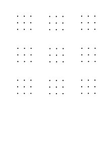
FIG. 11.: Ordered arrangement of atoms in an optical lattice (see also Fig. 3).

Under such circumstances the parallelism of the lattice manipulations can be exploited advantageously. On one side, similar logical operations can be performed simultaneously at different locations on the lattice. On the other side, as we have seen in Fig. 10, a single lattice shift can entangle whole groups of atoms. Two types of such entanglement operations are shown in Fig. 12. One involves only the logical states $|0\rangle$ and $|1\rangle,$ while the second uses a third atomic level as a “transport state” (see Sec. IV D), into which any atom must first be activated, before it can participate in an entanglement operation. In the following, we will first discuss applications of the shift operation as in Fig. 12(a). Later, in Sec. IV D we will consider a more flexible (“sweep”) operation shown in Fig. 12(b).

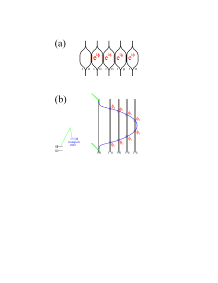
FIG. 12.: (a) “Shift operation”: The internal atomic states $|0\rangle$ and $|1\rangle$ couple to different lattice potentials that are moved against each other as explained in Sec. III A 3. This corresponds to a multi-particle interferometer where the same phase shift is acquired whenever two paths temporary overlap. By simple lattice manipulations, therefore, entire groups of atoms become entangled. (b) “Sweep operation”: For more selective entanglement operations, a third atomic level $|r\rangle$ is used [99]. In this scheme, only atoms in the level $|r\rangle$ are moved, whereas the states $|0\rangle$ and $|1\rangle$ are kept in the same potential. At the beginning of an entanglement operation, the atoms are first excited from one of the states $|0\rangle$ or $|1\rangle$ to the state $|r\rangle$ before the lattice is moved. This scheme is much more selective in the sense that those atoms which shall participate in a gate operation are first activated, before they couple to the moving lattice, and the collisional phases $\phi_{j}$ can be varied for each interaction individually.

An application of shift operations as described in Fig. 12(a) concerns the realization of a quantum memory, where a qubit $\alpha|0\rangle+\beta|1\rangle$ (with unknown coefficients $\alpha$ and $\beta$) is encoded in the quantum state of a larger block of atoms and stabilized against decoherence with the help of quantum error correction [47, 48, 49, 50, 51, 52, 53, 54]. A particular quantum code that is able to protect a qubit against general 1-bit errors (spin flip and phase flip) has been proposed by Shor [47]. It is a 9-bit code where the codewords

$$|0_{{\rm S}}\rangle = 2^{-3/2}(|000\rangle+|111\rangle)(|000\rangle+|111\rangle)(|000\rangle+|111\rangle)$$ (58)

$$|1_{{\rm S}}\rangle = 2^{-3/2}(|000\rangle-|111\rangle)(|000\rangle-|111\rangle)(|000\rangle-|111\rangle)$$ (59)

consist of products of certain GHZ states. Abstractly speaking, the encoding operation consists of a mapping (embedding) of the qubit’s 2-dimensional Hilbert space ${\cal H}$ into a $2^{9}$-dimensional Hilbert space of the form

$${\cal H}\ni\alpha|0\rangle+\beta|1\rangle\mapsto\alpha|0_{{\rm S}}\rangle+\beta|1_{{\rm S}}\rangle\in{\cal H}_{{\rm E}}\subset{\cal H}^{\otimes 9}.$$ (61)

To stabilize the encoded information against decoherence, the code must be measured and corrected on a time scale $\tau\ll 1/9\gamma$ where $\gamma$ is the rate of decoherence for a single qubit. This is possible since all errors that may occur on any one of the qubits of the codewords (LABEL:EQshorcode) map the code into a family of 2-dimensional subspaces of ${\cal H}^{\otimes 9}$ which are all orthogonal on ${\cal H}_{{\rm E}}$ [47].

The Shor code (LABEL:EQshorcode) can be implemented efficiently in a two dimensional lattice configuration [100] as in Fig. 11, by using the shift operation of Fig. 12(a).  To see this, imagine that the qubit/atom whose state is to be encoded is surrounded by neighboring atoms as in Fig. 13. The idea is of course to encode the central qubit in the whole block of $3\times 3$  qubits. Initially the central atom is in the unknown state $|\psi\rangle=\alpha|0\rangle+\beta|1\rangle$ while all neighboring atoms are in state $|0\rangle$. As is shown in Appendix B, the initial state is transformed into the Shor code by a simple sequence of horizontal and vertical lattice shifts combined with certain 1-bit rotations, as indicated in Fig. 13(a).  By this process, the information contained in $\psi$ is so to speak de-localized over the whole block of 9 atoms. To check whether an error has occurred on one of the qubits, the block is first decoded by  the inverse transformation [50], which involves the same sequence of lattice shifts as the encoding. Subsequently, one measures which of the neighboring atoms are in the state $|1\rangle$.

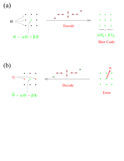
FIG. 13.: (a) Encoding of a qubit into a block of $3\times 3$ atoms; (b) Decoding and syndrome measurement.

In the language of quantum error correction, the surrounding atoms of the central qubit in Fig. 13(b) are the carriers of the error syndrome [50], meaning that their state gives information regarding what type of error occurred and, more importantly, which unitary 1-bit rotation has to be applied to the central qubit to restore it to the original state. In a fluorescence measurement, this information corresponds to a specific pattern of bright and dark atoms surrounding the central qubit. For example, in Fig. 13(b) a spin flip has occurred in the central qubit. This means that the state of the block is transformed into $\alpha\sigma_{x}^{{\rm ctr}}|0_{{\rm S}}\rangle+\beta\sigma_{x}^{{\rm ctr}}|1_{{\rm S}}\rangle$ where $\sigma_{x}^{{\rm ctr}}$ is the corresponding Pauli spin operator associated with the central atom. By the decoding operation of Fig. 13(b), this state is mapped into a product state of 9 qubits in which the neighboring atoms in the central row are both in the (bright) state $|1\rangle,$ while the other surrounding atoms are in the (dark) state $|0\rangle.$ The central atom is in a state equivalent to $|\psi\rangle$ up to a unitary transformation. Similar fluorescence patterns are obtained if a phase error occurs in the central atom or an arbitrary 1-bit error on any of the atoms in the block. A complete table of the error syndrome is given in the Appendix.

The essential point is that the measurement on the surrounding atoms does not reveal nor destroy the state of the central atoms (the coefficients $\alpha$ and $\beta$ remain unknown throughout the process). If the sequence of operations “decode-correct-encode” is repeated sufficiently often within the decoherence time $1/9\gamma$ of the block, the state $\psi$ may be protected over arbitrarily long times, in principle. Here one assumes, of course, that the decoding and encoding operations themselves are free of errors. In our situation this means that all phases acquired in the atomic collisions can be perfectly controlled. Since these operations will always bear some imperfection/imprecision, the probability that an error is introduced by an imperfect operation increases/accumulates with repeated applications of these operations. The general solution to this quantum-memory problem was given by Knill and Laflamme [57] and by others [58, 59, 60], and requires a concatenation of encoding operations as shown schematically in Fig. 14.

FIG. 14.: Concatenated quantum coding. At each coding level, a single qubit is encoded in a block of a larger number of qubits, here 5. (See e.g. [62]).

The number of required concatenation steps depends on how long the qubit is to be stored. It can be shown [57] that, given the precision of the operations is above a certain threshold, a qubit can be stored for an arbitrary long time, where the number of qubits required for encoding (i.e. the length of the code) grows polynomially with the length of the storage time. In the optical lattice configuration, a concatenation of the encoding can be implemented straightforwardly. Imagine that, in the central block in Fig. 11, the center atom is initially in state $|\psi\rangle=\alpha|0\rangle+\beta|1\rangle$ (similar as in Fig. 13) whereas all other atoms are in state $|0\rangle$. This means that both the surrounding atoms in the center block and the atoms of all the other blocks are initially in state $|0\rangle$. The first step of the encoding operation is identical as in Fig. 13 and results in the configuration where the center block is in a superposition of the Shor code words $|0_{{\rm S}}\rangle$ and $|1_{{\rm S}}\rangle,$ whereas the surrounding blocks remain in state $|0\rangle$. In the second step, the same operation is repeated on a larger scale, i.e. the lattice is shifted across a larger distance such as to make the blocks temporarily overlap while the 1-bit operations of the first step are now repeated on corresponding atoms of the outer blocks. As a result, the information $|\psi\rangle$ originally carried by the center atom is now delocalized over $9\times 9=81$ atoms! This scheme may be iterated as indicated in Fig. 15.

FIG. 15.: Concatenated quantum coding in an optical lattice. At each coding level, two-dimensional lattice displacements with an increasing periodicity are applied. The nested character of Fig. 14 is here reflected by a self-similar filling pattern of the lattice.

When in the second (and higher-order) encoding step the blocks are brought to overlap, one has to make sure that only phases between corresponding atoms of the different blocks are accumulated. The most elegant way to achieve this would be with the aid of a technique where the 0 and 1 states are displaced vertically before the atoms are moved. This could be implemented in a three-dimensional lattice configuration[101]. The shift operation is then really a “lift & shift” operation. The collisional interaction is then only switched on by varying the vertical displacement, after the blocks have been moved horizontally. If such a lifting technique can not be implemented, e.g. in a truly two-dimensional configuration, then during the horizontal motion there will be also collisions between non-corresponding atoms, for example the atoms in the right column of one of the blocks with atoms in the left column of a neighboring block. To avoid these unwanted phase shifts, it is possible to vary the velocity of the lattice movement in such a way that during unwanted collisions a phase of $e^{2\pi i}$ is acquired. This method is clearly more susceptible to decoherence. On the other hand, our numerical studies have shown [31], that by an appropriate choice of the displacement function $\theta(t)$ in Fig. 4, the phase of a single collision can, in principle, be controlled with a very high precision (with fidelity $\geq 0.9997$) and the probability for exciting phonons remains correspondingly small [102].

It does not seem impossible that $\theta(t)$ could be controlled precisely enough to meet the threshold of fault-tolerant computation [62], but we have not yet made detailed numerical investigations for this situation. In summary, the method of concatenated coding can be implemented in optical lattices by repeated sequences of lattice displacements on self-similar filling structures.

C Fault-tolerant computing

In a quantum computer, we do not only wish to store quantum information, but also to process it in a quantum algorithm. To prevent an accumulation of errors during the calculation due to imperfect gate operations, one needs to use fault-tolerant quantum gates that act on the encoded information. Furthermore, errors should be corrected fault tolerantly, that is, without decoding the information (and therefore exposing the qubit to decoherence). The general theory of fault-tolerant computation has been developed by several researchers [62]. In optical lattices, many of such fault-tolerant operations have a geometrically intuitive implementation. For example, if two qubits are encoded in blocks of 9 atoms each, as in Fig. 13, a controlled-NOT operation can be implemented by moving one block on top of the other so that each pair of corresponding atoms from the two blocks share a single potential well and acquire a phase shift $e^{i\pi}.$ [This is a straightforward generalization of the situation in Fig. 8].

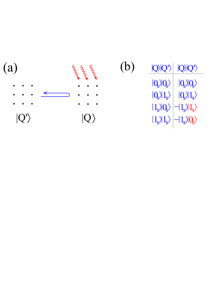
FIG. 16.: Implementation of a fault-tolerant CNOT gate.

When a $\pi/2$ pulse is applied on one of the blocks before and after the blocks are shifted, a fault-tolerant realization of the CNOT gate, with a truth table as in Fig. 16 is realized. The minus sign may be eliminated by applying a $3\pi/2$ pulse instead of the second $\pi/2$ pulse. Similarly, one can find a simple fault-tolerant realization of the NOT gate, while for example the Hadamard transform is more involved and requires a measurement with auxiliary qubits. Whether or not one can find similarly efficient implementations for a complete set of fault tolerant gates, is still under investigation.

To check whether an error has occurred during a gate operation, one has to measure whether the blocks are still in a superposition of the correct codewords. For the Shor code, this can be done in the following way [47], see Fig. 17: To detect a spin-flip, one has to measure the parity of the first two atoms in any row and compare it to the parity of the last two atoms of every row. To do this one would use an “Armada” of $3\times 2$ ancillas in the state $(|00\rangle+|11\rangle)(|00\rangle+|11\rangle)(|00\rangle+|11\rangle)$, which approaches the block from the left in Fig. 17 by moving the lattice horizontally.

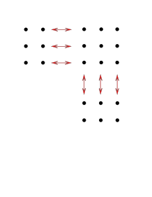
FIG. 17.: Implementation of fault-tolerant error correction.

To measure the parities, the Armada is moved on top of the first two columns of the data block so that the atoms interact pairwise with atoms of the data block and acquire a phase shift of $e^{i\pi}$. To satisfy the criteria for fault tolerance, we need to avoid collisions while the ancillas are moved on top of the code, and thus need a “lift & shift” implementation of the operation, as mentioned earlier. Suppose there was a spin-flip in one of the atoms of the first row. Then the state of the ancillary atoms after the interaction reads $(-|00\rangle+|11\rangle)(|00\rangle+|11\rangle)(|00\rangle+|11\rangle)$, and the error will be detected by measuring the parity of the ancillas in each row, after applying a Hadamard transform. In a second run, the Armada is reset in the initial state and then is moved on top of the last two rows of the block, and so on. To detect a phase-flip, a similar procedure is used with an Armada of $2\times 3$ atoms that approaches the block in Fig. 17 from below by moving the lattice vertically. Since these ancillas should measure any change of sign in any of the GHZ states that make up the codewords (LABEL:EQshorcode),  they have to be prepared in the state $|000000\rangle+|111111\rangle.$ A phase flip can then be detected as previously, where now a Hadamard transform has to be applied to the block first, before the “attack” starts from below. In the specific implementation using optical lattices, one could also think about other schemes using only a single row of ancilla atoms on each side of the data block in Fig. 17 as realized in Fig. 3b).

D Selectivity and “sweep operations”

The examples discussed so far make use of the parallelism of the lattice shift to implement certain multi-particle entanglement (or gate) operations efficiently. On the other hand, the shift operation as described in Fig. 12(a) is too rigid, when certain operations should apply to a selected group of atoms only. This problem can in principle be solved by using a third atomic level $|r\rangle$ as indicated in Fig. 12(b). In this scheme, the level $|r\rangle$ couples dominantly to a transport lattice [99], while the “logical states” $|0\rangle$ and $|1\rangle$ are kept in the same potential. At the beginning of an entanglement operation, the atoms are first excited from one of the states $|0\rangle$ or $|1\rangle$ to the state $|r\rangle,$ before the lattice is moved. This scheme is much more selective in the sense that those atoms which shall participate in a gate operation are first activated, before they can participate in the lattice movement. All operations that we have discussed can then be realized in the same manner, with the additional property that only those atoms, to which the operation $|1\rangle\rightarrow|{\rm r}\rangle$ is applied, will participate. With this additional feature, it is clear, that universal computations can be implemented.

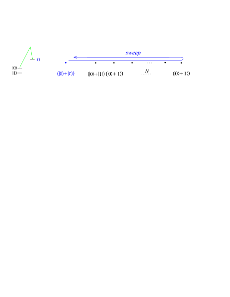
FIG. 18.: Realization of an $(N+1)$-dimensional GHZ state by a single sweep operation.

Another merit of this scheme is that one can realize more flexible entanglement operations. Consider, for example, a 1-dimensional situation as in Fig. 18 with a string of $N$ atoms initially prepared in the product state $(|0\rangle+|1\rangle)^{\otimes N}$ and a selected additional atom (left) in the state $(|0\rangle+|{\rm r\rangle)}$. By moving the transport lattice, the selected atom is swept across the $N$ lattice sites. During that motion, it interacts with each of the $N$ atoms thereby transforming the state of each atom into $e^{{i\phi^{0}}}|0\rangle+e^{i\phi^{1}}|1\rangle,$ with a differential phase $\phi=\phi^{1}-\phi^{0}.$ The resulting total state is of the form

$$|0\rangle(|0\rangle+|1\rangle)(|0\rangle+|1\rangle)\cdots(|0\rangle+|1\rangle)$$ (62)

$$+|{\rm r}\rangle e^{iN\phi^{0}}(|0\rangle+e^{i\phi}|1\rangle)(|0\rangle+e^{i\phi}|1\rangle)\cdots(|0\rangle+e^{i\phi}|1\rangle).$$ (63)

As long as the collisional phases are different ($\phi\neq 0$) for the two logical states, $\phi$ can by varied with the speed of this sweep operation. For $\phi=\pi$ one obtains a $N+1$ dimensional GHZ state (see Fig. 18 ) which can easily be brought to the standard form

$$|\psi\rangle=\frac{1}{\sqrt{2}}\left(|0\rangle|0\rangle|0\rangle\cdots|0\rangle+|1\rangle|1\rangle|1\rangle\cdots|1\rangle\right).$$ (64)

Note that for the creation of this state only a single sweep operation is required!

This scheme can be generalized in several directions. By varying the speed by which the lattice is moved during the sweep operation, the phases can be controlled individually for each atom of the string as indicated in Fig. 12, allowing for more complex entanglement operations. As a final example consider a configuration as in Fig. 19(b), with a “source register” consisting of a string of $m$ atoms in the state $|a\rangle=|a_{1}\;a_{2}\;a_{3}\;\cdots\;a_{m}\rangle$, $a_{j}\in\{0,1\}$ and a “target register” of $m$ further atoms in the state $(|0\rangle+|1\rangle)^{\otimes m}$, similar as in Fig. 18.

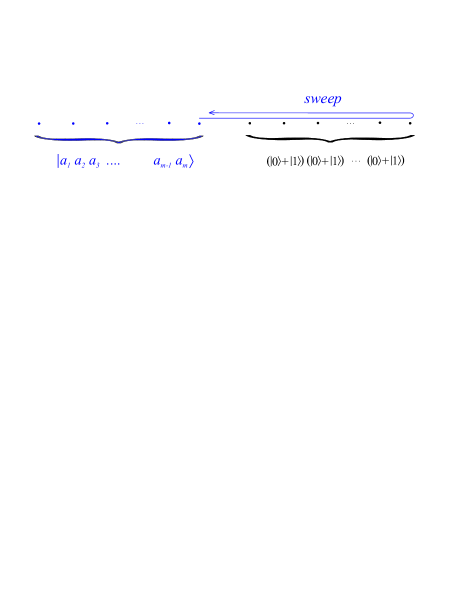
FIG. 19.: Implementation of the quantum Fourier transform by a sweep operation with variable speed.

The state vector $|a\rangle=|a_{1}\;a_{2}\;a_{3}\;\cdots\;a_{m}\rangle$ should be interpreted as a binary representation of the number $a=a_{1}2^{m-1}+a_{2}2^{m-2}+\dots+a_{m}2^{0}.$ Consider now the following operation where the source register is first activated to couple to the transport lattice, meaning that each of the atoms $1$ to $m$ that is in state $|1\rangle$  is excited to state $|r\rangle$. Next, the lattice is moved to the right so that atoms of the source and the target register interact; this motion continues with variable speed until the source register completely overlaps with the target register. It is helpful to mentally decompose this operation into discrete steps. In the first step, the transport lattice is shifted one lattice site to the right such that the $m$th atom of the source register interacts with the first atom of the target register. One can tune the interaction time such that a certain phase shift is acquired during this interaction, namely $\phi=2\pi/2^{m}$. In the next step, the transport lattice is moved one lattice site further to the right such that now the $m$ th atom of the source register interacts with the second atom of the target register, while at the same time the $m-1$ th atom of the source register interacts with the first atom of the target register. In this step, the interaction time is made double as long as in the first step, so that $\phi=2\pi/2^{m-1}$, and so on. After the lattice has been moved across $m$ sites in this vein, the total state of the source and the target register is given by

$$|a_{1}\;a_{2}\;a_{3}\; \cdots \;a_{m}\rangle\otimes(|0\rangle+e^{2\pi i0.a_{1}a_{2}\dots a_{m}}|1\rangle)$$ (67)

$$(|0\rangle+e^{2\pi i0.a_{2}\dots a_{m}}|1\rangle)$$

$$\quad\cdots\quad(|0\rangle+e^{2\pi i0.a_{m}}|1\rangle)\,.$$

Finally, the lattice is shifted back to the original position without changing the phases any more (modulo $2\pi$, see earlier remark, or the process can be made symmetric such that only half the phase values are accumulated during the motion to the right while the second halves of the phase values are accumulated when the lattice is brought back to its original position.) The overall effect of this sweep operation can be summarized in the form

$$|a\rangle|\quad\rangle\longrightarrow e^{i\Phi(a)}|a\rangle|{\cal F}(a)\rangle$$ (68)

wherein $|a\rangle$ and $|\quad\rangle$ denote the initial state of the source and the target register, and $|{\cal F}(a)\rangle$ is the discrete Fourier transform of the function $j\rightarrow a_{j}$. The additional phase factor $e^{i\Phi(a)}$ accounts for a possible phase shift arising from collisions among different atoms of the source, if no vertical displacement of the transport lattice is possible. It should be remarked that for a superposition of different input states the source and the target register become entangled, and therefore a direct application of this method in the Shor algorithm [103, 104] is not possible. Nevertheless, this final example demonstrates a remarkable flexibility of the entanglement operations that are possible in optical lattices and similar systems, offering new perspectives for efficient implementations of quantum algorithms.

V Final remarks

It is clear that, at the present time, most of the experimental requirements have yet to be realized, before one can implement quantum computing. There are, however, recent achievements in cooling and trapping of atoms in optical lattices and in magnetic microtraps which make it seem possible that some of these elements could be implemented in the laboratory in the near future. There are short-term and long-term perspectives. Essential for all quantum information experiments is a successful cooling of the atoms to the ground state of a three dimensional lattice. Numerical calculations [31] using realistic parameters give $kT<0.2\hbar\omega$ as a critical value. Under these circumstances, one could perform interesting Ramsey-type spectroscopic studies of the fidelity of multi-particle entanglement as discussed earlier. To do this, neither single-atom addressability is required nor are regular filling structures. When the latter requirements can be realized, on the other hand, coding experiments can be done and a quantum memory be implemented. Finally, if one can find three-level schemes with different scattering phases for the logical states, universal computations can be performed. The parallelism of the lattice could then be exploited for efficient implementations of fault-tolerant quantum computing.

We have discussed multi-particle entanglement schemes mainly in the context of optical lattice implementations. Some of these ideas could readily be adopted in implementations with magnetic microtraps if one uses adiabatic schemes. A basic requirement for this is the possibility of creating quantum dots that are spatially sufficiently close to each other. These ideas will be discussed somewhere else [89].

A One particle in a moving harmonic potential

1 Hamiltonian

The center of the potential with frequencies $\omega_{x}$, $\omega_{y}$ and $\omega_{z}$ is assumed to be given by $\bar{\bf x}(t)=(\bar{x}(t),0,0)$ and the Hamiltonian reads

$$H=H_{x}+H_{y}+H_{z},$$ (A1)

where $H_{z}=\hbar\omega_{z}(a_{z}^{\dagger}a_{z}+1/2)$, $H_{y}=\hbar\omega_{y}(a_{y}^{\dagger}a_{y}+1/2)$, and

$$H_{x}=\hbar\omega_{x}\left(a_{x}^{\dagger}a_{x}+\frac{1}{2}+(a^{\dagger}_{x}+a_{x})\frac{\bar{x}(t)}{\sqrt{2}}+\frac{\bar{x}(t)^{2}}{2}\right).$$ (A2)

The $a$’s are bosonic destruction operators and $\bar{x}(t)$ is given in harmonic oscillator units. We will concentrate on the $x$-direction leave out the subscript $x$ and normalize energies to $\hbar\omega$.

2 Exact solution

The Schrödinger equation for the Hamiltonian Eq. A2 can be solved exactly [105, 73]. To do so we define

$$H_{0}=a^{\dagger}a+\frac{1}{2},$$ (A3)

$$K(t,-\tau)=\frac{1}{\sqrt{2}}\int_{-\tau}^{t}ds\,\bar{x}(s)e^{i(s+\tau)}$$ (A4)

and

$$\beta(t,-\tau)=i\int_{-\tau}^{t}ds\,\left(K(s,-\tau)\{\partial_{s}K^{*}(s,-\tau)\}+\frac{i\bar{x}(s)^{2}}{2}\right).$$ (A5)

If initially at time $-\tau$ the system is in the state $|\Psi(-\tau)\rangle=|0\rangle$, where $|n\rangle$ is the $n$-th harmonic oscillator eigenstate we get

$$|\Psi(t)\rangle=e^{i\beta(t,-\tau)}\sum_{n}\frac{(iK(t,-\tau)e^{-i(t+\tau)})^{n}}{\sqrt{n!}}|n\rangle.$$ (A6)

The kinetic phase $\phi$ is thus given by the phase of the overlap of $|\Psi(t)\rangle$ with the instantaneous ground state $D({\bf\bar{x}}(t))|0\rangle$, where $D(\gamma)=\exp(\gamma a^{\dagger}-\gamma^{*}a)$ denotes the displacement operator

$$\phi=-{\rm arg}\left(\langle 0|D({\bf\bar{x}}(t))^{\dagger}|\Psi(t)\rangle\right).$$ (A7)

The interaction phase can be found by Eq. (7) with the known $|\Psi(t)\rangle$.

3 Corrections to the adiabatic approximation

We assume $\bar{x}(t)$ to be an analytic function of $t$ and that $\bar{x}(t)\gg\partial_{t}\bar{x}(t)\gg\partial_{t}^{2}\bar{x}(t)\gg\dots\gg\partial_{t}^{n}\bar{x}(t)$. By expanding in orders of the time derivatives we can write for $K(t^{\prime},-\tau)$

$$K(t^{\prime},-\tau) = \frac{1}{\sqrt{2}}\left(i^{N+1}\int_{-\tau}^{t^{\prime}}ds\{\partial^{N+1}_{s}\bar{x}(s)\}e^{i(s+\tau)}-\right.$$ (A9)

$$\left.\sum_{n=0}^{N}i^{n+1}\{\partial^{n}_{s}\bar{x}(s)\}e^{i(s+\tau)}|^{s=t^{\prime}}_{s=-\tau}\right),$$

where $N$ is a positive integer. Note that if we may neglect all terms of order greater than $\partial_{t}\bar{x}(t)$ and start in a coherent state $|\Psi(-\tau)\rangle=D(\bar{x}(-\tau)+i\partial_{t}\bar{x}(t)|_{t=-\tau})|0\rangle$ the state will always be a coherent state with $\langle x(t)\rangle=\bar{x}(t)$ and $\langle p(t)\rangle=\partial_{t}\bar{x}(t)$.

Now we assume for simplicity that $\bar{x}(\tau)=\bar{x}(-\tau)=0$, $(\partial_{t}\bar{x}(t))|_{t=-\tau}=(\partial_{t}\bar{x}(t))|_{t=\tau}=0$ and $(\partial^{n}_{t}\bar{x}(t))|_{t=-\tau}=(-1)^{n}(\partial^{n}_{t}\bar{x}(t))|_{t=\tau}$ for $n>1$. The system is assumed to be in the state $|\Psi(-\tau)\rangle=|0\rangle$, initially. We keep all the terms to fourth order in the derivatives (in the integrand) and find

$$K(t,-\tau) = \frac{1}{\sqrt{2}}\left(\left\{i(\partial^{2}_{t}-\partial^{4}_{t})\bar{x}(t)\right\}(e^{i(t+\tau)}-1)-\right.$$ (A11)

$$\left.\{\partial^{3}_{t}\bar{x}(t)\}(e^{i(t+\tau)}+1)\right),$$

and

$$\beta(t,-\tau) = \frac{1}{2}\int_{-\tau}^{t}ds\left(\{\partial_{s}\bar{x}(s)\}^{2}+\{\partial^{2}_{s}\bar{x}(s)\}^{2}\right)$$ (A13)

$$+\frac{1}{2}\{\partial^{2}_{s}\bar{x}(t)\}^{2}(1-e^{-i(t+\tau)}).$$

If we choose $(t+\tau)=2n\pi$ with integer $n$ the largest correction to the approximation to the kinetic phase discussed in Sec. II B 1 is of third order. Also the amplitude of the first excited state is of third order as can be seen from Eq. (A11).

B Quantum error correction and the implementation of Shor’s code

Consider a one-dimensional configuration with a string of $n$ atoms, where $x_{0},x_{1},x_{2},\dots,x_{n}\in\{0,1\}$ label the internal state of the atoms at position $0,1,2,\dots,n$ of the lattice. An elementary lattice-shift operation as given in Fig. 12(a) is then described as

$$LX: |x_{0},x_{1},x_{2},\dots,x_{n}\rangle\longmapsto$$ (B1)

$$e^{-i\sum_{j}(x_{j}+1\,{\rm mod}2)x_{j+1}\varphi_{j+1}}|x_{0},x_{1},x_{2},\dots,x_{n}\rangle$$ (B2)

where the phase $\varphi_{j+1}$ in the exponent depends on the interaction time and the interaction strength between two atoms at the lattice site $j+1$, and the addition is performed modulo 2. Note that two neighboring atoms at the sites $j$ and $j+1$ contribute to the exponent if and only if $x_{j}=0$ and $x_{j+1}=1$. The variables $x_{j}$ can only take on the values $0$ and $1$. In all examples we discuss here, $\varphi_{j}=\varphi=\rm constant$ and is the same for all lattice sites.

The operation (B2) defines a generalized phase gate that acts on a group of $n$ neighboring atoms via shifting the lattice across one lattice site. It can easily be seen that, for example when combined with $\pi/2$-pulses as in Fig. 10, LX produces the entangled states (54) and (55) for $n=2$ and $n=3$.

In two dimensional lattices, the logical variables $x_{kl}$ are labeled by two indices, where $k$ is the horizontal index and $l$ the vertical index. The phase gates corresponding to horizontal and vertical lattice shifts are then defined as

$$LX|\{x_{kl}\}\rangle = e^{-i\sum_{j}(x_{jl}+1\,{\rm mod}2)x_{j+1,l}\varphi_{j+1,l}}|\{x_{kl}\}\rangle$$ (B3)

$$LY|\{x_{kl}\}\rangle = e^{-i\sum_{j}(x_{kj}+1\,{\rm mod}2)x_{k,j+1}\varphi_{k,j+1}}|\{x_{kl}\}\rangle$$ (B4)

as an obvious generalization of (B2).

It is clear that the operations can be further generalized to lattice shifts across an arbitrary number of lattice sites and along arbitrary directions. There are interesting topological questions in this general situation. For the present discussion, however, the gates LX, LY as defined in (B4) are sufficient and we will set $\varphi_{k,l}=\pi$. Apart from these gates, we will only need single-particle operations, in particular the Pauli-operators $\sigma_{x,j},\sigma_{y,j},\sigma_{z,j}$ and the Hadamard transformation ($\pi/2$ pulse) $H_{j}=(\sigma_{z,j}+\sigma_{x,j})/\sqrt{2}$ applied to an atom with index $j$.

Consider now a configuration of $3\times 3$ atoms as in Fig. 13, where the central atom is in the unknown state $|\psi\rangle=\alpha|0\rangle+\beta|1\rangle$ while all surrounding atoms are initially in the state $|0\rangle$. Let us first look at the special case when $|\psi\rangle=|0\rangle$, that is, the central atom is in the state $|0\rangle$ as well. If we apply a $\pi/2$ pulse to each atom of the block and then the operation LX, we obtain a tensor product of three GHZ states where each row of the block is in the same state $(0+1)0(0-1)-(0-1)1(0+1)$. (For notational brevity, we suppress the bracket notation in the following and identify $0\equiv|0\rangle$ and $1\equiv|1\rangle$). This state can be transformed to the form $000-111$ by applying $H_{1}$ to the first atom and $H_{3}\sigma_{z,3}$ to the third atom of each row. The operation LX, supplemented by one-qubit rotations, produces thus one of the code words in (LABEL:EQshorcode).

To realize a quantum memory, an unknown state $\psi=\alpha 0+\beta 1$ of the central atom is to be encoded into an entangled 9-bit state as in (61). Let us write the initial (unencoded) state of the block in the form

$$|{\tt bare}\rangle=0_{1}0_{2}0_{3}\;0_{4}(\alpha 0_{5}+\beta 1_{5})0_{6}\;0_{7}0_{8}0_{9}$$ (B5)

where the first, second, and third triplet refers to the upper, center, and lower row of the block in Fig. 13. To encode $\psi$ into a corresponding superposition of both codewords, lattice movements in both horizontal and in vertical direction are required. In detail, the encoding operation is given by

$$ENC=H_{46}\circ LX\circ H_{456}\circ LY\circ\sigma_{x;369}H_{134679}\circ LX\circ H^{\rm s}$$ (B6)

whose essential part is a sequence of three lattice movements, horizontal - vertical - horizontal, with certain 1-bit unitary transformations in between. In the notation used here, $H^{\rm s}$ denotes a Hadamard transform applied to each of the 8 syndrome atoms, whereas $H_{ijk\dots}$ and $\sigma_{z;ijk\dots}$ are single-qubit rotations applied to the selected atoms $i$, $j$, $k$, $\dots$, only. Applied to the state (B5), $ENC$ produces

$$ENC\;|{\tt bare}\rangle = \alpha(000-111)(001-110)(000+111)$$ (B8)

$$\beta(000+111)(100+011)(000-111)$$

$$\equiv \alpha 0_{\rm L}+\beta 1_{\rm L}\,.$$ (B9)

The codewords $0_{\rm L}$ and $1_{\rm L}$ are equivalent to the Shor code (LABEL:EQshorcode), as we shall see presently.

The decoding operation is given by the inverse of (B6),

$$DEC=H^{\rm s}\circ LX\circ H_{134679}\sigma_{x;369}\circ LY\circ H_{456}\circ LX\circ H_{46}$$ (B10)

involving the same lattice movements, but the 1-bit operations carried out in reverse order. To see explicitly how one can correct an error occurring on one of the qubits $j=1,2,\dots 9$ , we apply the error operators $\sigma_{x,j}$, $\sigma_{y,j}$, or $\sigma_{z,j}$ to the encoded state $\alpha 0_{\rm L}+\beta 1_{\rm L}$. Then we apply the decoding operation $DEC$ and measure the state of the syndrome atoms. The code $0_{\rm L}$ and $1_{\rm L}$ is error correcting if every possible error is mapped into a syndrome state different from $0_{1}0_{2}0_{3}\;0_{4}0_{6}\;0_{7}0_{8}0_{9}$, and for each syndrome we can tell which unitary transformation has to be applied to the central qubit to restore it to its original state [it is not necessary that all errors are mapped to mutually orthogonal subspaces [47]]. The following table gives for each error the corresponding syndrome and the state of the central qubit:

error	syndrome	central qubit
none	000 00 000	$\alpha 0+\beta$ 1
$\sigma_{x,1}$	110 00 000	$\alpha 0-\beta$ 1
$\sigma_{x,2}$	101 00 000	$\alpha 0-\beta$ 1
$\sigma_{x,3}$	011 00 000	$\alpha 0-\beta$ 1
$\sigma_{x,4}$	010 10 010	$\alpha 0+\beta$ 1
$\sigma_{x,5}$	000 11 000	$\alpha 0-\beta$ 1
$\sigma_{x,6}$	010 01 010	$\alpha 0+\beta$ 1
$\sigma_{x,7}$	000 00 110	$\alpha 0-\beta$ 1
$\sigma_{x,8}$	000 00 101	$\alpha 0-\beta$ 1
$\sigma_{x,9}$	000 00 011	$\alpha 0-\beta$ 1
$\sigma_{y,1}$	100 00 000	$\alpha 0-\beta$ 1
$\sigma_{y,2}$	111 00 000	$\alpha 0-\beta$ 1
$\sigma_{y,3}$	001 00 000	$\alpha 0-\beta$ 1
$\sigma_{y,4}$	000 01 000	$\alpha 1-\beta$ 0
$\sigma_{y,5}$	010 00 010	$\alpha 1-\beta$ 0
$\sigma_{y,6}$	000 10 000	$\alpha 1-\beta$ 0
$\sigma_{y,7}$	000 00 100	$\alpha 0-\beta$ 1
$\sigma_{y,8}$	000 00 111	$\alpha 0-\beta$ 1
$\sigma_{y,9}$	000 00 001	$\alpha 0-\beta$ 1
$\sigma_{z,1}$	010 00 000	$\alpha 0+\beta$ 1
$\sigma_{z,2}$	010 00 000	$\alpha 0+\beta$ 1
$\sigma_{z,3}$	010 00 000	$\alpha 0+\beta$ 1
$\sigma_{z,4}$	010 11 010	$\alpha 1-\beta$ 0
$\sigma_{z,5}$	010 11 010	$\alpha 1+\beta$ 0
$\sigma_{z,6}$	010 11 010	$\alpha 1-\beta$ 0
$\sigma_{z,7}$	000 00 010	$\alpha 0+\beta$ 1
$\sigma_{z,8}$	000 00 010	$\alpha 0+\beta$ 1
$\sigma_{z,9}$	000 00 010	$\alpha 0+\beta$ 1

In Fig. 13, the syndrome atoms visually encircle the unknown qubit that is to be protected. If any of the 9 qubit suffers a spin flip, a phase flip, or both, the error can be detected by measuring the state of the syndrome atoms after the decoding operation has been applied to the group. This could be done by a fluorescence measurement where atoms in state 1 and 0 correspond to “bright” and “dark”, respectively. For example, according to above table, the pattern

0	0	0
1	$\psi^{\prime}$	1
0	0	0

tells us that a spin flip has occurred in the central atom, whereas

0	0	0
0	$\psi^{\prime}$	0
1	1	0

reveals a spin flip in the left atom of the lower row, and

0	1	0
1	$\psi^{\prime}$	1
0	1	0

corresponds to a phase flip in any of the atoms of the central row. In any case, the state $\psi^{\prime}$ of the central qubit after the detection of an error is related to the initial state $\psi$ via a (known) unitary operation $U$: $\psi^{\prime}=U\psi$, which can be obtained from the third column of the syndrome table given above.

The fact that the encoding operation involves only 3 lattice movements provides a specific example of a “parallelization of a quantum circuit” [43, 44]. We have not proven that 3 is really the minimum number of entanglement operations needed; there might be still faster sequences. The original Shor code can be recovered from this code by applying an additional vertical lattice shift, LY, and certain 1-bit rotations.

REFERENCES

- [1] Cirac, J. I., and Zoller, P., 1995, Phys. Rev. Lett. 74, 4091.
- [2] Monroe, C., Meekhof, D. M., King, B. E., Itano, W. M., and Wineland, D. J., 1995 Phys. Rev. Lett. 75, 4714.
- [3] Turchette, Q. A., Wood, C. S., King, B. E., Myatt, C. J., Leibfried, D., Itano, W. M., Monroe, C., and Wineland, D. J., 1998, Phys. Rev. Lett. 81 3631;
- [4] King, B.E., Myatt, C.J., Turchette, Q.A., Leibfried, D., Itano, W.M., Monroe, C., and Wineland, D.J., 1998, Phys. Rev. Lett. 81 1525;
- [5] Monroe, C., Leibfried, D., King, B.E., Meekhof, D.M., Itano, W.M., and Wineland, D.J., 1997, Phys. Rev. A 55, R2489.
- [6] Steane, A., 1997, Appl. Phys. B 64, 623.
- [7] Stevens, D., Brochard, J., and Steane, A., 1998, Phys. Rev. A 64, 623.
- [8] James, D.F.V., Gulley, M.S., Holzscheiter, M.H., Hughes, R.J., Kwiat, P.G., Lamoreaux, S.K., Peterson, C.G., Sandberg, V.D., Schauer, M.M., Simmons, C.M., Tupa, D., Wang, P.Z., and White, A.G., quant-ph/9807071.
- [9] Turchette, Q. A., Hood, C. J., Lange, W., Mabuchi, H., and Kimble, H. J., 1995, Phys. Rev. Lett. 75, 4710.
- [10] Maître, X., Hagley, E., Nogues, G., Wunderlich C., Goy, P., Brune, M., Raimond, J. M., and Haroche, S., 1997, Phys. Rev. Lett. 79, 769.
- [11] Hagley, E., Ma tre, X., Nogues, G., Wunderlich, C., Brune, M., Raimond, J. M., and S. Haroche, S., 1997, Phys. Rev. Lett. 79, 1.
- [12] Pellizzari, T., Gardiner, S.A., Cirac, J.I., and Zoller, P., 1995, Phys. Rev. Lett. 75, 3788.
- [13] Cirac, J. I., Zoller, P., Mabuchi, H., and Kimble, H. J., 1997, Phys. Rev. Lett. 78, 3221.
- [14] Van Enk, S. J., Cirac, J. I., and Zoller, P., 1998, Science 279, 205.
- [15] Law, C.K. and Kimble, H.J., 1997 J. Mod. Opt. 44, 2067.
- [16] Gheri, K.M. Saavedra, C., Törmä, P., Cirac, J.I., and Zoller, P., 1998, Phys. Rev. A 58, R2627.
- [17] Aspect, A., Grangier, P., and Roger, G., 1981, Phys. Rev. Lett. 47, 460.
- [18] Aspect, A., Grangier, P., and Roger, G., 1982, Phys. Rev. Lett. 49, 91.
- [19] Aspect, A., Dalibard, A., and Roger, G., 1982, Phys. Rev. Lett. 49, 1804.
- [20] Kwiat, P.G., Mattle, K., Weinfurter, H., Zeilinger, A., Sergienko, A.V., and Shih, Y.H., 1995, Phys. Rev. Lett. 75, 4337; Brendel, J., Gisin, N., Tittel, W., and Zbinden, H., quant-ph/9809034; Kwiat, P.G., Waks, E., White, A.G., Appelbaum, I., and Eberhard, P.H., quant-ph/9810003; Cabrillo, C. Cirac, J.I. Garcia-Fernandez, P., and Zoller, P., 1999, Phys. Rev. A 59, 1025.
- [21] Bouwmeester, D., Pan, J. I., Mattle, K., Eibl, M., Weinfurter, H., and Zeilinger, A., 1997, Nature 390, 575.
- [22] Boschi, D., Branca, S., De Martini, F., Hardy, L., and Popescu, S., 1998, Phys. Rev. Lett. 80, 1121.
- [23] Furusawa, A., Sorensen, J. L., Braunstein, S. L., Fuchs, C. A., Kimble, H. J., and Polzik, E. S., 1998, Science 282, 706.
- [24] Pan, J. W., Bouwmeester, D., Weinfurter, H., and Zeilinger, A., 1998, Phys. Rev. Lett. 80, 3891.
- [25] Boumeester, D., Pan, J.-W., Daniell, M., Weinfurter, H., and Zeilinger, A., 1999, Phys. Rev. Lett. 82, 1345.
- [26] Cory, D. G., Fahmy, A. F., and Havel, T. F., 1997, Proc. Natl. Acad. Sci. USA 94, 1634.
- [27] Gershenfeld, N. A., and Chuang, I. L., 1997, Science 275, 350.
- [28] Cory, D. G., Mass, W., Price, M., Knill, E., Laflamme, R., Zurek, W. H., Havel, T. F., and Somaroo, S. S., 1998, Phys. Rev. Lett. 81, 2152.
- [29] Jones, J. A., Mosca, M., and Hansen, R. H., 1998, Nature, 393, 344.
- [30] Braunstein, S.L., Caves, C.M., Jozsa, R., Linden, N., Popescu, S., and Schack R., quant-ph/9811018.
- [31] Jaksch, D., Briegel, H.-J., Cirac, J. I., Gardiner, C. W., and Zoller, P., 1999, Phys. Rev. Lett. 82, 1975.
- [32] Laser manipulation of Atoms and Ions,1992, edited by E. Arimondo, W. D. Phillips, and F. Strumia, (North Holland, Amsterdam); see also Special issue on Laser cooling and trapping of atoms, JOSA B 6 No. 11 (1989); ibid. 2 No. 11 (1985).
- [33] Chu, S., 1998, Rev. Mod. Phys. 70, 686.
- [34] Cohen-Tannoudji, C., 1998, Rev. Mod. Phys. 70, 707.
- [35] Phillips, W. D., 1998, Rev. Mod. Phys. 70, 721.
- [36] Anderson, M. H., Ensher, J. R., Matthews, M. R., Wieman, C. E., and Cornell, E. A., 1995, Science, 269, 198.
- [37] Bradley, C. C., Sackett, C. A., Tollett, J. J., and Hulet, R. G., 1995, Phys. Rev. Lett. 75, 1687.
- [38] Davies, K. B., Mewes, M.-O., Andrews, M. R., van Druten, N. J., Durfee, D. S., Kurn, D. M. and Ketterle, W., 1995, Phys. Rev. Lett. 75, 3969.
- [39] Hall, D. S., Matthews, M. R., Wieman, C. E., and Cornell, E. A., 1998, Phys. Rev. Lett. 81, 1543; ibid. 81, 4532.
- [40] Hall, D. S., Matthews, M. R., Ensher, J. R., Wieman, C. E., and Cornell, E. A., 1998, Phys. Rev. Lett. 81, 1539; ibid. 81, 4531.
- [41] Stamper-Kurn, D. M., Andrews, M. R., Chikkatur, A. P., Inouye, S., Miesner, H.-J., Stenger, J., and Ketterle, W., 1998, Phys. Rev. Lett.80, 2027.
- [42] Brennen, G.K., Caves, C.M., Jessen, P.S., and Deutsch, I.H., 1999, Phys. Rev. Lett. 82, 1060.
- [43] Moore, C., and Nilsson, M., 1998, Los Alamos preprint server quant-ph/9804034.
- [44] Moore, C., and Nilsson, M., 1998, Los Alamos preprint server quant-ph/9808027.
- [45] Freedman, M. H.,and Meyer, D. A., Los Alamos preprint server quant-ph/9810055.
- [46] Kitaev, A. Yu., and Bravyi, S. B., Los Alamos preprint server quant-ph/9811052.
- [47] Shor, P. W., 1995, Phys. Rev. A 52, R2493.
- [48] Steane, A. M., 1996, Phys. Rev. Lett. 77, 793; ibid., 1996, Proc. Roy. Soc. Lond. A 452, 2551.
- [49] Calderbank, A. R., and Shor, P. W., 1996, Phys. Rev. A 54, 1098.
- [50] Laflamme, R., Miquel, C., Paz, J.-P., and Zurek, W. H., 1996 Phys. Rev. Lett. 77, 198.
- [51] Ekert, A., and Macchiavello, C., 1996, Phys. Rev. Lett. 77, 2585.
- [52] Bennett, C. H., DiVincenzo, D. P., Smolin, J. A., and Wootters, W. K., 1996, Phys. Rev. A 54, 3825.
- [53] Knill, E., and Laflamme, R., 1997, Phys. Rev. A 55, 900.
- [54] For a review on the subject of quantum error correction (and on quantum computing in general) see, for example, Steane, A.M., 1998, Rept. Prog. Phys. 61, 117-173.
- [55] Shor, P. W., 1996, in Proc. 37th Symposium on the Foundations of Computer Science, (IEEE Computer Society Press), p. 56; quant-ph/9605011.
- [56] Steane, A. M., 1997, Phys. Rev. Lett. 78, 2252.
- [57] Knill, E., and Laflamme, R., 1996, quant-ph/9608012.
- [58] Aharonov, D., and Ben-Or, M., 1996, quant-ph/9611025.
- [59] Kitaev, A. Yu. 1997, Russ. Math. Surv. 52, 1191; ibid., quant-ph/9707021.
- [60] Knill, E., Laflamme, R., and Zurek, W., 1997, Science 279, 342.
- [61] Gottesman, D., 1998, Phys. Rev. A 57, 127.
- [62] For a review on the subject of fault-tolerant computing and for further references see, for example, Preskill, J., 1997, quant-ph/9705031.
- [63] Hamann, S.E., Haycock, D.L., Klose, G., Pax, P.H., Deutsch, I.H., and Jessen, P.S., 1998, Physical Review Letters 80 4149.
- [64] Mennerat-Robilliard, C., Lucas, D., Guibal, S., Tabosa, J., Jurczak, C., Courtois, J.-Y., and Grynberg, G., 1999, Physical Review Letters 82 851.
- [65] DePue, M. T. , McCormick, C. , Winoto, S.L. , Oliver, S. and Weiss, D.W., 1999, Physical Review Letters 82 2262.
- [66] Friebel, S., D’Andrea, C., Walz, J., Weitz, M., and Hänsch, T.W., 1998, Phys. Rev. A 57, R20.
- [67] Hinds, E. A., Boshier, M. G., and Hughes, I. G., 1998, Phys. Rev. Lett. 80, 645.
- [68] Weinstein, J.D., and Libbrecht, K.G., 1995, Phys. Rev. A 52, 4004.
- [69] Vuletic, V., Hänsch, T. W., and Zimmermann, C., 1996, Europhys. Lett. 36, 349.
- [70] Vuletic, V., Fischer, T., Praeger, M., Hänsch, T. W., and Zimmermann, C., 1998, Phys. Rev. Lett. 80, 1634.
- [71] Denschlag, J., Umshaus, G., and Schmiedmayer, J., 1998, Phys. Rev. Lett. 81, 737; Schmiedmayer, J., 1995, Phys. Rev. A 52, R13.
- [72] The justification parallels the arguments presented in the context of the pseudo-potential approximation in BEC see, e.g., H. T. C. Stoof, M. Bijlsma, and M. Houbiers, J. Res. Natl. Inst. Stand. Technol. 101, 443 (1996).
- [73] see, e.g., Galindo, A., Pascual, P., Quantum Mechanics II (Springer Berlin 1991).
- [74] Kagan, Yu., Surkov, E.L., and Shlyapnikov, G.V., 1996, Phys. Rev. A 54, R1753.
- [75] Jaksch, D., Bruder, C., Cirac, J. I., Gardiner, C. W., and Zoller, P, 1998 Phys. Rev. Lett. 81, 3108.
- [76] Fisher, M.P.A., Weichman, P.B., Grinstein, G., and Fisher, D.S., 1989, Phys. Rev. B 40, 546.
- [77] Bruder, C., Fazio, R., and Schön, G., 1993, Phys. Rev. B 47, 342.
- [78] Krauth, W., Caffarel, M., and Bouchard, J.-P., 1992, Phys. Rev. B 45, 3137.
- [79] Sheshadri, K., Krishnamurthy, H.R., Pandit, R., and Ramakrishnan, T. V., 1993, Europhys. Lett. 22, 257.
- [80] Finkelstein, V., Berman, P.R., and Guo, J., 1992, Phys. Rev. A, 45, 1829.
- [81] Weiner, J., Bagnato, V.S., Zilio, S., and Julienne, P.S., 1999, Rev. Mod. Phys. 71, 1.
- [82] Tiesinga, E., Verhaar, B.J., and Stoof, H.T.C., 1993, Phys. Rev. A, 47, 4114.
- [83] Schumacher, B., 1996, Phys. Rev. A 54, 2614.
- [84] Roach, T.M., Abele, H., Boshier, M.G., Grossman, H.L., Zetie, K.P., and Hinds, E.A., 1995, Phys. Rev. Lett. 75, 629.
- [85] Hinds, E.A., Boshier, M.G., and Hughes, I.G., 1998. Phys. Rev. Lett. 80, 645;
- [86] Hinds, E.A., 1999, to appear in Proc. R. Soc. London.
- [87] Schmiedmayer, J., 1998, Eur. Phys. J. D 4, 57.
- [88] Ovchinnikov, Yu.B., Manek, I., and Grimm, R., 1997, Phys. Rev. Lett. 79, 2225.
- [89] Calarco, T. et al., unpublished.
- [90] Greenberger, D. M., Horne, M., and Zeilinger, A., 1989, in Bell’s Theorem, Quantum Theory, and Conceptions of the Universe, M. Kafatos, editor, Kluwer, Dordrecht, The Netherlands, p. 69.
- [91] Barenco, A., Bennett, C.H., Cleve, R., DiVincenzo, D.P., Margolus, N., Shor, P., Sleator, T., Smolin, J.A., and Weinfurter, H., 1995, Phys. Rev. A 52, 3457; and references cited therein.
- [92] Deutsch, D., Barenco, A., and Ekert, A., 1995, quant-ph/9505018.
- [93] Bennett, C. H., 1995, Phys. Today 48, 24.
- [94] DiVincenzo, D. P., 1995, Phys. Rev. A 51, 1015.
- [95] N. F. Ramsey, Rev. Mod. Phys. 62, 541 (1990).
- [96] Bell, J.S., 1964, Physics 1, 195.
- [97] For small filling factors, the signals coming from different groups of atoms could even be spatially resolved.
- [98] Other proposals for selectively filling optical lattice sites exist (Martin Weitz, private communication), using infrared superlattices to load the (logical) lattice with a certain, well defined spacing between the atoms.
- [99] In 87Rb and 23Na one could use , and .
- [100] Freedman and Meyer [45] have independently identified Shor’s code as a two-dimensional topological quantum code (see also Kitaevs work [46, 59]). The connection between their results and our lattice implementation remains to be clarified.
- [101] Here we assume that one is able to selectively load a two-dimensional “sheet” in a three-dimensional lattice.
- [102] It remains the practical question, how well the polarization can be controlled in the experiment.
- [103] Shor, P. W., 1995, quant-ph/9508027; ibid., 1997, SIAM J. Computing 26, 1484.
- [104] Ekert, A., and Josza, R., 1996, Rev. Mod. Phys. 68, 733.
- [105] Gardiner, C.W., Quantum Noise (Springer Berlin 1991)