SONOLUMINESCENCE AND THE QED VACUUM 

In this talk I shall describe an extension of the quantum-vacuum approach to sonoluminescence proposed several years ago by J. Schwinger. We shall first consider a model calculation based on Bogolubov coefficients relating the QED vacuum in the presence of an expanded bubble to that in the presence of a collapsed bubble. In this way we shall derive an estimate for the spectrum and total energy emitted. This latter will be shown to be proportional to the volume of space over which the refractive index changes, as Schwinger predicted. After this preliminary check we shall deal with the physical constraints that any viable dynamical model for SL has to satisfy in order to fit the experimental data. We shall emphasize the importance of the timescale of the change in refractive index. This discussion will led us to propose a somewhat different version of dynamical Casimir effect in which the change in volume of the bubble is no longer the only source for the change in the refractive index.

1 Introduction

Sonoluminescence (SL) is the phenomenon of light emission by a sound-driven gas bubble in fluid $\!{}^{{\bf?}}$. The intensity of a standing sound wave can be increased until the pulsations of a bubble of gas trapped at a velocity node have sufficient amplitude to emit picosecond flashes of light. The basic mechanism of light production is still controversial. We shall start by presenting a brief summary of the main experimental data (as currently understood) and their sensitivities to external and internal conditions. The most common situation is that of an air bubble in water. SL experiments usually deal with bubbles of ambient radius $R_{\mathrm{a}mbient}\approx 4.5\;\mu{\rm m}$. The bubble is driven by a sound wave of frequency of $20-30$ kHz. During the expansion phase, the bubble radius reaches a maximum of order $R_{\mathrm{m}ax}\approx 45\;\mu{\rm m}$, followed by a rapid collapse down to a minimum radius of order $R_{\mathrm{m}ax}\approx 0.5\;\mu{\rm m}$. The photons emitted by such a pulsating bubble have typical wavelengths of the order of visible light. The minimum observed wavelengths range between $200\;{\rm nm}$ and $100\;{\rm nm}$. This light appears distributed with a power-law spectrum (with exponent depending on the noble gas admixture entrained in the bubble) with a cutoff in the extreme ultraviolet. If one fits the data to a Planck black-body spectrum the corresponding temperature is several tens of thousands of Kelvin (typically $70,000\;{\rm K}$, though estimates varying from $40,000\;{\rm K}$ to $100,000\;{\rm K}$ are common). There is considerable doubt as to whether or not this temperature parameter corresponds to any real physical temperature. There are about one million photons emitted per flash, and the average total power released is $30\;\hbox{ mW}\leq W\leq 100\;\hbox{ mW}$. The photons appear to be created in a very tiny spatio-temporal region: of order $10^{-1}\mu{\rm m}$ and on timescales $\tau\leq 50\;\hbox{\rm ps}$ (there have been claims that flash duration is less than $100\;{\rm fs}$, though more recent claims place flash duration in the range $50-250$ ps $\!{}^{{\bf?},{\bf?}}$). A truly successful theory of SL must also explain a whole series of characteristic sensitivities to different external and internal conditions. Among these dependencies the main one is surely the mysterious catalytic role of noble gas admixtures. Other external conditions that influence SL are magnetic fields and the temperature of the water (see $\!{}^{{\bf?}}$).

These are only the most salient experimental dependencies of the SL phenomenon. In explaining such detailed and specific behaviour the Casimir approach (the QED vacuum approach) encounters the same problems as other approaches have. Nevertheless we shall argue that SL explanations using a Casimir-like framework are viable.

1.1 Quasi-static Casimir models: Schwinger’s approach

The idea of a “Casimir route” to SL is due to Schwinger who several years ago wrote a series of papers $\!{}^{{\bf?},{\bf?},{\bf?},{\bf?},{\bf?},{\bf?},{\bf?}}$ regarding the so-called dynamical Casimir effect. Considerable confusion has been caused by Schwinger’s choice of the phrase “dynamical Casimir effect” to describe his model. In fact, his original model is not dynamical and is at best quasi-static as the heart of the model lies in comparing two static Casimir energy calculations: that for an expanded bubble with that for a collapsed bubble. Schwinger estimated the energy emitted during this collapse as being approximately equal to the change in the static Casimir energy. The static Casimir energy of a dielectric bubble (of dielectric constant $\epsilon_{{\mathrm{i}nside}}$) in a dielectric background (of dielectric constant $\epsilon_{{\mathrm{o}utside}}$) is

$$E_{cavity}=+\frac{1}{6\pi}\hbar cR^{3}K^{4}\left({1\over\sqrt{\epsilon_{\mathrm{\mathrm{i}nside}}}}-{1\over\sqrt{\epsilon_{\mathrm{\mathrm{o}utside}}}}\right)+\cdots.$$ (1)

Here the dots stand for additional sub-dominant finite volume effects $\!{}^{{\bf?},{\bf?},{\bf?}}$. The quantity $K$ is a high-wavenumber cutoff that characterizes the wavenumber at which the real parts of the refractive indices drop to their vacuum values. Hence $K$ is a physical cutoff given by condensed matter physics, not a regularization parameter to be renormalized away. This cutoff can be interpreted as the typical length scale beyond which the notion of a continuous dielectric medium is no longer meaningful. The result (1) can also be rephrased in the clearer and more general form as $\!{}^{{\bf?},{\bf?},{\bf?}}$:

$$E_{cavity}=+2V\int\frac{d^{3}\vec{k}}{(2\pi)^{3}}\;\frac{1}{2}\hbar\left[\omega_{\mathrm{\mathrm{i}nside}}(k)-\omega_{\mathrm{\mathrm{o}utside}}(k)\right]+\cdots$$ (2)

where it is evident that the Casimir energy can be interpreted as a difference in zero point energies due to the different dispersion relations inside and outside the bubble. In the case of SL $\omega_{\mathrm{i}nside}(k)\approx ck$, $\omega_{\mathrm{o}utside}(k)=ck/n$ for $k<K$, and $\omega_{\mathrm{o}utside}(k)\approx ck$ for $k>K$. In Schwinger’s original model he took $n\approx n_{\mathrm{l}iquid}\approx 1.33$, $R\approx R_{\mathrm{m}ax}$, and $K\approx 2\pi/400\;{\rm nm^{-1}}$, leading to about three million emitted photons $\!{}^{{\bf?}}$.

The three main strengths of models based on zero point fluctuations are:
1) The vacuum production of photon pairs allows for the very short timescales that one requires to fit data. Typically one expects these timescales to be of the order of the time that the zero point modes of the EM field takes to be correlated on the bubble scale. (Roughly the light-crossing time for the bubble.) For a bubble of radius $0.5$ microns this time scale is about $1.6$ femtoseconds, which is certainly sufficiently rapid to be compatible with observed flash duration.
2) One does not need to achieve “real” temperatures of thousands of Kelvin inside the bubble. Quasi-thermal behaviour is generated in quantum vacuum models by the squeezed nature of the two photon states created, and the “temperature” parameter is a measure of the squeezing, not a measure of any real physical temperature .
3) There is no actual production of far ultraviolet photons (because the refractive index goes to unity in the far ultraviolet) so one does not expect the dissociation effects in water that other models imply. Models based on the quantum vacuum automatically provide a cutoff in the far ultraviolet from the behaviour of the refractive index. Moreover this cutoff appears to be sensitive to the water temperature in such a way to explain the former described experimental dependencies—this observation going back to Schwinger’s first papers on the subject $\!{}^{{\bf?}}$.

Thus one key issue in Schwinger’s model is simply that of calculating static Casimir energies for dielectric spheres. It must be stressed that there is still considerable disagreement on this calculation. Milton, and Milton and Ng $\!{}^{{\bf?}}$ strongly criticize Schwinger’s result. These points have been discussed extensively in $\!{}^{{\bf?},{\bf?},{\bf?}}$ where it is emphasized that one has to compare two different geometrical configurations, and different quantum states, of the same spacetime regions. In a situation like Schwinger’s model for SL one has to subtract from the zero point energy (ZPE) for a vacuum bubble in water the ZPE for water filling all space. It is clear that in this case the bulk term is physical and must be taken into account. In the situation pertinent to sonoluminescence, the total volume occupied by the gas is not at all conserved (the gas is truly compressed), and it is far too naive to simply view the ingoing water as flowing coherently from infinity (leaving voids filled with air or vacuum somewhere in the apparatus). Since the density of water is approximately but not exactly constant, the influx of water will instead generate an outgoing density wave which will be rapidly damped by the viscosity of the fluid. The few phonons generated in this way are surely negligible.

1.2 Eberlein’s dynamical model for SL

The quantum-vacuum approach to SL was extended in the work of Eberlein $\!{}^{{\bf?}}$. The basic mechanism in Eberlein’s approach is a dynamical Casimir effect: Photons are produced due to a change of the refractive index in the portion of space between the minimum and the maximal bubble radius (a related discussion for time-varying refractive index is due to Yablonovitch $\!{}^{{\bf?}}$). This physical framework is actually implemented via a boundary between two dielectric media which accelerates with respect to the rest frame of the quantum vacuum state. The adiabatic change in the zero-point modes of the fields reflects in a non-zero radiation flux.

In the Eberlein analysis the motion of the bubble boundary is taken into account by introducing a velocity-dependent perturbation to the usual EM Hamiltonian:

$$H_{\epsilon} \!= \!\frac{1}{2}\int{\rm d}^{3}{\bf r}\left({{\bf D}^{2}\over\epsilon}+{\bf B}^{2}\right)\;,\>\>\>\Delta H\!=\!\beta\int{\rm d}^{3}{\bf r}\frac{\epsilon-1}{\epsilon}\;({\bf D}\wedge{\bf B})\cdot{\bf\hat{r}}\;.$$ (3)

This is an approximate low-velocity result coming from a power series expansion in the speed of the bubble wall $\beta=\dot{R}/c$. (The bubble wall is known to collapse with supersonic velocity, values of Mach 4 are often quoted, but this is still completely non-relativistic with $\beta\approx 10^{-5}$.)

Eberlein’s final result for the energy radiated over one acoustic cycle is:

$${\cal W}=1.16\>\frac{(n^{2}-1)^{2}}{n^{2}}\,\frac{1}{480\pi}\left[{\hbar\over c^{3}}\right]\int_{0}^{T}{\rm d}\tau\;\frac{\partial^{5}R^{2}(\tau)}{\partial\tau^{5}}\,R(\tau)\beta(\tau)\;.$$ (4)

(Eberlein approximates $n_{\mathrm{\mathrm{i}nside}}\approx n_{\mathrm{a}ir}\approx 1$ and sets $n_{\mathrm{\mathrm{o}utside}}=n_{\mathrm{w}ater}\to n$. The $1.16$ is the result of an integral is estimated numerically.) In this mechanism the massive burst of photons is produced at and near the turn-around at the minimum radius of the bubble. There the velocity rapidly changes sign, from collapse to re-expansion. This means that the acceleration is peaked at this moment, and so are higher derivatives of the velocity.

The main points of strength of the Eberlein model are the same as previously listed for the Schwinger model. However, Eberlein’s model exhibits a significant weakness (which does not apply to the Schwinger model):
The calculation is based on an adiabatic approximation which does not seem consistent with results . In order to fit the experimental values the model requires, as an external input, the bubble radius time dependence. This is expressed as a function of a parameter $\gamma$ which describes the time scale of the collapse and re-expansion process. In order to fit the experimental values for $\cal W$ one has to fix $\gamma\approx 10\;{\rm fs}$. This is far too short a time to be compatible with the adiabatic approximation. Although one might claim that this number can ultimately be modified by the eventual inclusion of resonances it would seem reasonable to take this ten femtosecond figure as a first self-consistent approximation for the characteristic timescale of the driving system (the pulsating bubble). Unfortunately, the characteristic timescale of the collapsing bubble then comes out to be of the same order of the characteristic period of the emitted photons. This shows that attempts at bootstrapping the calculation into self-consistency instead bring it to a regime where the adiabatic approximation underlying the scheme cannot be trusted.

This discussion has lead us to discover a quite intricate situation. We have on the one hand simple estimates of the vacuum energy that can be involved in SL, estimates that are still the object of heated debate, and on the other hand we have a dynamical approach to the problem that seems to be partially self contradictory. In order to resolve the first issue and to understand the proper framework to deal with the second we shall now consider what we can best view as a “toy model”. In spite of its simplicity this toy model will allow us to capture some basic results that we hope will guide future research on the “Casimir route” to sonoluminescence.

2 Bogolubov approach on a single oscillation

Let us consider a single pulsation of the bubble. At this stage of development, we are not concerned with the dynamics of the bubble surface. In analogy with the subtraction procedure of the static calculations of Schwinger $\!{}^{{\bf?},{\bf?},{\bf?},{\bf?},{\bf?},{\bf?},{\bf?}}$ or of Carlson et al. $\!{}^{{\bf?},{\bf?},{\bf?}}$ we shall consider two different configurations of space. An “in” configuration with a bubble of dielectric constant $\epsilon_{\mathrm{\mathrm{i}nside}}$ (typically vacuum) in a medium of dielectric constant $\epsilon_{\mathrm{\mathrm{o}utside}}$, and an “out” one in which one has just the latter medium (dielectric constant $\epsilon_{\mathrm{\mathrm{o}utside}}$) filling all space. These two configurations will correspond to two different bases for the quantization of the field. (For the sake of simplicity we take, as Schwinger did, only the electric part of QED, reducing the problem to a type of scalar electrodynamics). The two bases will be related by Bogolubov coefficients in the usual way. Once we determine these coefficients we easily get the number of created particles per mode and from this the spectrum. We shall also make a consistency check by a direct confrontation between the change in static Casimir energy and the sum, $E=\sum_{k}\omega_{k}n_{k}$, of the energies of the emitted photons.

2.1 Bogolubov coefficients

We use the Schwinger framework. In spherical coordinates and with a time independent dielectric constant

$$\epsilon{\partial^{2}\over\partial t^{2}}E-\nabla^{2}E=0.$$ (5)

Solutions are of the form

$$E=e^{i\omega t}{G(r)\over\sqrt{r}}Y_{lm}(\Omega).$$ (6)

Then one finds

$$G^{{}^{\prime\prime}}+{1\over r}G^{{}^{\prime}}+\left(\lambda^{2}-{(l+1/2)^{2}\over r^{2}}\right)G=0.$$ (7)

where $\lambda^{2}=\epsilon\omega^{2}$. This is the standard Bessel equation, it admits as solutions Bessel functions of the first kind, $J_{\nu}(\lambda r)$, and Neumann functions, $N_{\nu}(\lambda r)$ (Bessel functions of the second kind), with $\nu=l+1/2$.

For the “in” QED vacuum we have to take into account that the dielectric constant changes at the bubble wall. In fact we have

$$\epsilon=\left\{\begin{array}[]{llll}\epsilon_{1}&=&\mbox{dielectric constant of air}&\mbox{if $r<R$},\\ \epsilon_{2}&=&\mbox{dielectric constant of water}&\mbox{if $r>R$.}\end{array}\right.$$ (8)

We now use the fact that the dielectric constant of air is approximately equal 1 and shall deal only with the constant of water ($n=\sqrt{\epsilon_{2}}\approx 1.3$) For the eigenmodes of the “in” state one has

$$G^{\mathrm{i}n}_{\nu}(n,\omega,r)=\left\{\begin{array}[]{ll}A_{\nu}J_{\nu}(\omega_{\mathrm{i}n}r)&\mbox{if $r<R$,}\\ B_{\nu}J_{\nu}(n\omega_{\mathrm{i}n}r)+C_{\nu}N_{\nu}(n\omega_{\mathrm{i}n}r)&\mbox{if $r>R$.}\end{array}\right.$$ (9)

The coefficients $A_{\nu}$, $B_{\nu}$ and $C_{\nu}$ are determined by the matching conditions

$$\begin{array}[]{lll}A_{\nu}J_{\nu}(\omega_{\mathrm{i}n}R)&=&B_{\nu}J_{\nu}(n\omega_{\mathrm{i}n}R)+C_{\nu}N_{\nu}(n\omega_{\mathrm{i}n}R),\\ A_{\lambda}J_{\nu}{{}^{\prime}}(\omega_{\mathrm{i}n}R)&=&B_{\nu}J_{\nu}{{}^{\prime}}(n\omega_{\mathrm{i}n}R)+C_{\nu}N_{\nu}{{}^{\prime}}(n\omega_{\mathrm{i}n}R).\end{array}$$ (10)

The eigenmodes for the “out” QED vacuum are easily obtained solving the same equation but for a space filled with an homogeneous dielectric .

$$G^{\mathrm{o}ut}_{\nu}(n,\omega_{\mathrm{o}ut},r)=J_{\nu}(n\omega_{\mathrm{o}ut}r).$$ (11)

The Bogolubov coefficients are defined as

$$\alpha_{ij} = ({E_{i}^{\mathrm{o}ut}},{E_{j}^{\mathrm{i}n}}),\>\>\>\beta_{ij}=({E_{i}^{\mathrm{o}ut}}^{*},{E_{j}^{\mathrm{i}n}})$$ (12)

where the naive scalar product is as usual 

$$(\phi_{1},\phi_{2})=+i\int_{\Sigma}\phi_{1}^{*}\stackrel{{\scriptstyle\leftrightarrow}}{{\partial}}_{0}\phi_{2}\>d^{3}x.$$ (13)

We are mainly interested in the coefficient $\beta$ since $|\beta|^{2}$ is linked to the total number of particles created. By a direct substitution it is easy to find

$$\beta = (\omega_{\mathrm{i}n}-\omega_{\mathrm{o}ut})e^{i(\omega_{\mathrm{o}ut}+\omega_{\mathrm{i}n})t}\delta_{ll^{\prime}}\delta_{m,-m^{\prime}}$$ (14)

$$\qquad\int_{0}^{\infty}G^{\mathrm{o}ut}_{l}(n,\omega_{\mathrm{o}ut},r)\;G^{\mathrm{i}n}_{l^{\prime}}(n,\omega_{\mathrm{i}n},r)\>rdr.$$

After some work, the squared $\beta$ coefficients summed over $l$ and $m$ can be shown to be $\!{}^{{\bf?},{\bf?}}$

$$\left|\beta(\omega_{\mathrm{i}n},\omega_{\mathrm{o}ut})\right|^{2} = \left(\frac{n^{2}-1}{n^{2}}\frac{\omega_{\mathrm{i}n}^{2}R}{\omega_{\mathrm{o}ut}+\omega_{\mathrm{i}n}}\right)^{2}\sum_{\nu}(2\nu)\left|A_{\nu}\right|^{2}$$ (15)

$$\times\left[\frac{W[J_{\nu}(n\omega_{\mathrm{o}ut}r),J_{\nu}(\omega_{\mathrm{i}n}r)]_{R}}{(n\omega_{\mathrm{o}ut})^{2}-\omega_{\mathrm{i}n}^{2}}\right]^{2}.$$

The number spectrum and total energy content of the emitted photons are

$${dN(\omega_{\mathrm{o}ut})\over d\omega_{\mathrm{o}ut}} = \left(\int|\beta(\omega_{\mathrm{i}n},\omega_{\mathrm{o}ut})|^{2}d\omega_{\mathrm{i}n}\right),$$ (16)

$$E = \hbar\int{dN(\omega_{\mathrm{o}ut})\over d\omega_{\mathrm{o}ut}}\;\omega_{\mathrm{o}ut}\;d\omega_{\mathrm{o}ut}.$$ (17)

These expressions are too complex to allow an analytical resolution of the problem (except for the $R\to\infty$ limit).

2.2 Large-volume analytic limit

In this limit the total energy emitted should be approximately equal to the leading contribution in $R$ of the Casimir energy in the “in” state (a volume term if Schwinger was qualitatively correct, a surface or curvature one otherwise). Technically, if $R$ is very large (but finite in order to avoid infra-red divergences) then the “in” and the “out” modes can both be approximated by ordinary Bessel functions: $G^{\mathrm{i}n}(n,\omega,r)\approx J_{\nu}(\omega_{\mathrm{i}n}r)$, $G^{\mathrm{o}ut}(n,\omega,r)\approx J_{\nu}(n\omega_{\mathrm{o}ut}r)$. The Bogolubov coefficients simplify

$$\beta_{ij}=({E^{\mathrm{o}ut}_{i}}^{*},E^{\mathrm{i}n}_{j})\approx\left(1-\frac{1}{n}\right)e^{i\omega_{\mathrm{i}n}(1/n+1)t}\delta_{ll^{\prime}}\delta_{m,-m^{\prime}}\delta(\omega_{\mathrm{i}n}-n\omega_{\mathrm{o}ut}).$$ (18)

This implies

$$|\beta(\omega_{\mathrm{i}n},\omega_{\mathrm{o}ut})|^{2} \approx \left(1-\frac{1}{n}\right)^{2}\sum_{l}(2l+1){R\over 2\pi c}\delta(\omega_{\mathrm{i}n}-n\omega_{\mathrm{o}ut}),$$ (19)

where we have invoked the standard scattering theory result that $(\delta^{3}(k))^{2}=V\delta^{3}(k)/(2\pi)^{3}$, specialized to the fact that we have a 1-dimensional delta function. The summation over angular momenta can be estimated as $\!{}^{{\bf?}}$

$$\sum_{l=0}^{l_{\mathrm{m}ax}}(2l+1)\approx l_{\mathrm{m}ax}^{2}(\omega_{\mathrm{o}ut}) \approx \left(R\,n\,\frac{\omega_{\mathrm{o}ut}}{c}\right)^{2}.$$ (20)

This finally gives

$$|\beta(\omega_{\mathrm{i}n},\omega_{\mathrm{o}ut})|^{2} \approx \left(n-1\right)^{2}{R^{3}\over 2\pi c^{3}}\omega_{\mathrm{o}ut}^{2}\;\delta(\omega_{\mathrm{i}n}-n\;\omega_{\mathrm{o}ut}).$$ (21)

We can now compute the spectrum and the total energy of the emitted photons

$${dN(\omega_{\mathrm{o}ut})\over d\omega_{\mathrm{o}ut}}\approx n^{2}\;\left({n-1}\over{n}\right)^{2}\;\frac{R^{3}\omega_{\mathrm{o}ut}^{2}}{2\pi c^{3}}\;\Theta(K-n\,\omega_{\mathrm{o}ut}/c),$$ (22)

and

$$E\approx\frac{1}{8\pi\,n^{2}}\;\left({n-1}\over{n}\right)^{2}\hbar cK\;(RK)^{3}.$$ (23)

Hence, inserting our results (21) into Eqs. (16) for $dN(\omega)/d\omega$ and $E$, we deduce a spectrum that is proportional to phase space (and hence is a power law), up to the cutoff frequency where $n\to 1$. We interpret this as definitive proof that indeed Schwinger was qualitatively right: The main contribution to the Casimir energy of a (large) dielectric bubble is a bulk effect. The total energy radiated in photons balances the change in the Casimir energy up to factors of order one which the present analysis is too crude to detect. (For infinite volume the whole calculation can be re-phrased in terms of plane waves to accurately fix the last few prefactors.)

It is important to stress that Eq. (1) and Eq. (23) are not identical (even if in the large $R$ limit the leading term of Casimir energy of the “in” state and the total photon energy coincide). One can easy see that the volume term we just found [Eq. (23)] is of second order in $(n-1)$ and not of first order like Eq. (1). This is ultimately due to the fact that the interaction term responsible for converting the initial energy in photons is a pairwise squeezing operator $\!{}^{{\bf?}}$. Equation (23) demonstrates that any argument that attempts to deny the relevance of volume terms to sonoluminescence due to their dependence on $(n-1)$ has to be carefully reassessed. In fact what you measure when the refractive index in a given volume of space changes is not directly the static Casimir energy of the “in” state, but rather the fraction of this static Casimir energy that is converted into photons. We have just seen that once conversion efficiencies are taken into account, the volume dependence is conserved, but not the power in the difference of the refractive index .

2.3 Finite-volume numerical estimates:

For finite volume one can no longer rely on analytic results. Fortunately we know that for the total Casimir energy the next subdominant term is a surface area term that is suppressed by a factor of the cutoff wavelength divided by the bubble radius $\!{}^{{\bf?}}$. Canonical estimates are: $\lambda_{\mathrm{c}utoff}/R_{\mathrm{m}ax}\approx 0.3\;\mu{\rm m}/45\;\mu{\rm m}\approx 1/150$. This suggests that the effects of finite bubble size will not be too dramatic ($1\%$ in total energy?). Applying a mixture of semi-analytic and numerical techniques  to formula (15) we numerically derive the spectrum $dN/d\omega$ given in Fig. 1. For comparison we have also plotted the large volume analytic approximation (i.e., the leading bulk term by itself).

\begin{picture}(0.0,0.0)\centerline{\hbox{\psfig{height=227.62204pt,angle=270}}} \end{picture}

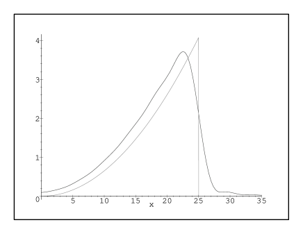
Figure 1: Spectrum obtained by numerical estimate for finite volume. We have made $R\approx R_{ambient}\approx 4.5\mu m$ and $\omega_{\mathrm{c}utoff}\approx 10^{15}Hz$. The sharply peaked curve is that appropriate to the (re-scaled) infinite volume limit (Schwinger limit).

2.4 Comment on the calculation

The lessons we have learned from this test calculation are:

(1) The model proves (in an indirect way) that the Casimir energy liberated via the bubble collapse includes (in the large $R$ limit) a term proportional to the volume (actually to the volume over which the refractive index changes). In the case of a truly dynamical model one expects that the energy of the photons so created will be provided by other sources of energy (e.g., the sound wave), nevertheless the presence of a volume contribution appears unavoidable.

(2) In spite of its simplicity (remember that the model is still semi-static), the present calculation is already able to fit some of the experimental requirements, like the shape of the spectrum and the number of emitted photons in the case of $R=R_{\mathrm{m}ax}$.

Of course the present model is still unable to fully fit other experimental features. For example it provides (like the original Schwinger model) maximal photon release at maximum expansion, and it is able to accommodate only a few arguments to explain the experimental dependencies. This means that a fully dynamical calculation is required in order to deal with these issues, and it is in order to understand what sort of model will ultimately be required that we shall now discuss in detail some basic features of sonoluminescence.

3 Hints towards a truly dynamical model

One of the key features of photon production by a space-dependent and time-dependent refractive index is that for a change occurring on a timescale $\tau$, the amount of photon production is exponentially suppressed by an amount $\exp(-\omega\tau)$. In an Appendix of $\!{}^{{\bf?}}$ we provided a specific toy model that exhibits this behaviour, and argued that the result is in fact generic.

The importance for SL is that the experimental spectrum is not  exponentially suppressed at least out to the far ultraviolet. Therefore any mechanism of Casimir-induced photon production based on an adiabatic approximation is destined to failure: Since the exponential suppression is not visible out to $\omega\approx 10^{15}\;\hbox{Hz}$, it follows that if  SL is to be attributed to photon production from a time-dependent refractive index (i.e., the dynamical Casimir effect), then the timescale for change in the refractive index must be of order of a femtosecond . Thus any Casimir–based model has to take into account that the change in the refractive index cannot be due just to the change in the bubble radius.

This means that one has to divorce the change in refractive index from direct coupling to the bubble wall motion, and instead ask for a rapid change in the refractive index of the entrained gases as they are compressed down to their van der Waals hard core. Yablonovitch $\!{}^{{\bf?}}$ has emphasized that there are a number of physical processes that can lead to significant changes in the refractive index on a sub-picosecond timescale. In particular, a sudden ionization of the gas compressed in the bubble would lead to an abrupt change, from $1$ to $\approx 0$, of the dielectric constant.

Now to get femtosecond changes in refractive index over a distance of about 100 nm (which is the typical length scale of the emission zone), the change in refractive index has to propagate at about $10^{8}$ metres/sec, about 1/3 lightspeed. To achieve this, one has to adjust basic aspects of the model: we feel that we must move away from the original Schwinger suggestion, in that it is no longer the collapse from $R_{\mathrm{m}ax}$ to $R_{\mathrm{m}in}$ that is important. Instead we postulate a rapid (femtosecond) change in refractive index of the gas bubble when it hits the van der Waals hard core $\!{}^{{\bf?}}$.

We stress that this conclusion, though it moves slightly away from the original Schwinger proposal, is still firmly within the realm of the dynamical Casimir effect approach to sonoluminescence. The fact is that the present work shows clearly that a viable Casimir “route” to SL cannot avoid a “fierce marriage” between QFT and features related to condensed matter physics.

It is thus crucial to look for possible unequivocal signatures of the dynamical Casimir effect. To this end it is theoretically possible to have a sharp distinction between any Casimir-like mechanism and other proposals implying a thermal spectrum by looking at the variance of carefully chosen two-photon observables $\!{}^{{\bf?}}$. As a short example of how this can be done I shall give a brief description of a way to discriminate between thermal photons and two-mode squeezed-state photons (for a more detailed discussion see $\!{}^{{\bf?}}$).

Define the observable

$$N_{ab}\equiv N_{a}-N_{b},$$ (24)

and its variance

$$\Delta(N_{ab})^{2}=\Delta N_{a}^{2}+\Delta N_{b}^{2}-2\langle N_{a}N_{b}\rangle+2\langle N_{a}\rangle\langle N_{b}\rangle.$$ (25)

The number operators $N_{a},N_{b}$ are intended to denote two photon modes, e.g. back to back photons. In the case of true thermal light we get

$$\Delta N_{a}^{2}=\langle N_{a}\rangle(\langle N_{a}\rangle+1),$$ (26)

$$\langle N_{a}N_{b}\rangle=\langle N_{a}\rangle\langle N_{b}\rangle,$$ (27)

so that

$$\Delta(N_{ab})^{2}_{\mathrm{t}hermal\ light}=\langle N_{a}\rangle(\langle N_{a}\rangle+1)+\langle N_{b}\rangle(\langle N_{b}\rangle+1).$$ (28)

For a two-mode squeezed-state is easy to see $\!{}^{{\bf?}}$

$$\Delta(N_{ab})^{2}_{\mathrm{t}wo\ mode\ squeezed\ light}=0.$$ (29)

In fact due to correlations, $\langle N_{a}N_{b}\rangle\neq\langle N_{a}\rangle\langle N_{b}\rangle$. Note also that, if you measure only a single photon in the pair, you get, as expected, a thermal variance $\Delta N_{a}^{2}=\langle N_{a}\rangle(\langle N_{a}\rangle+1)$. Therefore a measurement of the variance $\Delta(N_{ab})^{2}$ can be decisive in discriminating if the photons are really thermal or if nonclassical correlations between the photons occur $\!{}^{{\bf?}}$.

In $\!{}^{{\bf?},{\bf?},{\bf?}}$ it is shown that the arguments just discussed push dynamical Casimir effect models for SL into a rather constrained region of parameter space and predict some typical “signatures” for it. This allows to hope that these ideas will become experimentally testable in the near future.

4 Discussion and Conclusions

The present calculation unambiguously verifies that a change of the refractive index in a given volume of space is, as predicted by Schwinger $\!{}^{{\bf?},{\bf?},{\bf?},{\bf?}}$, converted into real photons with a phase space spectrum. We have also explained why such a change must be sudden in order to fit the experimental data. This leads us to propose a somewhat different model of SL based on the dynamical Casimir effect, a model focussed this time on the actual dynamics of the refractive index (as a function of space and time) and not just of the bubble boundary (in Schwinger’s original approach the refractive index changes only due to motion of the bubble wall). This proposal shares the generic points of strength attributable to the Casimir route but it is now in principle able to implement the required sudden change in the refractive index.

In summary, provided the sudden approximation is valid, changes in the refractive index will lead to efficient conversion of zero point fluctuations into real photons. Trying to fit the details of the observed spectrum in sonoluminescence then becomes an issue of building a robust model of the refractive index of both the ambient water and the entrained gases as functions of frequency, density, and composition. Only after this prerequisite is satisfied will we be in a position to develop a more complex dynamical model endowed with adequate predictive power.

In light of these observations we think that one can also derive a general conclusion about the long standing debate on the actual value of the static Casimir energy and its relevance to sonoluminescence: Sonoluminescence is not directly related to the static Casimir effect. The static Casimir energy is at best capable of giving a crude estimate for the energy budget in SL. We hope that this work will convince everyone that only models dealing with the actual mechanism of particle creation (a mechanism which must have the general qualities discussed in this article) will be able to eventually prove, or disprove, the pertinence of the physics of the quantum vacuum to Sonoluminescence.

References

References

- [1] B.P. Barber, R.A. Hiller, R. Löfstedt, S.J. Putterman Phys. Rep. 281, 65-143 (1997).
- [2] B. Gompf, R. Günther, G. Nick, R. Pecha, and W. Eisenmenger, Phys. Rev. Lett. 18, 1405 (1997).
- [3] R.A. Hiller, S.J. Putterman, and K.R. Weninger, Phys. Rev. Lett. 80, 1090 (1998).
- [4] J. Schwinger, Proc. Nat. Acad. Sci. 89, 4091–4093 (1992).
- [5] J. Schwinger, Proc. Nat. Acad. Sci. 89, 11118–11120 (1992).
- [6] J. Schwinger, Proc. Nat. Acad. Sci. 90, 958–959 (1993).
- [7] J. Schwinger, Proc. Nat. Acad. Sci. 90, 2105–2106 (1993).
- [8] J. Schwinger, Proc. Nat. Acad. Sci. 90, 4505–4507 (1993).
- [9] J. Schwinger, Proc. Nat. Acad. Sci. 90, 7285–7287 (1993).
- [10] J. Schwinger, Proc. Nat. Acad. Sci. 91, 6473–6475 (1994).
- [11] C. E. Carlson, C. Molina–París, J. Pérez–Mercader, and M. Visser, Phys. Lett. B 395, 76-82 (1997).
- [12] C. E. Carlson, C. Molina–París, J. Pérez–Mercader, and M. Visser, Phys. Rev. D56, 1262 (1997).
- [13] C. Molina–París and M. Visser, Phys. Rev. D56, 6629 (1997).
-
[14]
F. Belgiorno, S. Liberati, M. Visser, and D.W. Sciama,
Sonoluminescence: Two photon correlations as a test of thermality, to appear. - [15] K. Milton, Casimir energy for a spherical cavity in a dielectric: toward a model for Sonoluminescence?, in Quantum field theory under the influence of external conditions, edited by M. Bordag, (Tuebner Verlagsgesellschaft, Stuttgart, 1996), pages 13–23. See also hep-th/9510091. K. Milton and J. Ng, Casimir energy for a spherical cavity in a dielectric: Applications to Sonoluminescence, hep-th/9607186. K. Milton and J. Ng, Observability of the bulk Casimir effect: Can the dynamical Casimir effect be relevant to Sonoluminescence ?, Phys. Rev. E57, 5504 (1998). hep-th/9707122.
- [16] C. Eberlein, Sonoluminescence as quantum vacuum radiation, Phys. Rev. Lett. 76, 3842 (1996). quant-ph 9506023. C. Eberlein, Theory of quantum radiation observed as sonoluminescence, Phys. Rev. A 53, 2772 (1996). quant-ph 9506024 C. Eberlein, Sonoluminescence as quantum vacuum radiation (reply to comment), Phys. Rev. Lett. 78, 2269 (1997). quant-ph/9610034
- [17] E. Yablonovitch, Phys. Rev. Lett. 62, 1742 (1989)
- [18] S. Liberati, M. Visser, F. Belgiorno, and D.W. Sciama, Sonoluminescence: Bogolubov coefficients for the QED vacuum of a collapsing bubble, quant-ph/9805023 (revised).
- [19] S. Liberati, F. Belgiorno, M. Visser, and D.W. Sciama, Sonoluminescence as a QED vacuum effect: I: The Physical Scenario, to appear.
- [20] S.M. Barnett and P.M. Radmore, Methods in theoretical quantum optics (Clarendon Press, Oxford, 1997).
- [21] S.M. Barnett and P.L. Knight, Phys. Rev. A38, 1657 (1988).