Many-body system with a four-parameter family of point interactions in one dimension

Abstract

We consider a four-parameter family of point interactions in one dimension. This family is a generalization of the usual $\delta$-function potential. We examine a system consisting of many particles of equal masses that are interacting pairwise through such a generalized point interaction. We follow McGuire who obtained exact solutions for the system when the interaction is the $\delta$-function potential. We find exact bound states with the four-parameter family. For the scattering problem, however, we have not been so successful. This is because, as we point out, the condition of no diffraction that is crucial in McGuire’s method is not satisfied except when the four-parameter family is essentially reduced to the $\delta$-function potential.

]

I Introduction

One of the exactly solvable many-body models in quantum mechanics is a system of particles of equal masses in one dimension, interacting through a $\delta$-function potential [1, 2]. The $\delta$-function potential is a special case of a large family of point interactions in one dimension. The family of point interactions represents all possible self-adjoint extensions of the kinetic energy operator [3, 4, 5, 6, 7]. There are two types of point interactions, penetrable and impenetrable. An impenetrable point interaction separates the space into two disjoint half-spaces. In this paper we focus on the penetrable type which we think is more interesting in physics than the impenetrable type. The point interactions of the penetrable type can be specified in terms of four real parameters.

It has recently been pointed out that, for a one-body problem in which a particle interacts with a given point interaction, three parameters are actually sufficient [8]. The fourth parameter, denoted with $\theta$ in the following, is redundant. This is in the sense that, although the wave function of the particle depends on $\theta$, observable quantities like the transmission and reflection probabilities, the energy eigenvalue and the probablity density of a bound state are all independent of $\theta$. In many-body problems, however, $\theta$ may have subtle implications in relation to the symmetry of the wave function.

The purpose of this paper is to examine the three-body and many-body problems in one dimension when the particles involved have equal masses and are interacting through one of the penetrable point interactions of the four-parameter family. We assume that the interaction is common to all pairs. It is understood that the particles have no spin. We treat the particles as distinguishable ones without imposing any symmetry requirements on the many-body wave function. In certain situations the wave function becomes symmetric or antisymmetric with respect to interchanges of the particles. In such cases the wave function can be interpreted as that for bosons or fermions.

This work is an extension of part of McGuire’s pioneering work in which the same problems were exactly solved with the $\delta$-function potential [1]. For the bound state we find that McGuire’s solutions can easily be extended to accommodate the four-parameter family. The scattering problem is much harder. We find that the condition of no diffraction that is crucial in McGuire’s method for the scattering problem is satisfied only if the four parameters are restricted in a certain manner. For the general four-parameter family of point interactions, the scattering problem requires more sophisticated approach, which is beyond the scope of the present paper.

In section 2 we summarize relevant aspects of the one-body and two-body problems with the point interactions. In section 3 we determine the three-body and many-body bound states. Section 4 is devoted to the scattering states. Summary and discussion are given in section 5. There are two appendices. In appendix 1 we discuss the symmetry aspect the many-body wave function in relation to parameter $\theta$. In appendix 2 we summarize the results for the $\delta$-function potential so that our results can easily be compared with those of McGuire.

II Point interactions

Let us start with a one-body problem; a particle interacting with a given point interaction at $x=0$. A point interaction is such that it is zero everywhere except at $x=0$. The point interaction can be interpreted in terms of self-adjoint extension of the nonrelativistic kinetic energy operator $-(\hbar^{2}/2m)d^{2}/dx^{2}$ where m is the mass of the particle concerned. In the following we use units in which $\hbar=1$. Note that, as we stated in section 1, we do not consider the impenetrable type of point interactions that disconnect the half-spaces of $x>0$ and $x<0$.

It is known that there are four-parameter family of penetrable point interactions [3, 4, 5, 6, 7]. They can be expressed in terms of the boundary condition on the wave function at $x=0$. The boundary condition can be written as

$$\left(\begin{array}[]{c}\psi^{\prime}(+0)\\ 2m\psi(+0)\end{array}\right)=U\left(\begin{array}[]{c}\psi^{\prime}(-0)\\ 2m\psi(-0)\end{array}\right),$$ (1)

$$U=e^{i\theta}\left(\begin{array}[]{cc}\alpha&\beta\\ \delta&\gamma\end{array}\right),\hskip 8.5359pt\alpha\gamma-\beta\delta=1\,,$$ (2)

where $\psi^{\prime}(x)=d\psi(x)/dx$ and $\alpha,\beta,\gamma,\delta$ and $\theta$ are real dimensionless constants. Among $\alpha,\beta,\gamma$ and $\delta$, three are independent. Thus we have a four-parameter family of point interactions.

It would be useful to relate the parameters specified above to another set of real parameters $a$, $b$, $c$ and $d$ that have appeared in the literature [6, 9, 10]. In these references units are chosen such that $2m=1$. In terms of these parameters $U$ can be expressed as

$$U=e^{i\theta}\left(\begin{array}[]{cc}d&c\\ b&a\end{array}\right),\hskip 8.5359ptad-bc=1\,.$$ (3)

The $\theta$ is common between (2) and (3). The other parameters are related by $a=\gamma$, $b=\delta$, $c=\beta$ and $d=\alpha$. In [6], $\omega=e^{i\theta}$ was actually used. In the present paper we use the notation of (1) and (2) throughout.

For a point interaction that is expressed as above, we can work out all physics problems such as those of transmission, reflection and bound state. It turns out that, although the wave function obviously depends on $\theta$ through the phase factor $e^{i\theta}$, all physically observable quantities such as various probabilities, matrix elements, energy eigenvalues are independent of $\theta$. In this sense $\theta$ is a redundant parameter. Two point interactions that differ only through the choice of the value of $\theta$ are physically equivalent. If $e^{i\theta}$ is complex, it may look as if time-reversal invariance is violated. This is actually not the case [8]. For a one-body system, it is therefore sufficient to take the three-parameter family without $\theta$, that is, by keeping $\theta$ fixed to an arbitrary value.

In the many-body case that we study in the following sections, all physical quantities such as the energy eigenvalues and various matrix elements will be independent of $\theta$. In this sense $\theta$ is again redundant. The wave function, however, depends on the choice of $\theta$. This will have relevance regarding the symmetry, if any, of the wave function. If $e^{i\theta}$ is complex, the wave function does not seem to have any interesting symmetry. If $e^{i\theta}=\pm 1$ and $\alpha=\gamma$, we will see that the wave function exhibits simple symmetries. In the following we retain $\theta$ but occasionally we focus on the cases of $e^{i\theta}=\pm 1$.

Suppose that the interaction is invariant under space reflection $x\to-x$. This means that the boundary condition is invariant under $\psi(\pm 0)\to\psi(\mp 0)$ and $\psi^{\prime}(\pm 0)\to-\psi^{\prime}(\mp 0)$. This holds if and only if $\alpha=\gamma$ and $e^{i\theta}=\pm 1$. Let us mention two special cases. For the familiar $\delta$-function potential $V(x)=g\delta(x)$ we obtain

$$\alpha=-1\,,\;\;\beta=-g\,,\;\;\gamma=-1\,,\;\;\delta=0\,,\;\;e^{i\theta}=-1\,.$$ (4)

On the other hand, the so-called $\delta^{\prime}$ interaction[3, 4, 6, 7] is defined by the boundary condition with

$$\alpha=-1\,,\;\;\beta=0,\,\;\;\gamma=-1\,,\;\;\delta=-c\,,\;\;e^{i\theta}=-1\,.$$ (5)

where $c$ is a constant. This implies that, while $\psi^{\prime}(x)$ is continuous at $x=0$, $\psi(x)$ is discontinuous. The $\delta^{\prime}$ interaction so defined is invariant under $x\to-x$ (because $\alpha=\gamma$ and $e^{i\theta}$ is real). It was already emphasized in [7] that the $\delta^{\prime}$ interaction has little resemblance to what the name may suggest (i.e. $d\delta(x)/dx$).

In defining the above two special interactions we have chosen $\theta$ such that $e^{i\theta}=-1$. This is to conform to the notation that was used earlier in [4, 5, 7]. If we opt for $e^{i\theta}=1$, then the signs of the other parameters are simply reversed. Actually this latter choice seems more convenient. To avoid any unnecessary confusion, however, we will adhere to (4) and (5). For the choice of $e^{i\theta}=1$, see appendix 1 also.

If the interaction is effectively attractive, there can be one or two bound states [6, 7]. The wave function of a bound state is of the form of

$$\psi_{\pm}(x)=C_{\pm}e^{-\kappa|x|}\,,$$ (6)

where $\kappa>0$ and the suffix $\pm$ refers to the sign of $x$. The energy of the bound state is given by

$$E=-\frac{\kappa^{2}}{2m}\,.$$ (7)

The boundary condition (1) requires that

$$\delta\kappa^{2}+2(\alpha+\gamma)\kappa m+4\beta m^{2}=0\,,$$ (8)

which leads to

$$\frac{\kappa}{2m}=\left\{\begin{array}[]{l}{\displaystyle\frac{1}{2\delta}}[-(\alpha+\gamma)\pm\sqrt{(\alpha-\gamma)^{2}+4\,}\,]\hskip 11.38092pt{\rm if}\,\,\delta\neq 0\,,\\ {\displaystyle-\frac{\beta}{\alpha+\gamma}\hskip 11.38092pt}{\rm if}\,\,\delta=0\;\;{\rm and}\;\;\alpha+\gamma\neq 0\,.\end{array}\right.$$ (9)

If equation (8) for $\kappa$ has a positive real root, there is a bound state of energy $E=-\kappa^{2}/(2m)$. For the $\delta$-function potential of (4) with $g<0$, we obtain $\kappa=-gm$. For the $\delta^{\prime}$ interaction of (5) with $c<0$, we find $\kappa=-4m/c$.

In general there can be two bound states. For example, if $\delta\neq 0$ and $\alpha=\gamma$, (9) can be reduced to

$$\frac{\kappa}{2m}=\frac{-\alpha\pm 1}{\delta}.$$ (10)

If $\delta>0$ and $\alpha<-1$, there are two positive roots for $\kappa$. The $+$ of the double sign corresponds to the ground state. If $\delta>0$ and $\alpha=-1$, this is a $\delta^{\prime}$ interaction of (5) with $c<0$. In this case there is only one bound state. Figure 1 shows the areas in the $\alpha$-$\gamma$ plane in which there are zero, one and two bound states.

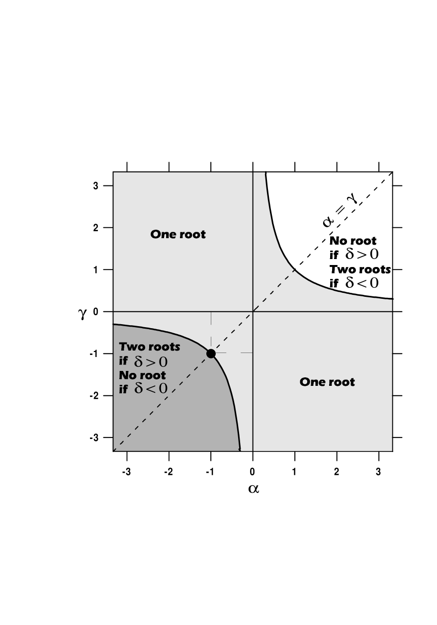
FIG. 1.: The regions in which there are 0, 1 or 2 real positive roots of (8) and hence 0, 1 and 2 bound states.

The $\psi(x)$ and $\psi^{\prime}(x)$ are generally discontinuous at $x=0$ [6, 7]. We obtain the ratio

$$\eta\equiv\frac{\psi(+0)}{\psi(-0)}=\frac{C_{+}}{C_{-}}=-e^{i\theta}\left(\alpha+\frac{2\beta m}{\kappa}\right)=e^{i\theta}\left(\gamma+\frac{\delta\kappa}{2m}\right).$$ (11)

It can be shown that $|\eta|=|\psi(+0)/\psi(-0)|=1$ if and only if $\alpha=\gamma$.

Let us consider the case in which there are two bound states. It is understood that $\delta\neq 0$. In this case the ratio of (11) can be reduced to

$$\eta=-\frac{1}{2}e^{i\theta}\left[\alpha-\gamma\mp\sqrt{(\alpha-\gamma)^{2}+4\,}\,\right]\,.$$ (12)

If we distinguish the $C_{\pm}$’s of the two bound states by adding superscripts $(\pm)$ that correspond to the $\pm$ of (9) and (10) or the $\mp$ of (12), we obtain

$$C^{*(+)}_{+}C^{(-)}_{+}+C^{*(+)}_{-}C^{(-)}_{-}=0\,.$$ (13)

By using this relation one can show that the wave functions of the two bound states are orthogonal to each other.

Let us look into the special case of $\alpha=\gamma$ and $\delta\neq 0$. In this case we obtain

$$\eta=\pm e^{i\theta}\,,$$ (14)

where the double sign corresponds to those of (9) and (10). Suppose we choose $\theta$ as $e^{i\theta}=1$. If there are two bound states, as we discussed below (10), the parity is even for the ground state and odd for the excited state. If we choose $\theta$ as $e^{i\theta}=-1$, the parity of each of the states is reversed. We will discuss this aspect more in appendix 1.

In addition to the bound state problem, the problem of transmission and reflection can also be worked out [6, 7]. We will quote the transmission and reflection coefficients in section 4 where we will examine the three-body scattering problem.

Before proceeding to the three-body and many-body systems that we examine in the next section, it would be useful to briefly examine the two-body system. Let us introduce the variable $x$ defined by

$$x=\frac{1}{\sqrt{2}}(x_{1}-x_{2})\,.$$ (15)

This $x$ differs from the usual relative coordinate by a factor of $\sqrt{2}$. We use this because this is one of the Jacobi coordinates that are commonly used in the three-body problem. In this way we are treating the two-body system as a subsystem of a three-body system. The centre-of-mass coordinate can be separated as usual and the Schrödinger equation for the system can be reduced to

$$\left[-\frac{1}{2m}\frac{d^{2}}{dx^{2}}+V(x)\right]\psi(x)=E\psi(x)\,,$$ (16)

where $V(x)$ stands for the point interaction that is defined by the boundary condition (1) together with (2). The energy $E$ does not contain the part that is due to the centre-of-mass motion.

The interaction $V(x)$ of (16) can be a source of confusion. Recall that the inter-particle distance is $x_{1}-x_{2}=\sqrt{2}x$. To make the problem clear, let us consider the usual $\delta$-function potential. Suppose that we start with the two-body interaction $V(x_{1}-x_{2})=g_{0}\delta(x_{1}-x_{2})$ and change the variable to $x$, we obtain $V(x_{1}-x_{2})=g_{0}\delta(\sqrt{2}x)=(g_{0}/\sqrt{2})\delta(x)$. In this interpretation, the interaction of (16) should be $V(\sqrt{2}x)$ rather than $V(x)$. In this connection, see appendix 2. For a generalized interaction, the boundary condition of (1) has to be appropriately scaled.

In this paper we take a different interpretation. Instead of starting with $V(x_{1}-x_{2})$ and scaling the interaction and the boundary condition as we described above, let us take the $V(x)$ of (16) as the one defined by (1) and (2) with the understanding that $x$ is the variable defined by (15). After all we take this as a matter of definition of the two-body interaction. The main issue that we want to focus on is, with the two-body interaction so defined, how the three-body problem can be solved. A great advantage of this definition of $V(x)$ of (16) is that all the formulae that we have obtained for the one-body problem can be used for the two-body and many-body problems with the understanding that $x$ is the one defined by (15). For a bound state of the two-particle system, the wave function is given by (6) and its energy by (7), and so on.

III Three-body and many-body bound states

We consider a system of many particles of equal masses, interacting through a point interaction that is represented by boundary condition (1). We begin with the three-body problem. Let the coordinates of the three particles be $x_{1}$, $x_{2}$ and $x_{3}$, and introduce the Jacobi coordinates $x$, $y$ and $z$ by

$$x=\frac{1}{\sqrt{2}}(x_{1}-x_{2})\,,\;\;\;y=\sqrt{\frac{2}{3}}\left(\frac{x_{1}+x_{2}}{2}-x_{3}\right),$$ (17)

$$z=\frac{1}{\sqrt{3}}(x_{1}+x_{2}+x_{3})\,.$$ (18)

$$\frac{x-\sqrt{3}y}{2}=\frac{-(x_{2}-x_{3})}{\sqrt{2}}\,,\;\frac{x+\sqrt{3}y}{2}=\frac{-(x_{3}-x_{1})}{\sqrt{2}}\,.$$ (19)

The Schrödinger equation for the three-body system reads

$$\left[-\frac{1}{2m}\left(\frac{\partial^{2}}{\partial x^{2}}+\frac{\partial^{2}}{\partial y^{2}}\right)+V(x)+V\left(-\frac{x-\sqrt{3}y}{2}\right)\right.$$ (20)

$$\left.+V\left(-\frac{x+\sqrt{3}y}{2}\right)\right]\psi(x,y)=E\psi(x,y)\,.$$ (21)

It is understood that the coordinate $z$ (that is essentially the centre-of mass coordinate) has been separated already. It is also understood that the two-body interactions like $V(x)$ are interpreted as in section 2, below (14).

Let us consider six regions that are specified in terms of the signs of $x_{12}$, $x_{23}$ and $x_{31}$, where $x_{ij}=(x_{i}-x_{j})/\sqrt{2}$.  We designate the regions with 1, 2, $\cdots$ , 6, or with $(++-)$, $(-+-)$, $\cdots$ , $(+--)$; see figure 2. For example, in region 1, $x_{12}>0$, $x_{23}>0$ and $x_{31}<0$. Note that $(+++)$ and $(---)$ are not possible. Our six regions 1, 2, $\cdots$ , 6 correspond to McGuire’s regions II, I, III, V, VI and IV, in this order.

Let us assume that the interaction is effectively attractive and there is a bound state. In each of the six regions, the Schrödinger equation for the three-particle system is satisfied by

$$\phi(x,y)=e^{-\kappa\left(|x|+\frac{|x+\sqrt{3}y|}{2}+\frac{|x-\sqrt{3}y|}{2}\right)},$$ (22)

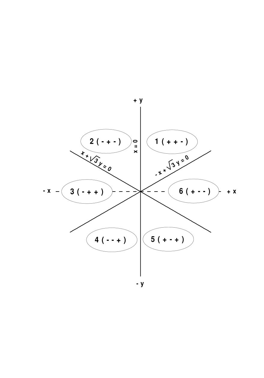
FIG. 2.: Six regions 1,2, $\cdots$, 6 of the three-particle configuration that are divided by three lines $x_{12}=0,\;x_{23}=0$ and $x_{31}=0$. In this connection, see (15) and (16). The order of entries in $(++-)$ etc. refer to the signs of $x_{12},\;x_{23}$ and $x_{31}$, respectively.

where $\kappa>0$ is a constant that is to be determined. The $\phi(x,y)$ is totally symmetric with respect to the interchange of any pair of particles 1, 2 and 3. Let us assume that the wave function of the bound state in each of the regions is of the form of

$$\psi_{\nu}(x,y)=C_{\nu}\phi(x,y)\,,\;\;\;\nu=1,2,\cdots,6\,.$$ (23)

The energy $E$ of the bound state is given by

$$E=-\frac{2\kappa^{2}}{m}\,.$$ (24)

In order to satisfy the Schrödinger equation in the entire space, the wave function has to satisfy the boundary conditions at $x=0$, etc. where the point interactions act. This can be done as follows. Let us start with region 1 by assuming the wave function $\psi_{1}(x,y)=C_{1}\phi(x,y)$ and apply the boundary condition (1) to determine the wave function in region 2. In doing so, we do not have to be concerned with the $y$-dependence of the wave function. In the vicinity of the line $x=0$, the Schrödinger equation (21) can essentially be reduced to the two-particle equation (16). Note that in going from region 1 to region 2, $x$ changes from positive to negative. See, the signs of $x_{12}=(x_{1}-x_{2})/\sqrt{2}$, $x_{23}$ and $x_{31}$ shown in figure 2. We thus obtain

$$C_{2}=\frac{C_{1}}{\eta},$$ (25)

where $\eta$ is given by (11). The $\kappa$ that appears in $\eta$ is that of (9), the same $\kappa$ as that of the two-body case.

Next let us turn to the relation between $C_{2}$ and $C_{3}$. It is convenient to introduce another set of Jacobi coordinates $x^{\prime}$, $y^{\prime}$ and $z^{\prime}$, which are respectively defined in terms of $x$, $y$ and $z$ of (18) in which $x_{1}$, $x_{2}$ and $x_{3}$ are replaced by $x_{3}$, $x_{1}$ and $x_{2}$. Then the line that separates regions 2 and 3 is represented by $x^{\prime}=0$. We start in region 2 with the wave function $C_{2}\phi(x^{\prime},y^{\prime})$. Recall that $\phi(x,y)=\phi(x^{\prime},y^{\prime})$, which is totally symmetric as we stated below (22). The boundary condition along $x^{\prime}=0$ leads to the wave function $C_{3}\phi(x^{\prime},y^{\prime})$ of region 3 where $C_{3}=\eta C_{2}=C_{1}$. The reason why we obtain the factor $\eta$ rather than $1/\eta$ as in (25) is that, in going from region 2 to region 3, $x^{\prime}$ changes from negative to positive. Repeating similar steps we arrive at

$$C_{1}=C_{3}=C_{5}\,,\hskip 11.38092ptC_{2}=C_{4}=C_{6}=\frac{C_{1}}{\eta}\,.$$ (26)

If there are two possible values of $\kappa$, there are two bound states of the three-body system. For the coefficients $C_{\nu}$’s of the two bound states, a relation of the form of (13) holds for any two adjacent regions like 1 and 2. This leads to the orthogonality between the two states.

The $\kappa$ and hence the energy of the bound state is independent of $\theta$. The probability distribution $|\psi_{\nu}(x,y)|^{2}$ is also independent of $\theta$. The wave function and the energy are both smooth functions of the parameters of the interaction. Start with arbitrary values of the parameters. Let them continuously vary and approach the values of (4), then we obtain McGuire’s results for the $\delta$-function potential. Let us assume that no level crossing takes place in this limiting procedure. In the limit of the $\delta$-function potential we know that there can be only one bound state. It then follows that the bound state with the lower energy that we have obtained above is the ground state.

If $\alpha=\gamma$ and $e^{i\theta}=1$, then $\eta=1$. The ground state is totally symmetric with respect to interchanges of the particles. The excited state, if it exists as we discussed below (11), is totally antisymmetric. If $\alpha=\gamma$, and $e^{i\theta}=-1$, the symmetry and antisymmetry of the two states are reversed.

Next let us consider the $N$-particle system. There are $N$! linear configurations of the $N$ particles. Assume that the wave function is of the form of

$$\psi_{\nu}=C_{\nu}\exp(-\kappa\sum_{i>j}|x_{ij}|)\,,\;\;\;x_{ij}=\frac{1}{\sqrt{2}}(x_{i}-x_{j})\,,$$ (27)

where $\nu$ refers to one of the $N$! configurations and $C_{\nu}$ is a constant coefficient associated with configuration $\nu$. It is understood that the centre-of-mass coordinate has been separated. Start with the configuration (1,2,3, $\cdots$ , $N$), for example, and proceed to (2,1,3, $\cdots$, $N$). Along the boundary between these two configurations, the $N$-particle Schrödinger equation is again reduced to the two-particle equation (16). Therefore the coefficient $C_{2}$ can be related to $C_{1}$ exactly in the same way as in (25), with the $\kappa$ of (9). When we go from one configuration to another, factor $\eta$ or $1/\eta$ enters for every permutation. The configurations can be grouped into those of even and odd permutations. The $C_{\nu}$’s are equal within each of the two groups. The $C_{\nu}$’s of different groups differ by factor $\eta$. Starting with the initial configuration, another configuration can be reached in different ways, but this does not give rise to any ambiguity in determining $C_{\nu}$’s. For the nomalization of wave functions of the form of (27), see [11].

The energy of the bound state is given by

$$E=-\frac{\kappa^{2}}{12m}N(N^{2}-1)\,,$$ (28)

where $\kappa$ is again that of (9). There can be two bound states. The $N$-dependence of $E$ is the same as that for the $\delta$-function potential. For the derivation of the $N$-dependent factor, see the appendix of McGuire’s paper [1].

IV Scattering states

McGuire showed how the scattering or the transmission and reflection problem for many-particle systems can be solved exactly for the $\delta$-function potential [1]. In this section let us examine the three-particle case. If the three-particle case can be solved, many-body cases can be done in a similar manner as shown by McGuire. The three-particle system can be regarded as one particle in two dimensions, as can be seen from (21). A wave propagates in the $x$-$y$ plane and meets the interactions along the three lines $x=0$, etc. For the solvability of the problem à la McGuire, it is crucial that there is no diffraction. As McGuire showed, indeed there is no diffraction when the interaction is the $\delta$-function potential. For the general point interactions, however, there is diffraction. This means that unfortunately McGuire’s method as such does not work. This is what we are going to show below.

We will not review McGuire’s calculation. Rather we simply apply it to the present case. Consider a ray (or a wave) incident in region 2 and transmitted and reflected by the potential barriers. Let us focus on the ray that goes out into region 1. There are two geometries as shown in figures 3 and 4.

Assume that the amplitude of the incident wave is unity. In figure 3, the ray that goes through points A, B and A^′ obtains amplitude $T_{1-}R_{2+}R_{3+}$ and the other route of A, C and A^′ leads to $R_{1-}R_{2-}T_{3-}$ . In figure 4, the amplitude of the outgoing ray is $R_{3-}T_{2+}R_{1+}$. Here the $T$’s and $R$’s are the transmission and reflection coefficients that have been worked out before [6, 7]; we give them explicitly below. The suffices $+$ and $-$ indicate the direction of incidence, which were respectively denoted with R and L before. Suffices 1, 2 and 3 refer to the three angles of incidence,

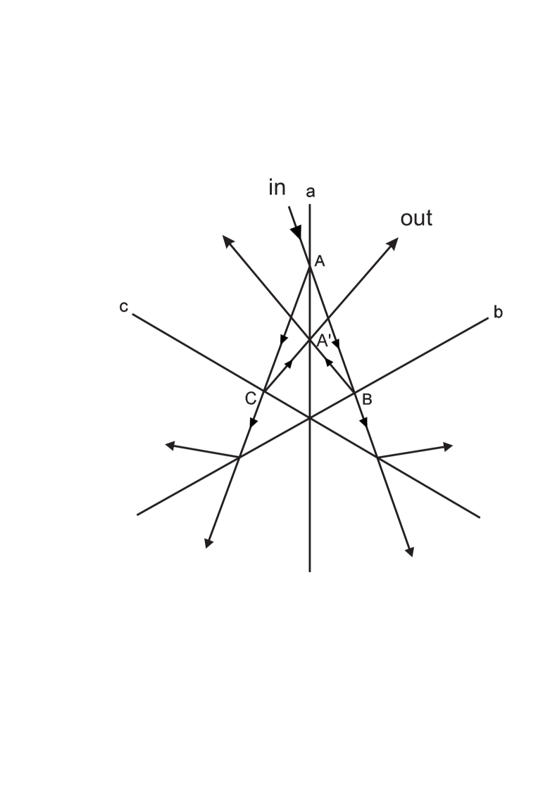
FIG. 3.: Ray diagram that applies when the incoming hits the potential line $x=0\;$ i.e. $x_{12}=0$ first. We focus on the ray that is incident in region 2 and goes out in region 1. For the regions, see figure 2.

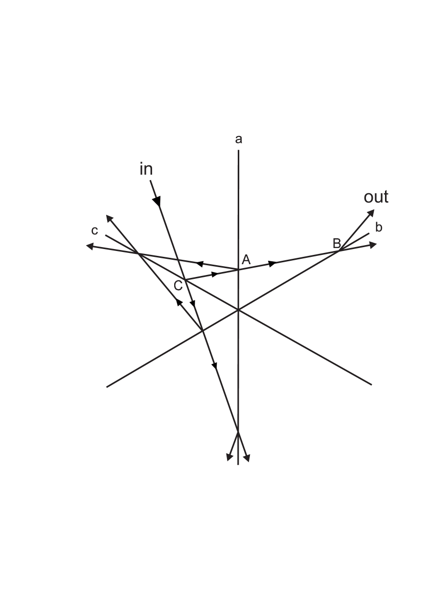
FIG. 4.: Ray diagram that applies when the incoming hits the potential line $(x+\sqrt{3}y)=0\;$ i.e. $x_{31}=0$ first. We focus on the ray that is incident in region 2 and goes out in region 1. For the regions, see figure 2.

$$\varphi_{1}=\varphi\,,\;\;\;\varphi_{2}=\varphi+\frac{\pi}{3}\,,\;\;\;\varphi_{3}=-\varphi+\frac{\pi}{3}\,,\;\;\;$$ (29)

which were defined by McGuire [1]. The $T_{i\pm}$ and $R_{i\pm}$ are associated with the normal components of $k$,

$$k_{i}=k\sin\varphi_{i}\,,\;\;\;i=1,2,3\,.$$ (30)

Note that

$$k_{1}+k_{2}=k_{3}\,.$$ (31)

The path lengths of the rays in the two geometries are equal. If the two amplitudes associated with the outgoing rays that are shown in figures 3 and 4, i.e.,

$$R_{1-}R_{2-}T_{3-}+T_{1-}R_{2-}R_{3+}\;\;\;{\rm and}\;\;\;R_{3-}T_{2+}R_{1+}\;,$$ (32)

are equal, there is no diffraction. Then the wave function of the scattering state can be written down as was done by McGuire. This was indeed the case for the $\delta$-function potential. In that case the relation (31) is instrumental.

For the point interactions of the four-parameter family, the $T$’s and $R$’s read as [6, 7],

$$T_{\pm}=\frac{4ie^{\mp i\theta}km}{D}\,,$$ (33)

$$R_{\pm}=\frac{\delta k^{2}\mp 2ikm(\alpha-\gamma)+4\beta m^{2}}{D}\,,$$ (34)

$$D=\delta k^{2}+2ikm(\alpha+\gamma)-4\beta m^{2}\,.$$ (35)

Note that $T_{+}\neq T_{-}$ unless $e^{i\theta}$ is real. The $R_{\pm}$ are independent of $\theta$. Although somewhat tedious it is straightforward to show that the condition for vanishing diffraction can be satisfied for arbitrary $k$ and $\varphi$ if and only if

$$\alpha=\gamma\,,\;\;\;\delta=0\,,\;\;\;e^{i\theta}=\pm 1\,.$$ (36)

If we combine (36) with the constraint $\alpha\gamma-\beta\delta=1$, we obtain $\alpha=\gamma=\pm 1$. It is interesting that ADF [7] arrived at exactly the same condition by examining the Yang-Baxter equation for the system within the context of the Bethe ansatz [2, 12].

If $e^{i\theta}=-1$, the interaction of $\alpha=\gamma=-1$ is the usual $\delta$-function potential of (5) and we obtain McGuire’s solution. The other interaction of $\alpha=\gamma=1$, which ADF called the “anti-$\delta$ interaction”, differs from the $\delta$-function potential only through the different choice of $e^{i\theta}$. For these two interactions, the wave functions of the three-body system only differ in the sign that depends on the six regions; the scattering amplitudes of (32) differ only through their overall sign. For the physical quantities of the system, the two interactions end up with identical results. In this sense they are essentially equivalent. See, however, appendix 1.

V Summary and Discussion

We have attempted to extend McGuire’s work [1] on the many-particle system interacting through the $\delta$-function potential to accommodate the four-parameter family of point interactions. We have succeeded in doing so for the bound states, but not quite for the scattering states. For the bound states we obtained exact solutions. If the interaction supports one or two bound states for the two-body system, it supports the same number of bound states for an $N$-body system. It is interesting that, unlike McGuire’s case, there can be two bound states (for the same system with the same interaction). We suspect that what we have found exhausts all possible bound states, but we have no rigorous proof for that.

The scattering problem becomes complicated in general because of the emergence of diffraction. McGuire’s method as such does not work unless the parameters are restricted to (36). There is no such restriction in the bound state problem. The condition of no diffraction is instrumental for the scattering problem but it is not for the bound state. We admit that we were surprised by this finding. The emergence of diffraction does not necessarily mean the nonexistence of scattering solutions. We believe that scattering solutions exist even in the presence of diffraction. The solutions would require more sophisticated approach, probably, such as those developed by Albeverio, McGuire and Hurst, and Lipszyc [13]. In the cases that were examined in [13] diffraction occurs because the particles have different masses, or the interactions for different pairs are different, and so on. Still scattering solutions can be constructed.

ADF [7] independently examined essentially the same problem as what we have done except that they also considered the impenetrable type of point interactions that we have not considered. Let us comment only on their results on the penetrable type. For the scattering problem, ADF’s results and ours agree. For the bound state problem, ADF obtained solutions only for the parameter sets for which they found scattering solutions. As we emphasized already, the bound solutions that we found have no such restrictions. ADF’s solutions are special cases of our solutions. As we said above there can be two bound states. ADF’s solutions have no such possibility.

REFERENCES

- [1] McGuire J B 1964 J. Math. Phys. 5 622; 1965 ibid 6 432
- [2] Yang C N 1967 Phys. Rev. Lett. 19 1312; 1968 Phys. Rev. 168 1920
- [3] Albeverio S, Gesztesy F, Hegh-Krohn R and Holden H 1988 Solvable Models in Quantum Mechanics (Berlin: Springer)
- [4] Šeba P 1986 Czech. J. Phys. B 36 667; 1986 Rep. Math. Phys. 24 111
- [5] Gesztesy F and Holden H 1987 J. Phys. A: Math. Gen. 20 5157
- [6] Chernoff P R and Hughes R J 1993 J. Functional Analysis 111 97
- [7] Coutinho F A B, Nogami Y and Perez J F 1997 J. Phys. A: Math. Gen. 30 3937 (1997) and earlier references quoted there
- [8] Coutinho F A B, Nogami Y and Perez J F 1998 Time-reversal aspect of the point interactions in one-dimensional quantum mechanics J. Phys. A: Math. Gen. in press
- [9] Albeverio S, Da̧browski L and Fei S-M 1998 One dimensional many-body problems with point interactions SISSA 139/FM/98
- [10] Albeverio S, Da̧browski L and Kurasov P 1998 Lett. Math. Phys. 45 33
- [11] Calogero F and Degasperis A 1975 Phys. Rev. A 11 265
- [12] Baxter R J 1972 Ann. Phys. 70 193; 1978 Phil. Trans. Royal Soc. London 289 315
-
[13]
Albeverio S 1969 Helv. Phys. Acta 40 135;
McGuire J B and Hurst C A 1972 J. Math. Phys. 13 1595;
Lipszyc K 1972 Acta Phys. Pol. A 42 571; 1974 J. Math. Phys. 15 133; 1980 J. Math. Phys. 21 1092
Appendix 1: Symmetry of the bound state wave functions
In this appendix we assume . Let us consider the bound states of the one-particle system that we discussed in section 2, in particular, the case of and . Since , the system is invariant under space reflection, and parity is a good quantum number. Assume so that there are two bound states.
As we pointed out in section 2, if the parity is even for the ground state and is odd for the excited state. On the other hand, if the parity is odd for the ground state and is even for the excited state. This may sound odd but there is nothing wrong with this in principle.
Let us consider an -body system with the same interactions assumed above. If there are two bound states in the two-body case, there are also two bound states in the -body case. If , the ground state is totally symmetric and the excited state totally antisymmetric. If , the symmetry and antisymmetry of the two states are reversed. A totally symmetric (antisymmetric) state can accommodate bosons (fermions). There is “duality” between the boson systems. All physically observable quantities are the same between the two systems.
Let us add that, with , the wave function of a bound state for an attractive interaction is of the same form as that of an attractive -function potential. This may seem to imply a kind of duality. The and interactions, however, give different transmission and reflection coefficients. In this sense this duality is restricted to bound states.
Appendix 2: The -function potential
In order to facilitate comparison between our results and those of McGuire [1], let us summarize the case in which we start with the two-particle interaction