The Hidden Subgroup Problem and Eigenvalue Estimation on a Quantum Computer

Abstract

A quantum computer can efficiently find the order of an element in a group, factors of composite integers, discrete logarithms, stabilisers in Abelian groups, and hidden or unknown subgroups of Abelian groups. It is already known how to phrase the first four problems as the estimation of eigenvalues of certain unitary operators. Here we show how the solution to the more general Abelian hidden subgroup problem can also be described and analysed as such. We then point out how certain instances of these problems can be solved with only one control qubit, or flying qubits, instead of entire registers of control qubits.

1 Introduction

Shor’s approach to factoring [Sh], (by finding the order of elements in the multiplicative group of integers mod $N$, referred to as ${\mathbf{Z}}_{N}^{*}$) is to extract the period in a superposition by applying a Fourier transform. Another approach, based on Kitaev’s technique [Ki], is to estimate an eigenvalue of a certain unitary operator. The difference between the two analyses is that the first one considers (or even ’measures’ or ’observes’) the target or output register in the standard computational basis, while the analysis we detail here considers the target register in a basis containing eigenvectors of unitary operators related to the function $f$. The actual network of quantum gates, as highlighted in [CEMM], is the same for both algorithms; it is helpful to understand both approaches. In some cases, which we discuss in Sect. 5, this approach suggests implementations which do not require a register of control qubits. A more general formulation of the order-finding problem as well as the discrete logarithm problem, and the Abelian stabiliser problem, is the hidden subgroup problem (or the unknown subgroup problem [Hø]). In the case that $G$ is presented as the product of a finite number of cyclic groups (so $G$ is finitely generated and Abelian), all of these problems are solved by the familiar sequence of a Fourier transform, a function application, and an inverse Fourier transform. In this paper we describe how this more general problem can also be viewed and analysed as an estimation of eigenvalues of unitary operators.

2 The Hidden Subgroup Problem

Let $f$ be a function from a finitely generated group $G$ to a finite set $X$ such that $f$ is constant on the cosets of a subgroup $K$ (of finite index, since $X$ is finite), and distinct on each coset. The hidden subgroup problem is to find $K$ (that is, a generating set for $K$), given a way of computing $f$. When $K$ is normal in $G$, we could in fact decompose $f$ as $h\circ g$, where $g$ is a homomorphism from $G$ to some finite group $H$, and $h$ is some 1-to-1 mapping from $H$ to the set $X$. In this case, $K$ corresponds to the kernel of $g$ and $H$ is isomorphic to $G/K$. We will occasionally refer to this decomposition, which we illustrate in Fig. 1.

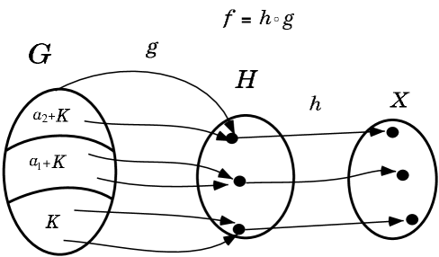
Figure 1: The function $f$ can be viewed as the composition of a homomorphism $g$ to a group $H$, and some 1-to-1 mapping $h$ to the set $X$. Our hidden subgroup $K$ will be the kernel of $g$, and $H$ is isomorphic to $G/K$.

Define the input size, $n$, to be of order $\log_{2}[G:K]$. We will count the number of operations, or the running time, in terms of $n$. An algorithm is considered efficient if its running time is polynomial in the input size. By elementary quantum operations, we are referring to a finite set of quantum logic gates which allow us to approximate any unitary operation. See [BBCDMSSSW] for a discussion and further references. Our running times will always refer to expected running times, unless explicitly stated otherwise. By expected running time we are referring to the expected number of operations for any input (and not just an average of the expected running times over all inputs).

We should be clear about what it means to have a finitely generated group $G$, and to be able to compute the function $f$. This is difficult without losing some generality or being dry and technical, or both. The algorithms we describe only apply for groups $G$ which are represented as finite tuples of integers corresponding to the direct product of cyclic groups (consequently, $G$ is finitely generated and Abelian). Conversely, for any finitely generated Abelian $G$, there is a temptation to point out that $G$ is isomorphic to such a direct product of cyclic groups, and assume that we can easily access this product structure. This is not always the case, even in cases of practical interest. For example, ${\mathbf{Z}}_{N}^{*}$, the multiplicative group of integers modulo $N$ for some large integer $N$, which is Abelian of order $\phi(N)$ (the Euler $\phi$-function) and thus isomorphic to a product of cyclic groups of prime power order. We will not necessarily know $\phi(N)$ or have a factorisation of it along with a set of generators for ${\mathbf{Z}}_{N}^{*}$. However, in light of the quantum algorithms described in this paper, we could efficiently find such an isomorphism, thereby increasing the number of finitely generated Abelian groups which can be efficiently expressed in a manner which allows us to employ these algorithms. We will however leave further discussion of these details to another note [EM]. When we talk about computing $f$, we assume that we have some unitary operation $U_{f}$ which takes us from state $\left|\,\mathbf{x}\right\rangle\left|\,\mathbf{0}\right\rangle$ to $\left|\,\mathbf{x}\right\rangle\left|\,f({\mathbf{x}})\right\rangle$. It could, for example, take $\left|\,\mathbf{x}\right\rangle\left|\,\mathbf{y}\right\rangle$ to $\left|\,\mathbf{x}\right\rangle\left|\,{\mathbf{y}}+f({\mathbf{x}})\right\rangle$, where $+$ denotes an appropriate group operation, such as addition modulo $N$ when the second register is used to represent the integers modulo $N$.

Various cases of the hidden subgroup problem are described in [Si], [Sh], [Ki], [BL], [Gr], [Jo], [CEMM], and [Hø]. We note that [BL] also covers the case that $f$ is not necessarily distinct on each coset (that is, $h$ is not 1-to-1), and this is discussed in the appendix. Finding the order $r$ of an element in a group $H$ of unknown size, or the period $r$ of a function $f$, is a special case where $G={\mathbf{Z}}$ and $K=r{\mathbf{Z}}$. For any generator $\mathbf{e_{j}}$ of a finitely generated $G$, we can use the algorithm in Sect. 4.2 to find an integer $k$ such that $f(k{\mathbf{e_{j}}})=f({\mathbf{0}})$, so that $k{\mathbf{e_{j}}}\in K$. We find this $k$ with $O(n)$ applications of $f$ and $O(n^{2})$ other elementary quantum operations. We can then assume that $\mathbf{e_{j}}$ is of order $k$ (that is, factor $\langle k{\mathbf{e_{j}}}\rangle$ out of $G$), and in general assume that $G$ is a finite group.

We give a few examples.

Deutsch’s Problem: Consider a function $f$ mapping ${\mathbf{Z}}_{2}=\{0,1\}$ to $\{0,1\}$. Then $f(x)=f(y)$ if and only if $x-y\in K$, where where $K$ is either $\{0\}$ or ${\mathbf{Z}}_{2}=\{0,1\}$. If $K$ is $\{0\}$, then $f$ is $1-to-1$ (or balanced), and if $K$ is ${\mathbf{Z}}_{2}$ then $f$ is constant. [De] [CEMM]

Simon’s Problem: Consider a function $f$ from ${{\mathbf{Z}}_{2}}^{l}$ to some set $X$ with the property that $f(x)=f(y)$ if and only if $x-y\in\{\mathbf{0},\mathbf{s}\}$ for some string $\mathbf{s}$ of length $l$. Here $K=\{\mathbf{0},\mathbf{s}\}$ is the hidden subgroup of ${{\mathbf{Z}}_{2}}^{l}$. Simon [Si] presents an efficient algorithm for solving this problem, and the solution to the hidden subgroup problem in the Abelian case is a generalisation.

Discrete Logarithms: Let $G$ be the group ${\mathbf{Z}}_{r}\times{\mathbf{Z}}_{r}$ where ${\mathbf{Z}}_{r}$ is the additive group of integers modulo $r$. Let the set $X$ be the subgroup generated by some element $a$ of a group $H$, with $a^{r}=1$. For example, $H={\mathbf{F}}_{q}^{*}$, the multiplicative group of the field of order $q$, where $r=q-1$. Let $a,b\in G$, and suppose $b=a^{m}$. Define $f$ to map $(x,y)$ to $a^{x}b^{y}$. Here the hidden subgroup of $G$ is $K=\{(k,-km)|k=0,1,\ldots,r-1\}=\langle(1,-m)\rangle$, the subgroup generated by $(1,-m)$. Finding this hidden subgroup will give us the logarithm of $b$ to the base $a$. The security of the U.S. Digital Signature Algorithm is based on the computational difficulty of this problem in ${\mathbf{F}}_{q}^{*}$ (see [MOV] for details and references). Here the input size is $n=\lceil\log_{2}r\rceil$. Shor’s algorithm [Sh] was the first to solve this problem efficiently. In this case, $f$ is also a homomorphism which can make implementations more simple as described in Sect. 5.

Self-Shift-Equivalent Polynomials: Given a polynomial $P$ in $l$ variables $X_{1}$, $X_{2}$, $\ldots,X_{l}$ over ${\mathbf{F}}_{q}$, the function $f$ which maps $(a_{1},a_{2},\ldots,a_{l})\in{\mathbf{F}}_{q}^{l}$ to $P(X_{1}-a_{1},X_{2}-a_{2},\ldots,X_{l}-a_{l})$ is constant on cosets of a subgroup $K$ of ${{\mathbf{F}}_{q}^{l}}$. This subgroup $K$ is the set of self-shift-equivalences of the polynomial $P$. Grigoriev [Gr] shows how to compute this subgroup. He also shows, in the case that $q$ has characteristic $2$, how to decide if two polynomials $P_{1}$ and $P_{2}$ are shift-equivalent, and to generate the set of elements $(a_{1},a_{2},\ldots,a_{l})$ such that $P_{1}(X_{1}-a_{1},X_{2}-a_{2},\ldots,X_{l}-a_{l})=P_{2}(X_{1},X_{2},\ldots,X_{l})$. The input size $n$ is at most $l\log_{2}q$.

Abelian Stabiliser Problem: Let $G$ be any group acting on a finite set $X$. That is, each element of $G$ acts as a map from $X$ to $X$, in such a way that for any two elements $a,b\in G$, $a(b(x))=(ab)(x)$ for all $x\in X$. For a particular element $x$ of $X$, the set of elements which fix $x$ (that is, the elements $a\in G$ such that $a(x)=x$), form a subgroup. This subgroup is called the stabiliser of $x$ in $G$, denoted $St_{G}(x)$. Let $f_{x}$ denote the function from $G$ to $X$ which maps $g\in G$ to $g(x)$. The hidden subgroup corresponding to $f_{x}$ is $K=St_{G}(x)$. The finitely generated Abelian case of this problem was solved by Kitaev [Ki], and includes finding orders and discrete logarithms as special cases.

3 Phase Estimation and the Quantum Fourier Transform

In this section, we review the relationship between phase estimation and the quantum Fourier transform which was highlighted in [CEMM].

The quantum Fourier transform for the cyclic group of order $N$, $F_{N}$, maps

$$\left|\,a\right\rangle\rightarrow{1\over\sqrt{N}}\sum_{x=0}^{N-1}e^{2\pi iax/N}\left|\,x\right\rangle.$$

So $F_{N}^{-1}$ maps

$${1\over\sqrt{N}}\sum_{x=0}^{N-1}e^{2\pi iax/N}\left|\,x\right\rangle\rightarrow\left|\,a\right\rangle.$$

More generally, for any $\phi$, $0\leq\phi<1$, $F_{N}^{-1}$ maps

$${1\over\sqrt{N}}\sum_{x=0}^{N-1}e^{2\pi i{\phi x}}\left|\,x\right\rangle\rightarrow\sum_{x=0}^{N-1}\alpha_{\phi,x}\left|\,x\right\rangle$$ (1)

where the amplitudes $\alpha_{\phi,x}$ are concentrated near values of $x$ such that $x/N$ are good estimates of $\phi$. The closest estimate of $\phi$ will have amplitude at least $4/\pi^{2}$. The probability that $x/N$ will be within $k/N$ of $\phi$ is at least $1-1/(2k-1)$. See [CEMM] for details in the case that $N$ is a power of $2$; the same proof works for any $N$. Thus to estimate $\phi$ such that, with probability at least $1-\epsilon$, the error is less than $1/M$, we should use a control register containing values from $0$ to $N-1$ and apply $F_{N}^{-1}$ for any $N\geq M(1/\epsilon+1)/2$. For example, if we desire an error of at most $1/2^{n}$ with probability at least $1-1/2^{m}$ we could use $N=2^{n+m}$. In practice, it will be best to use the $N$ that corresponds to the group that is easiest to represent and work with in the particular physical realisation of the quantum computer at hand. We expect that this $N$ will be a power of two.

For convenience, we will omit normalising factors in the remainder of this paper. It will also be convenient to have a compact notation for the state on the right hand side of (1) which we consider to be a good estimator for $\left|\,\phi\right\rangle$. So let us refer to this state as $\big{|}\,\widetilde{\phi}\big{\rangle}_{N}$ or just $\big{|}\,\widetilde{\phi}\big{\rangle}$ if the value of $N$ is understood. Lastly, we will use $\mbox{exp}(x)$ to denote $e^{x}$.

4 The Algorithm

To restrict attention from finitely generated groups $G$ to finite groups we need to know how to solve the cyclic case (just one generator), that is, to find the period of a function from $\mathbf{Z}$ to the set $X$. We will first describe how to find the order of an element $a$ in a group $H$, or equivalently, the period of the function $f:t\rightarrow a^{t}$, as Shor [Sh] did for the group $H={\mathbf{Z}}_{N}^{*}$, the multiplicative group of integers modulo $N$. We will then show how to generalise it to find the period of any function $f:{\mathbf{Z}}\rightarrow X$. If $f$ were a homomorphism (so $h$ is an isomorphism of $H$, when $f$ is decomposed as $f=h\circ g$), we would just be finding the order of $f(1)$ in $H$. The difference is that we are showing how to deal with a non-trivial $h$ which hides the homomorphism structure. The details will also help explain how to find hidden subgroups of finite Abelian groups.

4.1 Finding Orders in Groups

We have an element $a$ from a group $H$ and we wish to find the smallest positive integer $r$ such that $a^{r}=1$. The group $H$ is not necessarily Abelian; all that matters is that the subgroup generated by $a$ is Abelian, and this is always true. The idea is to create an operator $U_{a}$ which corresponds to multiplication by $a$ (so it maps $\left|\,y\right\rangle$ to $\left|\,ay\right\rangle$). Since $a^{r}=1$, then $U_{a}^{r}=I$, the identity operator. Hence the eigenvalues of $U_{a}$ are $r$th roots of unity, $exp(2\pi ik/r)$, $k=0,1,\ldots,r-1$. By estimating a random eigenvalue of $U_{a}$, with accuracy $1/2r^{2}$, we can determine the fraction $k/r$. The denominator (with the fraction in lowest terms) will be a factor of $r$. We thus seek to estimate an eigenvalue of $U_{a}$; note that $U_{a}^{r}=U_{a^{r}}$.

For any integer $x$ define $U_{a^{x}}$ to be the operator that maps $\left|\,y\right\rangle$ to $\left|\,a^{x}y\right\rangle$. Define $U_{a^{\mbox{x}}}$ to be the operator which maps $\left|\,x\right\rangle\left|\,y\right\rangle$ to $\left|\,x\right\rangle U_{a^{x}}\left|\,y\right\rangle=\left|\,x\right\rangle\left|\,a^{x}y\right\rangle$. Note that $U_{a^{\mbox{x}}}$ acts on two registers and x is a variable which takes on the value in the first register, while $U_{a^{x}}$ acts on one register and $x$ is fixed. Consider the eigenvectors

$$\left|\,\Psi_{k}\right\rangle=\sum_{t=0}^{r-1}\mbox{exp}(-2\pi ikt/r)\left|\,a^{t}\right\rangle,k=0,1,\ldots,r-1,$$ (2)

of $U_{a^{x}}$ and respective eigenvalues $\mbox{exp}(2\pi ikx/r)$ . If we start with the superposition

$$\sum_{x=0}^{2^{l}-1}\left|\,x\right\rangle\left|\,\Psi_{k}\right\rangle$$

and then apply $U_{a^{\mbox{x}}}$ we get

$$\sum_{x=0}^{2^{l}-1}\mbox{exp}(2\pi ikx/r)\left|\,x\right\rangle\left|\,\Psi_{k}\right\rangle.$$

As discussed in the previous section, applying $F_{2^{l}}^{-1}$ to the first register gives $\big{|}\,\widetilde{k/r}\big{\rangle}\left|\,\Psi_{k}\right\rangle$ and thus a good estimate of $k/r$.

We will not typically have $\left|\,\Psi_{k}\right\rangle$ but we do know that $\left|\,1\right\rangle=\sum_{k=0}^{r}\left|\,\Psi_{k}\right\rangle$. Therefore we can start with

$$\left|\,0\right\rangle\left|\,1\right\rangle=\left|\,0\right\rangle\sum_{k=0}^{r}\left|\,\Psi_{k}\right\rangle=\sum_{k=0}^{r}\left|\,0\right\rangle\left|\,\Psi_{k}\right\rangle$$ (3)

and then apply $F_{2^{l}}$ to the first register to produce

$$\sum_{k=0}^{r-1}\left(\sum_{x=0}^{2^{l}-1}\left|\,x\right\rangle\right)\left|\,\Psi_{k}\right\rangle.$$ (4)

We then apply $U_{a^{\mbox{x}}}$ to get

$$\sum_{k=0}^{r-1}\left(\sum_{x=0}^{2^{l}-1}\mbox{exp}(2\pi ikx/r)\left|\,x\right\rangle\right)\left|\,\Psi_{k}\right\rangle$$ (5)

followed by $F_{2^{l}}^{-1}$ on the control register to yield

$$\sum_{k=0}^{r-1}\big{|}\,\widetilde{k/r}\big{\rangle}\left|\,\Psi_{k}\right\rangle.$$ (6)

Observing the first register will give an estimate of $k/r$ for an integer $k$ chosen uniformly at random from the set $\{0,1,\ldots,r-1\}$. As shown in [Sh], we choose $l>2\log_{2}r$, and use the continued fractions algorithm to find the fraction $k/r$. Of course, we do not know $r$, so we must either use an $l$ we know will be larger than $2\log_{2}r$, such as $2\log_{2}N$ in the case that $H$ is $\mathbf{Z}_{N}^{*}$. (Alternatively, we could guess a lower bound for $r$, and if the algorithm fails, subsequently double the guess and repeat.) We then repeat $O(1)$ times to find $r$. This algorithm thus uses $O(1)$ exponentiations, or $O(n)$ group multiplications, and $O(n^{2})$ elementary quantum operations to do the Fourier transforms.

We can factor the integer $N$ by finding orders of elements in ${\mathbf{Z}}_{N}^{*}$. This uses only $O(n^{3})$ or $\mbox{exp}(c\log n)$ elementary quantum operations, for $c=3+o(1)$ (or $c=2+o(1)$ if we use fast Fourier transform techniques). Other deterministic factoring methods will factor $N$ in $O(\sqrt{N})$ or $\mbox{exp}(cn)$ steps, where $c=1/2+o(1)$. The best known rigorous probabilistic classical algorithm (using index calculus methods) [LP] uses $\mbox{exp}(c(n\log{n})^{1/2})$ elementary classical operations, $c=1+o(1)$. There is also an algorithm with a heuristic expected running time of $\mbox{exp}(c(n^{1/3}(\log{n})^{2/3})$ elementary classical operations (see [MOV] for an overview and references) for $c=1.902+o(1)$. Thus, in terms of elementary operations, a quantum computer provides a drastic improvement over known classical methods to factor integers.

4.2 Finding the Period of a Function

The above algorithm, as pointed out in [BL], can be applied to a more general setting. Replace the mapping from $t$ to $a^{t}$ with any function $f$ from the integers to some finite set $X$. Define $U_{f(x)}$ to be an operator that maps $f(y)$ to $f(y+x)$. This is a generalisation of $U_{a^{x}}$ except it does not matter how it is defined on values not in the range of $f$, as long as it is unitary. Define $U_{f(\mbox{x})}$ to be an operator which maps $\left|\,x\right\rangle\left|\,f(y)\right\rangle$ to $\left|\,x\right\rangle U_{f(x)}\left|\,f(y)\right\rangle=\left|\,x\right\rangle\left|\,f(y+x)\right\rangle$.

The following are eigenvectors of $U_{f(x)}$:

$$\left|\,\Psi_{k}\right\rangle=\sum_{t=0}^{r-1}\mbox{exp}(-2\pi ikt/r)\left|\,f(t)\right\rangle,k=0,1,\ldots,r-1,$$ (7)

with respective eigenvalues $\mbox{exp}(2\pi ikx/r)$. As in (3), we can start with

$$\left|\,0\right\rangle\left|\,f(0)\right\rangle=\sum_{k=0}^{r-1}\left|\,0\right\rangle\left|\,\Psi_{k}\right\rangle$$

except with our new, more general, definition of $\left|\,\Psi_{k}\right\rangle$. We apply $F_{2^{n}}$ to the first register to produce (4), and then apply $U_{f(\mbox{x})}$ to produce (5), followed by $F_{2^{n}}^{-1}$ to get (6). Observing the first register will give an estimate of $k/r$ for an integer $k$ chosen uniformly at random, and the same analysis as in the previous section applies to find $r$.

One important issue is how to compute $U_{f(\mbox{x})}$ only knowing how to compute $f$. Note that from (4) to (5) (using the modified definition of $\left|\,\Psi_{k}\right\rangle$) we simply go from

$$\sum_{x=0}^{2^{n}-1}\left|\,x\right\rangle\left|\,f(0)\right\rangle=\sum_{x=0}^{2^{n}-1}\left(\sum_{k=0}^{r-1}\left|\,x\right\rangle\left|\,\Psi_{k}\right\rangle\right)$$ (8)

to

$$\sum_{x=0}^{2^{n}-1}\left|\,x\right\rangle\left|\,f(x)\right\rangle=\sum_{x=0}^{2^{n}-1}\left|\,x\right\rangle\left(\sum_{k=0}^{r-1}\mbox{exp}(2\pi ixk/r)\left|\,\Psi_{k}\right\rangle\right)$$ (9)

which could be accomplished by applying $U_{f}$, which we do have, to the starting state

$$\sum_{x=0}^{2^{n}-1}\left|\,x\right\rangle\left|\,0\right\rangle.$$

Thus even if we do not know how to explicitly compute the operators $U_{f(x)}$, any operator $U_{f}$ which computes the function $f$ will give us the state (9). This state permits us to estimate an eigenvalue of $U_{f(x)}$ which lets us find the period of the function $f$ with just $O(1)$ applications of the operator $U_{f}$ and $O(n^{2})$ other elementary operations. The equality in (9) is the key to the equivalence between the two approaches to these quantum algorithms. On the left hand side is the original approach ([Si], [Sh], [BL]) which considers the target register in the standard computational basis. We can analyse the Fourier transform of the preimages of these basis states, which is less easy when the Fourier transforms do not exactly correspond to the group $G$. On the right hand side of (9) we consider the target register in a basis containing the eigenvectors of the unitary operators which we apply to it (as done in [Ki] and [CEMM], for example), and this gives us (5), from which it is easy to see and analyse the effect of the inverse Fourier transform even when it does not perfectly match the size of $G$.

4.3 Finding Hidden Subgroups

As discussed in Sect. 2, any finite Abelian group $G$ is the product of cyclic groups. In light of the order-finding algorithm, which also permits us to factor, we can assume that the group $G$ is represented as a product of cyclic groups of prime power order. Further, for any product of two groups $G_{p}$ and $G_{q}$ whose orders are coprime, any subgroup $K$ of $G_{p}\times G_{q}$ must be equal to $K_{p}\times K_{q}$ from some subgroups $K_{p}$ and $K_{q}$ of $G_{p}$ and $G_{q}$ respectively. We can therefore consider our function $f$ separately on $G_{p}$ and $G_{q}$ and determine $K_{p}$ and $K_{q}$ separately. Thus we can further restrict ourselves to groups $G$ of prime power order. This not only simplifies any analysis, it could reduce the size of quantum control registers necessary in any implementation of these algorithms.

Let us thus assume that $G={\mathbf{Z}}_{p^{m_{1}}}\times{\mathbf{Z}}_{p^{m_{2}}}\times\cdots\times{\mathbf{Z}}_{p^{m_{l}}}$ for some prime $p$ and positive integers $m_{1}\leq m_{2}\leq\cdots\leq m_{l}=m$. The ‘promise’ is that $f$ is constant on cosets of a subgroup $K$, and distinct on each coset. The hidden subgroup $K$ is $\{{\mathbf{k}}=(k_{1},k_{2},\ldots,k_{l})|f({\mathbf{x}})=f({\mathbf{x}}+{\mathbf{k}})\hskip 5.69054pt\mbox{ for all }\hskip 5.69054pt{\mathbf{x}}\in G\}$. In practice, this will usually be a consequence of the nature of $f$, as in the case of discrete logarithms where $f(x_{1},x_{2})=a^{x_{1}}b^{x_{2}}$, or whenever $f$ is constructed as $h\circ g$ for some homomorphism $g$ from $G$ to some finite group $H$, and a 1-to-1 mapping $h$ from $H$ to the set $X$.

Let $U_{f}$ be an operator which maps $\left|\,\mathbf{x}\right\rangle\left|\,\mathbf{0}\right\rangle$ to $\left|\,\mathbf{x}\right\rangle\left|\,f(\mathbf{x})\right\rangle$. Define ${\mathbf{e_{1}}}=(1,0,\ldots,0)$, ${\mathbf{e_{2}}}=(0,1,0,\ldots,0)$, and so on. Let us also consider an operator related to $U_{f}$, $U_{f(\mbox{x}{\mathbf{e_{j}}})}$, which maps $\left|\,x\right\rangle\left|\,f(\mathbf{y})\right\rangle$ to $\left|\,x\right\rangle U_{f(x{\mathbf{e_{j}}})}\left|\,f(\mathbf{y})\right\rangle=\left|\,x\right\rangle\left|\,f({\mathbf{y}}+x{\mathbf{e_{j}}})\right\rangle$. In the case of Simon’s Problem, the operator $U_{f(\mbox{x}(0,1,0))}$ maps $\left|\,1\right\rangle\left|\,f(y_{1},y_{2},y_{3})\right\rangle$ to $\left|\,1\right\rangle U_{f(0,1,0)}\left|\,f(y_{1},y_{2},y_{3}))\right\rangle$ $=\left|\,1\right\rangle\left|\,f(y_{1},y_{2}+1,y_{3})\right\rangle$ and does nothing to $\left|\,0\right\rangle\left|\,f(y_{1},y_{2},y_{3})\right\rangle$.

For each ${\mathbf{t}}=(t_{1},t_{2},\ldots,t_{l})$, $0\leq t_{j}<p^{m_{j}}$, satisfying

$$\sum_{j=1}^{l}{p^{m-m_{j}}h_{j}t_{j}}=0\mbox{ mod }p^{m}\hskip 5.69054pt\mbox{ for all }{\mathbf{h}}\in K$$ (10)

define

$$\left|\,\Psi_{\mathbf{t}}\right\rangle=\sum_{\mathbf{a}\in G/K}\mbox{exp}\left({-2\pi i\over p^{m}}\sum_{j=1}^{l}{p^{m-m_{j}}t_{j}a_{j}}\right)\left|\,f(\mathbf{a})\right\rangle.$$ (11)

We are summing over a set of representatives of the cosets of $K$ modulo $G$, and by condition (10) on $\mathbf{t}$, this sum is well-defined. Let $T$ denote the set of $\mathbf{t}$ satisfying (10), which corresponds to the group of characters of $G/K$. The $\left|\,\Psi_{\mathbf{t}}\right\rangle$ are eigenvectors of each $U_{f(x\mathbf{e_{j}})}$, with respective eigenvalues $\mbox{exp}(2\pi ixt_{j}/p^{m_{j}})$ . By determining these eigenvalues, for $j=1,2,\ldots,l$, we will determine $\mathbf{t}$. If we had $\left|\,\Psi_{\mathbf{t}}\right\rangle$ in an auxiliary register, we could estimate $t_{j}/p^{m_{j}}$ using $U_{f(\mbox{x}\mathbf{e_{j}})}$ by the technique of the previous section. If we use $F_{p^{m_{j}}}^{-1}$ we would determine $t_{j}$ exactly, or we could use the simpler $F_{2^{k}}^{-1}$, for some $k>\log_{2}(p^{m_{j}})$, and obtain $t_{j}$ with high probability. For simplicity, we will use $F_{p^{m_{j}}}^{-1}$. In practice we could use $F_{2^{k}}^{-1}$ for a large enough $k$ so that the probability of error is sufficiently small.

By estimating $t_{j}/p^{m_{j}}$ for $j=1,2,\ldots,l$, we determine $\mathbf{t}$. The algorithm starts by preparing $l$ control registers in the state $\left|\,0\right\rangle$ and one target or auxiliary register in the state $\left|\,\Psi_{\mathbf{t}}\right\rangle$, applies the appropriate Fourier transforms to produce

$$\left(\sum_{x_{1}=0}^{p^{m_{1}}-1}\left|\,x_{1}\right\rangle\right)\cdots\left(\sum_{x_{l}=0}^{p^{m_{l}}-1}\left|\,x_{l}\right\rangle\right)\left|\,\Psi_{\mathbf{t}}\right\rangle$$ (12)

followed by $U_{f(\mbox{x}{\mathbf{e_{j}}})}$ for $j=1,2,\ldots,n$, using the $j$th register as the control and $\left|\,\Psi_{\mathbf{t}}\right\rangle$ as the target, to produce

$$\left(\sum_{x_{1}=0}^{p^{m_{1}}-1}\mbox{exp}(2\pi i{x_{1}t_{1}\over p^{m_{1}}})\left|\,x_{1}\right\rangle\right)\cdots\left(\sum_{x_{l}=0}^{p^{m_{l}}-1}\mbox{exp}(2\pi i{x_{l}t_{l}\over p^{m_{l}}})\left|\,x_{l}\right\rangle\right)\left|\,\Psi_{\mathbf{t}}\right\rangle.$$ (13)

Then apply $F_{p^{m_{j}}}^{-1}$ to the $j$th control register for each $j$ to yield

$$\left|\,t_{1}\right\rangle\left|\,t_{2}\right\rangle\ldots\left|\,t_{l}\right\rangle\left|\,\Psi_{\mathbf{t}}\right\rangle$$ (14)

from which we can extract $\mathbf{t}$. As in the previous section, we do not know how to construct $\left|\,\Psi_{\mathbf{t}}\right\rangle$, but we do know that

$$\left|\,f(\mathbf{0})\right\rangle=\sum_{{\mathbf{t}}\in T}\left|\,\Psi_{\mathbf{t}}\right\rangle.$$

So we start with

$$\left|\,\mathbf{0}\right\rangle\left|\,\mathbf{0}\right\rangle\cdots\left|\,\mathbf{0}\right\rangle\hskip 5.69054pt\left|\,f(\mathbf{0})\right\rangle=\sum_{{\mathbf{t}}\in T}\left|\,\mathbf{0}\right\rangle\left|\,\mathbf{0}\right\rangle\cdots\left|\,\mathbf{0}\right\rangle\left|\,\Psi_{\mathbf{t}}\right\rangle$$

apply Fourier transforms to get

$$\sum_{{\mathbf{t}}\in T}\left(\sum_{x_{1}=0}^{p^{m_{1}}-1}\left|\,x_{1}\right\rangle\right)\cdots\left(\sum_{x_{l}=0}^{p^{m_{l}}-1}\left|\,x_{l}\right\rangle\right)\left|\,\Psi_{\mathbf{t}}\right\rangle$$ (15)

then apply $U_{f(\mbox{x}{\mathbf{e_{j}}})}$ using the $j$th register as a control register, for $j=1,2,\ldots,n$, and the last register as the target register to produce

$$\sum_{{\mathbf{t}}\in T}\left(\sum_{x_{1}=0}^{p^{m_{1}}-1}\mbox{exp}(2\pi i{x_{1}t_{1}\over p^{m_{1}}})\left|\,x_{1}\right\rangle\right)\cdots\left(\sum_{x_{l}=0}^{p^{m_{l}}-1}\mbox{exp}(2\pi i{x_{l}t_{l}\over p^{m_{l}}})\left|\,x_{l}\right\rangle\right)\left|\,\Psi_{\mathbf{t}}\right\rangle.$$ (16)

We finally apply $F_{p^{m_{j}}}^{-1}$ to the $j$th control register for $j=1,2,\ldots,l$, to produce

$$\sum_{{\mathbf{t}}\in T}\left|\,\mathbf{t}\right\rangle\left|\,\Psi_{t}\right\rangle.$$ (17)

Observing the first register lets us sample the $\mathbf{t}$’s uniformly at random, and thus with $O(n)$ repetitions we will, by (10), have enough independent linear relations for us to determine a generating set for $K$. For example, in the case of Simon’s problem, the $\left|\,\mathbf{t}\right\rangle$ all satisfy ${\mathbf{t}}\cdot{\mathbf{s}}=\sum_{j=1}^{l}t_{j}s_{j}\mbox{ mod }2=0\mbox{ mod }2$, where $K=\{0,{\mathbf{s}}\}$. We could also guarantee that each new non-zero element of $T$ will increase the span by a technique discussed in the appendix.

This analysis of eigenvectors and eigenvalues is based on the work in [Ki]. The problem is that, unlike in [Ki], we do not always have the operator $U_{f(\mbox{x}{\mathbf{e_{j}}})}$. However, note that, like in Sect. 4.2, going from (15) to (16) maps

$$\left(\sum_{0\leq x_{j}\leq p^{m_{j}}}\left|\,\mathbf{x}\right\rangle\right)\left|\,f(0)\right\rangle$$

to

$$\sum_{0\leq x_{j}\leq p^{m_{j}}}\left|\,\mathbf{x}\right\rangle\left|\,f({\mathbf{x})}\right\rangle$$

$$=\sum_{{\mathbf{t}}\in T}\left(\sum_{x_{1}=0}^{p^{m_{1}}-1}\mbox{exp}(2\pi i{x_{1}t_{1}\over p^{m_{1}}})\left|\,x_{1}\right\rangle\right)\cdots\left(\sum_{x_{l}=0}^{p^{m_{l}}-1}\mbox{exp}(2\pi i{x_{l}t_{l}\over p^{m_{l}}})\left|\,x_{l}\right\rangle\right)\left|\,\Psi_{\mathbf{t}}\right\rangle.$$

We can create state (16) by applying $U_{f}$, which we do have, to the starting state

$$\sum_{0\leq x_{i}<p^{m_{i}}}\left|\,\mathbf{x}\right\rangle\left|\,\mathbf{0}\right\rangle$$

and proceeding with the remainder of the algorithm. As in Sect. 4.2, we are considering the target register in the basis containing the eigenvectors $\left|\,\Psi_{k}\right\rangle$ instead of the computational basis.

5 Reducing the Size of Control Registers

5.1 Discrete Logarithms

In practice, it might be advantageous to reduce the number of qubits required to solve a problem, or the length of time each qubit must be isolated from the environment. For example, suppose we wish to find $m$ such that $a^{m}=b$, where the order of $a$ divides $r$. The operators $U_{a^{x}}$ and $U_{b^{x}}$, which correspond to multiplication by $a^{x}$ and $b^{x}$ respectively, share the eigenvectors $\left|\,\Psi_{k}\right\rangle$ (see (2)) and have corresponding eigenvalues $\mbox{exp}(2\pi ikx/r)$ and $\mbox{exp}(2\pi ikmx/r)$. We can assume we know $r$ by applying the order-finding algorithm if necessary. By using $U_{a^{\mbox{x}}}$ with one control register we can approximate $k/r$, and by using $U_{b^{\mbox{x}}}$ with another control register we can approximate $(km\mbox{ mod }r)/r$ and then extract $m$ modulo $r/\mbox{gcd}(r,k)$. Note that since we know $r$, we only need $\log{r}$ bits of precision when estimating $k/r$ and $(km\mbox{ mod }r)/r$, instead of $2\log_{2}{r}$ when using continued fractions. Note further that, knowing $r$, it may be possible to actually place $\left|\,\Psi_{k}\right\rangle$ into the target register (by direct construction or otherwise) for some known $k$, and thus only require one control register with over $\log_{2}r$ qubits to estimate $(km\mbox{ mod }r)/r$. One way of doing this is to keep the target register after we have applied the order-finding algorithm and observed an estimate of $k/r$ in the control register. At this point, the target register is almost entirely in the state $\left|\,\Psi_{k}\right\rangle$, and we could now just estimate the eigenvalue of $U_{b^{x}}$ on this eigenstate, which we know will be $(km\mbox{ mod }r)/r$.

5.2 One Control Bit

Consider the case that we have an efficient computational means of mapping $\left|\,f(\mathbf{y})\right\rangle$ to $\left|\,f({\mathbf{y}}+{\mathbf{x}})\right\rangle$ for any $\mathbf{x}$. If we consider $f$ to be of the form $h\circ g$ for a homomorphism $g$, we are requiring that $h$ is the identity or some other function with enough structure that we can efficiently map $h(g({\mathbf{y}}))$ to $h(g({\mathbf{y}}+{\mathbf{x}}))=h(g({\mathbf{y}})+g({\mathbf{x}}))$. In this case we can efficiently solve the hidden subgroup problem with only one control bit or a sequence of flying qubits [THLMK]. We illustrate this method for the problem of finding the order of an element $a$ in a group $H$.

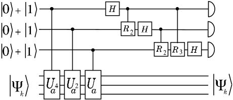
Figure 2: We start with $(\left|\,0\right\rangle+\left|\,1\right\rangle)(\left|\,0\right\rangle+\left|\,1\right\rangle)(\left|\,0\right\rangle+\left|\,1\right\rangle)\left|\,\Psi_{k}\right\rangle$ $=\sum_{x=0}^{7}\left|\,x\right\rangle\left|\,\Psi_{k}\right\rangle$. The controlled multiplications create the state $\sum_{x=0}^{7}\mbox{exp}(2\pi ik/r)\left|\,x\right\rangle\left|\,\Psi_{k}\right\rangle$. The remaining gates create the state $\big{|}\,\widetilde{k/r}\big{\rangle}$ (apart from reversing the order of the qubits) which we then observe. The $H$-gates correspond to Hadamard transforms, and the $R_{j}$-gates correspond to a controlled phase shift of $\mbox{exp}(2\pi i/2^{j})$ on state $\left|\,1\right\rangle$.

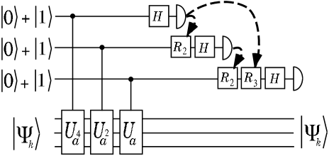
Figure 3: Here we employ a ‘semi-classical’ version of $F_{2^{3}}^{-1}$. We could measure each qubit before it is used as a control, perform the controlled rotations ‘semi-classically’, and the probability of observing each possible output state $\left|\,x_{1}\right\rangle\left|\,x_{2}\right\rangle\left|\,x_{3}\right\rangle$ is the same as in Fig. 2.

Figure 2 shows the relationship between $F_{2^{n}}^{-1}$ and the controlled multiplications by powers of $a$ in the order-finding algorithm. As already pointed out in [GN], the measurements could be performed before the controlled rotations. The quantum controlled rotations could then be replaced with ‘semi-classically’ controlled rotations of the subsequent qubits (that is, the control bit is measured and, if the outcome is $1$, the rotation is done quantumly). This brings us to Fig. 3, where we observe further that all the operations on the first qubit could be performed before we even prepare the second qubit. All the operations could be done sequentially, starting from the first qubit, the results of measuring the previous qubits determining how to prepare the next qubit before measurement. This means we could in fact do all the quantum controlled multiplications with a single control qubit provided we can execute the ‘semi-classical’ controls which allow us to reset a qubit to $\left|\,0\right\rangle+\left|\,1\right\rangle$ and perform a rotation dependent upon the previous measurements (the rotations could in fact be implemented at any time after resetting the qubit and before applying the final Hadamard transform and measuring it; they could also be omitted provided we repeat each step a few extra times and do some additional classical post-processing as done in [Ki]). Alternatively, the control qubits could be a sequence of flying qubits which are measured (or prepared) in a way dependent upon the outcomes of the previous measurements of control qubits.

For the more general hidden subgroup problem in Abelian groups we would have a sequence of applications of $U_{f(\mbox{x}{\mathbf{e_{j}}})}$ controlled by one qubit, which is measured, then reset to a superposition of $\left|\,0\right\rangle$ and $\left|\,1\right\rangle$ plus some rotation that is dependent upon the previous measurements. In summary:

The hidden subgroup $K$ of a finitely generated Abelian group $G$ generated by ${\mathbf{e_{1}}},{\mathbf{e_{2}}},\ldots{\mathbf{e_{k}}}$, corresponding to a function $f$ from $G$ to a finite set $X$, can be found with probability close to $1$ by ‘semi-classical’ methods with only one control bit (or a sequence of flying qubits) and polynomial in $n$ applications of the operators $\left|\,x\right\rangle\left|\,f({\mathbf{y}})\right\rangle\rightarrow\left|\,x\right\rangle\left|\,f({\mathbf{y}}+x{\mathbf{e_{j}}})\right\rangle$ for $j=1,2,\ldots,k$, where $n$ is the index of $K$ in $G$.

Appendix: When $f$ is many-to-1 on $G/K$

The question of what happens when $f$ is many-to-1 on cosets of $K$ was first addressed in [BL]. This is a slight weakening of the promise that $f$ is distinct on each coset. Suppose $f$ can have up to $m$ cosets going to the same output, for some known $m$. That is, $f=h\circ g$ where $g$ is a homomorphism from $G$ to a some group $H$ with kernel $K$, and $h$ is a mapping from $H$ to $X$ that is at most $m$-to-1. If $m$ divides the order of $K$, we clearly have a problem. For example, suppose $K$ is the cyclic group of order $2M$, and $m=2$, but by changing one value of $f$ it would have period $M$. It can easily be shown that $\Omega(\sqrt{M})$ (that is, at least $c\sqrt{M}$ for some positive constant $c$) applications of $f$ are necessary to distinguish such a modified $f$ from the original one with probability greater than $3/4$, and thus no polynomial time algorithm, quantum or classical, could distinguish the two cases. Thus one requirement for there to exist an efficient solution in the worst case is that $m$ is less than the smallest prime factor of $|K|$, the number of elements in $K$.

The problem when $f$ is not 1-to-1 is the following. Running the same quantum algorithm will produce the state

$$\sum_{k=0}^{r-1}\big{|}\,\widetilde{{k/r}}\big{\rangle}\left|\,\Psi_{k}^{\prime}\right\rangle$$

where

$$\left|\,\Psi_{k}^{\prime}\right\rangle=\sum_{t=0}^{r-1}\mbox{exp}(-2\pi ikt/r)\left|\,f(t)\right\rangle.$$

This is the same definition as in (7) except now the $\left|\,f(t)\right\rangle$ are not necessarily distinct. This means the sizes of each of the $\left|\,\Psi_{k}^{\prime}\right\rangle$ are not necessarily the same since both destructive and constructive interference can occur. Also, the $\left|\,\Psi_{k}^{\prime}\right\rangle$ are no longer orthogonal, and thus some constructive interference could occur on the poor estimates of $k/r$. Recall that even the close estimates of $k/r$ will not yield useful results when $k=0$. Any other $k$ will at least reveal a small factor of $r$. So we need to guarantee that the probability of observing a close enough estimate of $k/r$ for some $k\neq 0$ is significant.

By making our estimates precise enough, say by using over $2\log_{2}r+\epsilon/m^{2}$ control qubits, the estimates of $k/r$ will have error less than $1/2r^{2}$ (so that continued fractions will work) with probability at least $1-\epsilon/m^{2}$. Thus assuming $f$ is 1-to-1, the probability of observing a bad output other than $0$ would be at most $\epsilon/m^{2}$, and the probability of observing $0$ would be at most $1/r+\epsilon/m^{2}$. However, since $f$ is at most $m$-to-1, these probabilities could amplify by at most a factor of $m^{2}$ to $\epsilon$ and $m^{2}/r+\epsilon$ respectively. Observing a $0$ means we either got a bad output, or the period of $f$ is $1$. Getting $0$ as a bad output is not very harmful, however getting another bad output is more complicated, since it will give us a false factor of $r$. It will be useful to make $\epsilon$ small, so that it is unlikely our answer is tainted by false factors of $r$. Once we have one factor $r_{1}$ of $r$, we can replace $f(x)$ with $f(r_{1}x)$ (as done in [BL]), which has period $r/r_{1}$ and find a factor of $r/r_{1}$. Once we have a big enough factor $r^{\prime}$ of $r$, we might start observing $0$’s, which tells us that the remaining factor of the original $r$, namely $r/r^{\prime}$, is less than $m^{2}$. Thus we can explicitly test $f(r^{\prime}),f(2r^{\prime}),f(3r^{\prime}),\ldots,$ until we find the period, which will occur after at most $m^{2}$ applications. We thus have an algorithm with running time, in terms of elementary quantum operations and applications of $f$, polynomial in $\log(r)$ and quadratic in $m$.

The trick of reducing the order of the function can be applied to reduce the size of the group and hidden subgroup in the finite Abelian hidden subgroup problem. When $G={\mathbf{Z}}_{p}$, we can efficiently test if $K=G$ or $K=\{1\}$. The above analysis tells us how to deal with the case that $G={\mathbf{Z}}_{p^{l}}$ for $n>1$. A similar technique will reduce $G={\mathbf{Z}}_{p^{l_{1}}}\times\cdots{\mathbf{Z}}_{p^{l_{k}}}$ to a quotient group $\overline{G}$ and we can again proceed inductively until the size of $\overline{G}$ is less than $m^{2}$. We can then exhaustively test $\overline{G}$ for the hidden subgroup $\overline{K}$ in another $O(m^{2})$ steps.

We emphasize that this is a worst-case analysis. If there were a noticeable difference in the behaviour of a 1-to-1 and an $m$-to-1 function $f$, $m>1$, we could decide if a given function $h$ is 1-to-1 or many-to-one (by composing $h$ with a function $f$ whose period or hidden Abelian subgroup we know, and test for this difference in behaviour). Distinguishing 1-to-1 functions from many-to-1 functions seems like a very difficult task in general, and would solve the graph automorphism problem, for example.

References

- [BBCDMSSSW] Barenco, A., Bennett, C.H., Cleve, R, DiVincenzo, D.P., Margolus, N., Shor, P., Sleater, T., Smolin, J., Weinfurter, H.: Phys. Rev. A 52, (1995) 3457.
- [BL] Boneh, D., and Lipton, R.J.: Quantum cryptanalysis of hidden linear functions (Extended abstract). Lecture Notes on Computer Science 963 (1995) 424–437
- [CEMM] Cleve, R., Ekert, E., Macchiavello, C., and Mosca, M.: Quantum Algorithms Revisited, Proc. Roy. Soc. Lond. A, 454, (1998) 339-354.
- [De] Deutsch, D. : Quantum Theory, the Church-Turing principle and the universal quantum computer. Proc. Roy. Soc. Lond. A, 400, (1985) 97-117.
- [EM] Ekert, A., Mosca, M.: (note in preparation, 1998).
- [GN] Griffiths, R.B. and Niu, C.-S.: Semi-classical Fourier Transform for Quantum Computation, Phys. Rev. Lett. 76 (1996) 3228-3231.
- [Gr] Grigoriev, D. Y.: Testing the shift-equivalence of polynomials by deterministic, probabilistic and quantum machines. Theoretical Computer Science, 180 (1997) 217-228.
- [Hø] Høyer, P. : Conjugated Operators in Quantum Algorithms. preprint, (1997).
- [Jo] Jozsa, R.: Quantum Algorithms and the Fourier Transform, Proc. Roy. Soc. Lond. A, 454, (1998) 323-337.
- [Ki] Kitaev, A. Y. : Quantum measurements and the Abelian stabiliser problem. e-print quant-ph/9511026 (1995)
- [LP] Lenstra, H. W. Jr., and Pomerance, C.: A Rigorous Time Bound For Factoring Integers, Journal of the AMS, Volume 5, Number 2, (1992) 483-516.
- [MOV] Menezes, A., van Oorschot, P., Vanstone, S. : Handbook of Applied Cryptography, C.R.C. Press, 1997.
- [Sh] Shor, P. : Algorithms for quantum computation: Discrete logarithms and factoring. Proc. 35th Ann. Symp. on Foundations of Comp. Sci. (1994) 124–134
- [Si] Simon, D.: On the Power of Quantum Computation. Proc. 35th Ann. Symp. on Foundations of Comp. Sci. (1994) 116–123
- [THLMK] Turchette, Q.A., Hood C.J., Lange W., Mabuchi H., and Kimble H.J.: Measurement of conditional phase shifts for quantum logic. Phys. Rev. Lett. , 76, 3108 (1996).