The Schrödinger particle in an oscillating spherical cavity

Abstract

We study a Schrödinger particle in an infinite spherical well with an oscillating wall. Parametric resonances emerge when the oscillation frequency is equal to the energy difference between two eigenstates of the static cavity. Whereas an analytic calculation based on a two-level system approximation reproduces the numerical results at low driving amplitudes $\epsilon$, we observe a drastic change of behaviour when $\epsilon>0.1$, when new resonance states appear bearing no apparent relation to the eigenstates of the static system.

We study in this article the behaviour of a Schrödinger particle confined in a spherical cavity with an oscillating boundary that constitutes a particular kind of time-dependent perturbation. Our study provides a conceptually simple “laboratory” in which the subtle and nontrivial aspects of the resonant coupling between the oscillating wall and a particle trapped inside the cavity can be investigated. Our original motivation in this work comes from our attempt to construct a dynamical bag model of hadrons [1]; however, our results may bear implications on the physics of a wide range of systems such as cavity QED [2] and perhaps even sonoluminescence [3].

The system of a one-dimensional vibrating perfect cavity with quantized electromagnetic fields has been well studied [2]. It was found that the electromagnetic field energy density inside a cavity vibrating at one of its resonance frequencies concentrates into narrow peaks regardless of the detailed trajectories of the oscillating cavity wall [4, 5, 6]. Furthermore, the amplitudes of these energy wave packets grow rapidly in time, producing sharp and intense pulses of photons. The distortion of the vacuum fields arising from the cavity wall motions leads to dynamical modifications of the Casimir effects [7], which represents a fundamentally important and interesting feature of quantum physics. The problem of a quantum particle in a box with moving walls has also been studied with an analytical approach [10], but the possibility of resonances was not discussed, which is the main interest in this work.

If the oscillation amplitude $\epsilon R_{0}$ is small compared to the original cavity radius $R_{0}$, perturbation theory can be used to calculate the transition amplitudes between two states of the unperturbed system. This corresponds to what is usually observed in experiments. However the non-perturbative solutions of the complete time-dependent Hamiltonian ($H=H_{0}+H_{1}(t)$), where $H_{0}$ is the time-independent part of the Hamiltonian, can in principle be remarkably different from the perturbative ones and can give rise to non-trivial features.

We consider, as a first step, an infinite spherical well with oscillating walls:

$$V(r)=\left\{\begin{array}[]{ll}0&\mbox{if $r<R(t)$}\\ \infty&\mbox{if $r\geq R(t)$}\end{array}\right.,$$ (1)

where $R(t)=R_{0}(1+\epsilon\sin{\nu t})\equiv R_{0}/\alpha(t)$. Transforming to a fixed spatial domain via $\vec{y}\equiv\alpha(t)\vec{r}$, $y\equiv|\vec{y}|<R_{0}$, and renormalizing the wavefunction $\phi({\vec{y}},t)\equiv\alpha^{-3/2}(t)\psi({\vec{r}},t)$ in order to preserve unitarity, we have

$$i\hbar{\partial\phi\over\partial t}=H_{0}\phi+H_{1}(t)\phi\ \ ,$$ (2)

where

$$H_{1}(t)\equiv\left(\alpha^{2}(t)-1\right)H_{0}-{\dot{R}(t)\over R(t)}\left(\vec{y}\cdot\vec{p}-i{3\over 2}\hbar\right)\ \$$ (3)

can be considered a small time-dependent perturbation if $\epsilon$ and $\nu$ are small enough.

Since $H_{1}(t)$ commutes with $L^{2}$ and $\vec{L}$, we can look for solutions that are eigenstates of the angular momentum. This allows us to separate the angular dependence from the radial one in Eq. 2 to obtain:

$$\begin{array}[]{ll}{\partial\over\partial t}\phi(y)&=i{\hbar\over 2m}\alpha^{2}(t)\left[{\partial^{2}\over\partial y^{2}}+{2\over y}{\partial\over\partial y}-{l(l+1)\over y^{2}}\right]\phi(y)\\ &+{\dot{R}(t)\over R(t)}\left(y{\partial\over\partial y}+{3\over 2}\right)\phi(y)\ \ .\end{array}$$ (4)

Using first-order perturbation theory, one can easily calculate the coefficients of the solution’s expansion in terms of the unperturbed eigenstates. If the initial state is chosen to be $|i>=|n\!=\!k,l\!=\!0>$ ($\phi_{n,0}=\sqrt{2}n\pi j_{0}(n\pi y)$), we have

$$\begin{array}[]{l}c^{0}_{n}(t)=\delta_{nk}\\ c^{1}_{n}(t)={i\over\hbar}\delta_{nk}E_{k}\int^{t}_{0}dt^{\prime}\left(1-\alpha^{2}(t^{\prime})\right)-\\ (-1)^{n-k}{2nk\over n^{2}-k^{2}}(1-\delta_{nk})\int^{t}_{0}dt^{\prime}e^{{i\over\hbar}(E_{n}-E_{k})t^{\prime}}{\dot{R}(t^{\prime})\over R(t^{\prime})}\ \ .\end{array}$$ (5)

The term due to $i\hbar{\dot{R}(t)\over R(t)}{3\over 2}$ is exactly canceled out by the diagonal contribution of $-{\dot{R}(t)\over R(t)}\vec{y}\cdot\vec{p}$. The last integral is analytically solvable for $\nu=\omega_{nk}=(E_{n}-E_{k})/\hbar$ and yields

$$\begin{array}[]{l}\int^{t}_{0}dt^{\prime}e^{i\omega_{nk}t^{\prime}}{\dot{R}(t^{\prime})\over R(t^{\prime})}={\omega_{nk}t\over\epsilon}+\cos\omega_{nk}t-1\\ -2{\sqrt{1-\epsilon^{2}}\over\epsilon}\left[\arctan\left({\epsilon+\tan\left({\omega_{nk}t\over 2}\right)\over\sqrt{1-\epsilon^{2}}}\right)-\arctan\left({\epsilon\over\sqrt{1-\epsilon^{2}}}\right)\right]\\ +i\left[\sin\omega_{nk}t-{1\over\epsilon}\ln(1+\epsilon\sin\omega_{nk}t)\right]\ \ .\end{array}$$ (6)

The secular term $\omega_{nk}t/\epsilon$ in Eq. 6 is a typical sign of a resonance. Notice that the secular term does not multiply a periodic function and the amplitude $\epsilon$ that we suppose to be small is at the denominator. We can easily check that this is not a problem if we make a Taylor expansion of $\arctan\left[\left(\epsilon+\tan\left({\omega_{nk}t/2}\right)\right)/\sqrt{1-\epsilon^{2}}\right]$ in powers of $\epsilon$ near $\epsilon=0$, since the zeroth-order term exactly cancels the secular term. However the increase of $c^{1}_{n}(t)$ in time remains.

We can now calculate the expectation value of any observable as a function of time. We define the following dimensionless quantities:

$$\begin{array}[]{l}\tilde{E}\equiv mR_{0}^{2}E/\hbar^{2}\ ,\\ \tilde{\nu}\equiv mR_{0}^{2}\nu/\hbar\ .\end{array}$$ (7)

The perturbative results are in excellent agreement with the numerical ones when the cavity is oscillating out of the resonances. For example, at $\tilde{\nu}\!=\!7,\ \epsilon=0.01$ the fluctuations of the energy (Fig. 1) correspond almost exactly to those of ${1/R^{2}(t)}$, as one can expect from a quasistatic approximation, even though our system is not quasistatic. Even at high frequencies such as at $\tilde{\nu}\!=\!90,\ \epsilon=0.01$, the first-order perturbative results are still acceptable (Fig. 2a). Notice that in this case the energy is shifted up slightly and its fluctuations in time are smaller. This is due to the fact that the system is no longer able to follow the fast oscillations of the walls, and consequently the fluctuations as well as the value of the r.m.s. radius $R_{s}\equiv<(y/R_{o})^{2}>^{1/2}$ are suppressed slightly (see Fig. 2b).

At resonances, the perturbative approach breaks down and gives only an indication that a resonance exists. In order to study these resonances we solved the Schrödinger equation numerically, using a unitary numerical algorithm [8]. For $\tilde{\nu}=\tilde{E}_{2}-\tilde{E}_{1}$, we calculated the expectational values of the energy $U\equiv<\tilde{E}>$ and $R_{s}$, choosing $|n=1,l>$ as the initial state. In Fig. 3 we plotted the results for $l\!=\!0$ and $l\!=\!1$ ($l\!=\!0\,,\,\tilde{E}_{2}-\tilde{E}_{1}\!=\!14.8044\,;\,l\!=\!1\,,\,\tilde{E}_{2}-\tilde{E}_{1}\!=\!19.7444$) and two different values of $\epsilon$. The values for $\tilde{\nu}=7$ are also plotted for comparison. The drastic change of behaviour of the system at the resonant frequency is evident even for very small amplitudes such as $\epsilon=0.001$.

At resonances the maximum expectation value of the energy, $U_{\rm max}$, varies as a function of $\epsilon$ because of the trivial adiabatic factor $\alpha^{2}(t)$ and, more importantly, non-trivial excitation processes. In Fig. 4 we show ${\rm max}[\alpha^{-2}(t)U]$ vs. $\epsilon$. For very small $\epsilon$ ($\epsilon<0.002$), the perturbation is not strong enough and the probability of exciting the second eigenstate never reaches $1$. The expectation value of the energy saturates (and equals $\tilde{E}_{2}$) for $0.006<\epsilon<0.1$. In this regime, the frequency dependence of the energy maxima is well fitted by a Breit–Wigner function: $U_{\rm max}=\tilde{E}_{1}+C/[(\tilde{\nu}-\tilde{\nu}_{0})^{2}+\Gamma^{2}/4]$, and the width $\Gamma$ increases linearly with $\epsilon$ up to $\epsilon\approx 0.1$. For $\epsilon>0.1$, even higher states are excited.

Projecting the numerical solution on the eigenstates of the static system we found the expected result that for $\epsilon<0.1$, the resonant dynamics is dominated by the lowest two eigenfunctions. This fact allows us to study the resonating system as a two-level system. In this case the differential equations for the coefficients reduce to:

$$\dot{c}_{1}=-{i\over\hbar}\left[V_{11}(t)c_{1}+V_{12}(t)e^{-i\omega_{21}t}c_{2}\right]\ ,$$ (8)

$$\dot{c}_{2}=-{i\over\hbar}\left[V_{21}(t)e^{i\omega_{21}t}c_{1}+V_{22}(t)c_{2}\right]\;,$$ (9)

where $V_{ij}(t)\equiv<i|H_{1}(t)|j>$. Using the fact that $c_{i}(t)$ changes little in a period $T={2\pi}/\omega_{21}$, we can average Eq. 8 and Eq. 9 over a period to cast them into two coupled first-order ODE’s with constant coefficients [9]:

$$\dot{c}_{i}=\sum_{j}W_{ij}c_{j}\ \ .$$ (10)

Neglecting higher order terms in $\epsilon$, we have

$$W_{11}=W_{22}=0\ ,$$ (11)

$$W_{21}=-W_{12}={4\left(1-\sqrt{1-\epsilon^{2}}\right)\over 3\epsilon}\omega_{21}\equiv\Omega\ \ .$$ (12)

The system can then be diagonalized easily, giving $c_{1}(t)=\cos\Omega t$ and $c_{2}(t)=\sin\Omega t$.

When $\epsilon\ll 1$ then $\Omega\simeq 2\omega_{21}\epsilon/3$ and the period of the resonance $\lim_{\epsilon\rightarrow 0}T_{r}={{2\pi}/\Omega}=\infty$. In the other limit when $\epsilon\rightarrow 1$ then $\Omega\rightarrow{4/3}\>\omega_{21}$, but in this case our assumption that $c_{i}(t)$ changes little in a period is no longer true and the averaging method no more valid. In Fig. 5 we plot the expectation value of the energy $U=\alpha^{2}(t)(\tilde{E}_{1}\cos^{2}\Omega t+\tilde{E}_{2}\sin^{2}\Omega t)$ and compare it with the numerical results. For amplitudes $0.005<\epsilon<0.1$ the agreement is excellent.

The matrix $W_{ij}$ can be written as $-i\Omega\sigma_{2}$, where $\sigma_{2}$ is the second Pauli matrix. It follows that the vector formed by the coefficients $c_{1}$ and $c_{2}$ behaves like the spinor of a spin $1/2$ particle in a magnetic field along the $\hat{\jmath}$ axis:

$$i{\partial|\Psi>\over\partial t}=\Omega\sigma_{2}|\Psi>\ \ .$$ (13)

Therefore, if the initial state of the particle inside the oscillating cavity is one of the two eigenstates involved in the resonance, which corresponds to an eigenstate of $S_{z}$, the evolution of the system will be a precession of $<\vec{S}>$ around the $\hat{\jmath}$ axis. On the other hand, if the initial state corresponds to an eigenstate of $S_{y}$ we will obtain a stationary solution: $|\Psi(t)>=e^{\mp i\Omega t}|\Psi(0)>$, which translates to

$$\phi_{\pm}(y,t)=\sqrt{\alpha^{3}(t)\over 2}e^{\mp i\Omega t}\left[e^{-i{E_{1}\over\hbar}t}\phi_{1}(y)\pm ie^{-i{E_{2}\over\hbar}t}\phi_{2}(y)\right].$$ (14)

The wavefunction in Eq. 14 is periodical with period $T=2\pi/\omega_{21}$:

$$\begin{array}[]{lll}\phi_{\pm}\left(y,t+T\right)=e^{i\theta}\phi_{\pm}\left(y,t\right)\ \ ,\end{array}$$ (15)

where $\theta\equiv-2\pi[E_{2}/(\hbar\omega_{21})\pm 4(1-\sqrt{1-\epsilon^{2}})/3\epsilon]$.

We calculated numerically the solution choosing as initial function one of the two of Eq. 14 at $t=0$, and in Fig. 5 we show the resulting $U$. Although $\alpha^{2}(t)U(t)$ is not strictly constant its variation is considerably smaller compared to other solutions. It is remarkable that such a highly dynamical system can show a quasi-stationary behaviour.

For $\epsilon>0.1$ the two-level approximation starts to break down. For $\epsilon=0.15$ the third and fourth eigenstates become as important as the first two, and even more states are involved as one increases $\epsilon$ further. The behaviour of the system changes drastically for $\epsilon>0.1$, and we even observe the emergence of several new resonances that seem to have no straightforward explanation in terms of the unperturbed eigenstates. In Fig. 6 we show the maxima of $\alpha^{2}(t)U(t)$ computed numerically for several driving frequencies choosing as initial state $|n=1,l=0>$. The resonance at $\nu=\omega_{21}$ is indicated, and it is much broader and smaller in amplitude compared to the new non-trivial resonances. It is interesting to note that even at these new resonances, the coefficients of the expansion in the static eigenstates are still approximately periodic. It may be possible to understand these new resonances for $\epsilon>1$ by including a few more levels in the two-level approximation. However the complexity of the system in this case warrants further study.

For $\epsilon<0.005$ the two-level approximation fails again; it continues to give the maximum of the expected energy as $\tilde{E}_{2}$, typical of two-level systems, while in the complete system the energy maximum decreases as $\epsilon$ is reduced. Also, the two-level approximation gives a period of the resonance $T_{r}$ greater than that of the complete system.

We emphasize that the resonances we studied here are caused exclusively by the motion of the cavity wall, since the system has no interaction with electromagnetic fields. Another interesting feature of our system is the independence of its dynamics on $R_{0}$ except for the rescaling of the oscillating frequency.

It is also possible to consider a real system, hence with the electromagnetic interaction, in which an “oscillating-cavity” resonance occurs but the Rabi resonances do not. In fact, to observe Rabi resonances we need a cavity with radius $R_{0}$ such that the fundamental frequency of the electromagnetic field $\nu_{0}={{2\pi}c/R_{0}}$ is equal to the difference between two energy levels, $E_{n}-E_{k}\propto\hbar^{2}\pi^{2}/2mR_{0}^{2}$. It is hence not difficult to choose an $R_{0}$ such that the Rabi resonances are not excited. In practice though, maintaining a stable mechanical oscillation with frequencies higher than some MHz is difficult.

For simplicity we have only considered a spherically symmetric cavity with perfect wall. However, we conjecture that the resonances should not be too sensitive on the symmetry of the perturbation and on the detailed shape of the potential as long as the matrix element $V_{12}$ (see Eq. 9) is different from zero. One possibility is to use a microcrystal of conducting material with separations between the levels inside the conduction band of the order of $10^{-11}$ eV ($\sim 100$ kHz). Forcing the crystal to vibrate at one of the resonant frequencies should excite many of the Fermi level electrons, which decay by emitting radiowaves. A second way could be to use a system with several, almost equispaced, energy levels. At a resonant frequency the particle, an electron or a trapped atom for example, absorbs energy from the driving oscillation to jump from one level to the next one and so on, as long as the resonance condition $\tilde{\nu}\simeq\tilde{E}_{n+1}-\tilde{E}_{n}$ is satisfied. In this way the frequency of the emitted quanta can be higher than the oscillation frequency, making them distinguishable from the electromagnetic noise due to dipole radiation at the driving frequency.

In a further study we will consider a system with many equispaced energy levels and analyze the increase in energy with time. Ideally from such a system one can get quanta of frequency much higher than the driving frequency, and this is a major difference compared to the cavity QED situation, where at resonances typically a great increase in the number of photons with the same frequency as the driving force is expected.

We thank Dr. C. K. Law for his suggestion of the two-level approximation. This work is partially supported by the Hong Kong Research Grants Council grant CUHK 312/96P and a Chinese University Direct Grant (Project ID: 2060093).

FIG. 1.: Expectation value of the energy $U$ vs. time (scaled by the oscillation period) for $\tilde{\nu}=7$ and $\epsilon=0.01$. The initial state is chosen to be $|n=1,l=0>$.

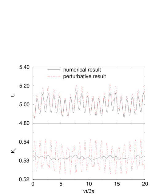
FIG. 2.: (a) Comparison of energy calculated with the perturbative and numerical methods at a high oscillation frequency ($\tilde{\nu}=90,\;\epsilon=0.01$); (b) r.m.s. radius $<(y/R_{0})^{2}>^{1/2}$ for high ($\tilde{\nu}=90$, solid line) and low ($\tilde{\nu}=7$, dashed line) frequencies, both with $\epsilon=0.01$.

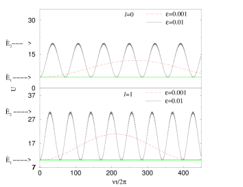
FIG. 3.: Same as Fig. 1, but for (a) $l=0$, $\tilde{\nu}=14.8044$ and (b) $l=1$, $\tilde{\nu}=19.7444$ with $\epsilon=0.001$ (dashed lines) and $\epsilon=0.01$ (solid lines). The arrows indicate the two levels $\tilde{E}_{1}$ and $\tilde{E}_{2}$. For comparison we also plotted the dependence for $\tilde{\nu}=7$, which show up as flat lines near $\tilde{E}_{1}$.

FIG. 4.: Maximum expectation value of the energy $U_{\rm max}$ scaled by the “trivial factor” $\alpha^{2}(t)=(R_{0}/R(t))^{2}$ vs. driving amplitude $\epsilon$ for $\tilde{\nu}=\tilde{E}_{2}-\tilde{E}_{1}$.

FIG. 5.: Same as Fig. 1, but calculated with the two-level approximation (solid line), for $l\!=\!0$, $\epsilon\!=\!0.02$, $\tilde{\nu}=\tilde{E}_{2}-\tilde{E}_{1}=14.8044$. The numerical results are also shown as diamonds. The dotted line shows the numerical result for the special case when $|i>=1/\sqrt{2}(|1>+i|2>)$

FIG. 6.: Maximum expectation value of the energy $U_{\rm max}$ scaled by the “trivial factor” $\alpha^{2}(t)=(R_{0}/R(t))^{2}$ vs. the driving frequency for $l=0$, $\epsilon=0.1$ (solid line), 0.15 (squared line), and 0.2 (dashed line). Several nontrivial resonances appear.

REFERENCES

- [1] P. Hasenfratz and J. Kuti, Phys. Rep. 40, 75 (1978).
- [2] G. T. Moore, J. Math. Phys. 11, 2679 (1970); P. W. Milonni, The Quantum Vacuum (Academic Press, New York, 1993); N. D. Birrell and P. C. W. Davies, Quantum Fields in Curved Space (Cambridge University Press, Cambridge, 1982).
- [3] B. P. Barber et al., Phys. Rep. 281, 65 (1997), and references therein.
- [4] C. K. Law, Phys. Rev. Lett. 73, 1931 (1994).
- [5] C. K. Cole and W. C. Schieve, Phys. Rev. A 52, 4405 (1995).
- [6] Y. Wu, K. W. Chan, M. -C. Chu and P. T. Leung, Phys. Rev. A 59, 1662 (1999).
- [7] M. T. Jaekel and S. Reynaud, J. Phys. I (France) 2, 149 (1992); V. V. Dodonov, A. B. Klimov and D. E. Nikonov, J. Math. Phys. 34, 2742 (1993); C. K. Law, Phys. Rev. A 49, 433 (1994).
- [8] A. Goldberg, H. M. Schey, J. L. Schwartz, American Journal of Physics, Vol. 35, pp. 177–186 (1967).
- [9] V. V. Dodonov, Phys. Lett. A 213, 219 (1996)
- [10] V. V. Dodonov, A. B. Klimov and D. E. Nikonov, J. Math. Phys. 34, 3391 (1993); A. Munier, J. R. Burgan, M. Feix, E. Fijalkow, J. Math. Phys. 22, 1219 (1981).