Experimental Proposal for Achieving Superadditive Communication Capacities
with a Binary Quantum Alphabet

Abstract

We demonstrate superadditivity in the communication capacity of a binary alphabet consisting of two nonorthogonal quantum states. For this scheme, collective decoding is performed two transmissions at a time. This improves upon the previous schemes of Sasaki et al. [Phys. Rev. A 58, 146 (1998)] where superadditivity was not achieved until a decoding of three or more transmissions at a time. This places superadditivity within the regime of a near-term laboratory demonstration. We propose an experimental test based upon an alphabet of low photon-number coherent states where the signal decoding is done with atomic state measurements on a single atom in a high-finesse optical cavity.

PACS number(s): 03.67.-a, 03.67.Dd, 03.67.Lx, 03.67.Hk, 03.65.Bz, 32.80.-t, 33.55.Ad, 42.65.Pc

I Introduction

This paper is about achieving the maximal information transfer rate possible when information is encoded into quantum systems via the preparation of one or another of two nonorthogonal states. This might at first seem like a questionable thing to consider: for transmissions through a noiseless medium, the maximal transfer rate (or capacity) of 1 bit/transmission is clearly achieved only with orthogonal alphabets. This is because nonorthogonal preparations cannot be identified with complete reliability. However, there are instances in which it is neither practical nor desirable to use such an alphabet. The most obvious example is when a simple laser transmitter is located a great distance from the receiver. The receiver’s field will take on the character of a very attenuated optical coherent state. Because the states become less orthogonal as the power is attenuated, one is confronted with precisely the issue considered here. In this case, one is typically stuck with trying to extract information from quantum states that are not only nonorthogonal, but almost completely overlapping.

The practical method in many situations for compensating for very weak signals is to invest in elaborate receiving stations. For instance, in microwave communication very large-dish antennas are the obvious route. Recently, however, a new quantum mechanical effect has been discovered for the decoding of nonorthogonal signals on separate quantum systems. Traditional signal processing methods have only considered fixed decoding measurements performed on the separate transmissions (see for example Ref. [1]): i.e., taking into account the intrinsic noise generated by the quantum measurement [2], one is left with a basic problem of classical information theory—coding for a discrete memoryless channel [3]. Quantum mechanics, however, allows for more possibilities than this [4]. If one is capable of doing collective measurements on blocks of transmitted signals, it is possible to achieve a greater capacity than one might have otherwise thought [5]—this is referred to as the superadditivity of quantum channel capacities. This is an effect that does not exist classically [3, Lemma 8.9.2]. The physics behind the effect relies on a kind of nonlocality dual to the famous one exhibited by entangled quantum systems through Bell inequality violations [6, 7, 8].

More precisely, a communication rate $R$ is said to be achievable if in $k$ transmissions there is a way of writing $2^{Rk}$ messages with the nonorthogonal alphabet so that the probability of a decoding error goes to zero as $k\rightarrow\infty$. The number $R$ signifies the number of bits per transmission that can be conveyed reliably from the transmitter to the receiver in the asymptotic limit. Clearly the rates that can be achieved will depend on the class of codings used for the messages and the class of quantum measurements allowed at the receiver. The capacity $C_{n}$ is defined to be the supremum of all achievable rates, where $n$ is the number of transmissions to be saved up before performing a measurement. The meaning of superadditivity is simply that $C_{n}>C_{1}$, where the inequality is strict.

Generally it is a difficult problem to calculate $C_{n}$ even with a quantum version of Shannon’s noisy channel coding theorem available [5]. And it is a much more difficult task still to find codes that approach $C_{n}$. This is because the coding theorems generally give no information on how to construct codes that approach a given capacity. It turns out however that the number $C_{1}$ is rather easily calculable and, because of a recent very powerful theorem on quantum channel capacities [9, 10, 11], so is the asymptotic case $C_{\infty}$ [8]. The most striking thing about these two quantities is that even though both $C_{1}\rightarrow 0$ and $C_{\infty}\rightarrow 0$ as the overlap between the states goes to unity, the ratio $C_{\infty}/C_{1}$ nevertheless diverges. This means that grossly collective measurements can, in principle at least, produce an arbitrarily large improvement in the channel capacity of very weak signals—a very desirable state of affairs and one of some serious practical import.

The problem from the practical side of the matter is that before one will be able to decode very large blocks, one must first be able to tackle the case of small blocks, preferably of just size two or three. There has already been substantial progress in this direction by Sasaki et al., in a series of papers [12, 13, 14]. They explicitly demonstrate a code that uses collective decoding three transmissions at a time to achieve a communication rate $R_{3}$ greater than $C_{1}$. Nevertheless, it would be nice to demonstrate superadditivity with an even simpler scheme, namely two-shot collective measurements. Also the ratio $R_{3}/C_{1}\rightarrow 1$ as the angle $\gamma$ between the two states goes to zero for their given coding scheme. Thus just where one would be looking for the most help from superadditivity (in the very weak signal regime), one loses it for this code.

We improve on the work of Sasaki et al., by showing that in fact $C_{2}>C_{1}$ for angles $\gamma\lesssim 19^{\circ}$, and moreover that this superadditivity is sustained and only strengthened as $\gamma\rightarrow 0$. On the down side, the improvement in capacity is not great—only 2.82 percent—but is definitely there and not so small as to be forever invisible. In this vein, we propose an experimental demonstration that relies on near-term laboratory capabilities for implementation. For our two nonorthogonal quantum states, we use low photon-number coherent states $|\alpha\rangle$ and $|-\alpha\rangle$ with the separate signals carried on different circular polarizations. The two-shot signal decoding is performed with atomic state measurements on a single Cesium atom in a high-finesse optical cavity via the technique of quantum jumps in fluorescence similar to those demonstrated on ions in Refs. [15, 16, 17].

The remainder of the paper is organized as follows. In the next Section, we demonstrate explicitly that $C_{2}>C_{1}$ for an alphabet of two nonorthogonal states and compare that to the rate $R_{3}$ found in Refs. [12, 13, 14]. In Section III, we specialize this calculation to the coherent states mentioned above and approximate the decoding scheme of Section II with a related scheme that is first order in the small parameter $\alpha$. Finally, in Section IV, we delineate the details of our experimental proposal.

II Deriving Superadditivity for Two-Shot Collective Measurements

Following the discussion in the Introduction, we will take as an alphabet for all communication schemes a fixed set of two nonorthogonal quantum states $|\psi_{0}\rangle$ and $|\psi_{1}\rangle$ characterized by the single parameter $\gamma$:

$$\langle\psi_{0}|\psi_{1}\rangle=\cos\gamma\;.$$ (1)

We would like to know what communication rates $R_{n}$ can be achieved with this alphabet when decoding measurements are performed $n$ transmissions at a time.

This in general is a very difficult problem, especially if one is also confronted with the issue of explicitly demonstrating codes for achieving those rates. However, if one can be contented in knowing the number $C_{n}$ itself and the quantum measurements required to achieve that (i.e., without knowing the coding scheme explicitly), then a great simplification arises because of a quantum extension to the Shannon noisy coding theorem [3] due to Holevo [5].

We shall state the result of this theorem presently. Let the variable $x$ denote the binary strings of length $n$ that index the set of all messages $|\Psi_{x}\rangle=|\psi_{x_{1}}\rangle|\psi_{x_{2}}\rangle\cdots|\psi_{x_{n}}\rangle$, let the function $p(x)$ denote a probability distribution over those messages, and let

$$\rho=\sum_{x}p(x)|\Psi_{x}\rangle\langle\Psi_{x}|$$ (2)

denote the resultant density operator of that distribution. We shall use the notation $E$ to denote a generalized quantum measurement or positive operator-valued measure (POVM) [18] on the message Hilbert space ${\cal H}_{n}$, i.e., $E=(E_{k})$ is an infinite sequence of operators on ${\cal H}_{n}$ with only a finite number of $E_{k}\neq 0$ such that $\langle\psi|E_{k}|\psi\rangle\geq 0$ for all $k$ and $|\psi\rangle$, and the $E_{k}$’s form a decomposition of the identity operator on ${\cal H}_{n}$. In order to find $C_{n}$, it is enough to perform the following maximization:

$$C_{n}=\frac{1}{n}\max_{p(x)}\,\max_{\rm E}\left[H_{\rm\scriptscriptstyle E}(\rho)-\sum_{x}p(x)H_{\rm\scriptscriptstyle E}(|\Psi_{x}\rangle)\right]\;,$$ (3)

where

$$H_{\rm\scriptscriptstyle E}(\rho)=-\sum_{k}({\rm tr}\rho E_{k})\log({\rm tr}\rho E_{k})$$ (4)

and

$$H_{\rm\scriptscriptstyle E}(|\Psi_{x}\rangle)=-\sum_{k}\langle\Psi_{x}|E_{k}|\Psi_{x}\rangle\log\langle\Psi_{x}|E_{k}|\Psi_{x}\rangle$$ (5)

are the Shannon informations for the various probability distributions generated by the measurement $E$. (In these expressions we have used the base-two logarithm so that information is measured in bits.) For any rate $R_{n}=C_{n}-\epsilon$, $\epsilon>0$, there exists a code that will achieve that rate. Moreover, if $E$ is fixed and only the maximization over $p(x)$ is performed in Eq. (3), then the resulting expression will define the capacity that can be reached with the given measurement.

There are two limiting cases where the calculation of $C_{n}$ becomes tractable, $n=1$ and $n=\infty$. In the first case, one can use Refs. [19, 20, 8] to find rather easily that

$$C_{1}(\gamma)= \frac{1}{2}\left[1+\sqrt{1-\cos^{2}\gamma}\,\right]\log\left[1+\sqrt{1-\cos^{2}\gamma}\,\right]$$ (7)

$$+\frac{1}{2}\left[1-\sqrt{1-\cos^{2}\gamma}\,\right]\log\left[1-\sqrt{1-\cos^{2}\gamma}\,\right]\;.$$

For the limit where arbitrarily many collective measurements are made, one can use the powerful theorem of Ref. [9] to find that the channel capacity per bit is given by [8]

$$C_{\infty}(\gamma)= - \frac{1}{2}(1-\cos\gamma)\log\frac{1}{2}(1-\cos\gamma)$$ (8)

$$- \frac{1}{2}(1+\cos\gamma)\log\frac{1}{2}(1+\cos\gamma)\;.$$ (9)

For all cases in between, there is nothing better to be done than an explicit search over all probabilities $p(x)$ and all measurements $E$.

As stated in the Introduction, one can see from Eqs. (7) and (9), that

$$\lim_{\gamma\rightarrow 0}\frac{C_{\infty}(\gamma)}{C_{1}(\gamma)}\;\;\longrightarrow\;\;\infty\;.$$ (10)

So the incentive to use collective measurements in the decoding of these signals is great.

Therefore, let us specialize to the case of collective measurements on two transmissions at a time. In this case, with respect to the decoding observables we have an effective alphabet consisting of the tensor-product states

$$|a\rangle = |\psi_{0}\rangle|\psi_{1}\rangle$$ (11)

$$|b\rangle = |\psi_{1}\rangle|\psi_{0}\rangle$$ (12)

$$|c\rangle = |\psi_{0}\rangle|\psi_{0}\rangle$$ (13)

$$|d\rangle = |\psi_{1}\rangle|\psi_{1}\rangle\;,$$ (14)

with the consequent inner products

$$\langle a|c\rangle=\langle b|c\rangle=\langle a|d\rangle=\langle b|d\rangle=\cos\gamma\;,$$ (15)

and

$$\langle a|b\rangle=\cos^{2}\gamma\;.$$ (16)

It turns out that these states can already exhibit superadditivity even when the collective observables are taken to be simple von Neumann measurements: i.e., by taking $E_{k}=|e_{k}\rangle\langle e_{k}|$ where the $|e_{k}\rangle$ are four orthonormal vectors. Taking $p_{i}$ to be a probability distribution on the effective alphabet states, we must attempt to maximize the rate

FIG. 1.: The ratio $C_{\infty}/C_{1}$ as a function of the angle $\gamma$ in degrees, where $\gamma$ is the angle between the two nonorthogonal states comprising the transmission alphabet.

$$R= H_{\rm\scriptscriptstyle E}(\rho)-p_{a}H_{\rm\scriptscriptstyle E}(|a\rangle)-p_{b}H_{\rm\scriptscriptstyle E}(|b\rangle)-p_{c}H_{\rm\scriptscriptstyle E}(|c\rangle)$$ (18)

$$-p_{d}H_{\rm\scriptscriptstyle E}(|d\rangle)$$

with

$$\rho=p_{a}|a\rangle\langle a|+p_{b}|b\rangle\langle b|+p_{c}|c\rangle\langle c|+p_{d}|d\rangle\langle d|\;,$$ (19)

$$H_{\rm\scriptscriptstyle E}(\rho)=-\sum_{k}\langle e_{k}|\rho|e_{k}\rangle\log\langle e_{k}|\rho|e_{k}\rangle\;,$$ (20)

and

$$H_{\rm\scriptscriptstyle E}(|a\rangle)=-\sum_{k}|\langle e_{k}|a\rangle|^{2}\log|\langle e_{k}|a\rangle|^{2}$$ (21)

and likewise for $|b\rangle$, $|c\rangle$, and $|d\rangle$. The rate $R_{2}$ we will be interested in is then

$$R_{2}=\frac{1}{2}\max_{p_{i}}\,\max_{|e_{k}\rangle}R\;.$$ (22)

We have thoroughly studied $R_{2}$ numerically with a steepest descent and simulated annealing technique. As one might guess, the optimal solution to Eq. (22)—for sufficiently small angles ($\gamma\lesssim 19^{\circ}$)—appears to obey the following symmetries

$$p_{d} \rightarrow 0,$$ (23)

$$p_{a} = p_{b}\equiv p,$$ (24)

$$p_{c} \equiv 1-2p.$$ (25)

Therefore we make the following Ansatz (see Fig. 2)

$$\langle c|e_{3}\rangle = \cos\eta$$ (26)

$$\langle a|e_{1}\rangle = \langle b|e_{2}\rangle$$ (27)

$$\langle a|e_{3}\rangle = \langle b|e_{3}\rangle$$ (28)

$$\langle c|e_{1}\rangle = \langle c|e_{2}\rangle$$ (29)

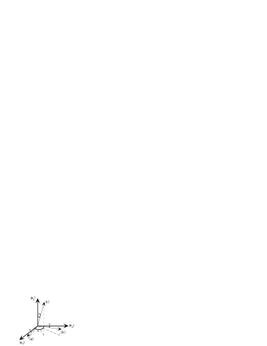
FIG. 2.: The effective alphabet for our implementation represented in an orthogonal measurement basis. The projections are in the $|e_{1}\rangle$,$|e_{2}\rangle$ plane.

FIG. 3.: The solid line represents the ratio $R_{2}/C_{1}$ as a function of $\gamma$. The dashed line represents the ratio obtained using the experimentally feasible but nonoptimal basis discussed in Section III. The dotted line represents $R_{3}/C_{1}$ obtained by Sasaki et al. in Refs. [12, 13, 14].

Taking these symmetries as a more analytic starting point, we can expand the measurement basis as a function of $\eta$, $\gamma$, and the alphabet states (see Fig. 2):

$$|e_{1}\rangle= \frac{\cos\eta+1}{2\sin\gamma}|a\rangle+\frac{\cos\eta-1}{2\sin\gamma}|b\rangle$$ (31)

$$+\frac{\sqrt{2}\sin\eta\sin\gamma-2\cos\eta\cos\gamma}{2\sin\gamma}|c\rangle$$

$$|e_{2}\rangle= \frac{\cos\eta-1}{2\sin\gamma}|a\rangle+\frac{\cos\eta+1}{2\sin\gamma}|b\rangle$$ (33)

$$+\frac{\sqrt{2}\sin\eta\sin\gamma-2\cos\eta\cos\gamma}{2\sin\gamma}|c\rangle$$

$$|e_{3}\rangle= -\frac{\sqrt{2}\sin\eta}{2\sin\gamma}|a\rangle-\frac{\sqrt{2}\sin\eta}{2\sin\gamma}|b\rangle$$ (35)

$$+\frac{\sqrt{2}\sin\eta\cos\gamma+\cos\eta\sin\gamma}{\sin\gamma}|c\rangle$$

Thus the rate can now be expressed as

$$R_{2}(\gamma)=\max_{\eta,p}R(\eta,p,\gamma)$$ (36)

FIG. 4.: The difference in rates $R_{2}-C_{1}$ as a function of the angle $\gamma$.

Even with these strong assumptions and simplifications, $R_{2}(\gamma)$ does not yield a simple analytic expression. We must instead content ourselves with a numerical study as depicted in Figure 3. Note in particular that as $\gamma\rightarrow 0$ the superadditivity does not dwindle away:

$$\lim_{\gamma\rightarrow 0}\frac{R_{2}(\gamma)}{C_{1}(\gamma)}\;\;\longrightarrow\;\;1.02818\;.$$ (37)

This contrasts with the rate $R_{3}$ exhibited by Sasaki et al. [12, 13, 14] for which the ratio $R_{3}/C_{1}$ goes to one within the very weak signal regime.

Note that we use the notation $R_{2}$ rather than $C_{2}$ because our favored quantity can only be asserted as a lower bound to the two-shot capacity. The symmetry assumptions on the probabilities along with the specialization to symmetric von Neumann measurements could turn out to be overly restrictive. However, further numerical investigations seem to indicate that any further improvement is likely to be very small [21]. Also we should emphasize that demonstrating that $R_{2}>C_{1}$ does not give an automatic means for finding a code that comes within $\epsilon$ of this rate: the channel capacity theorem Eq. (3) is only an existence proof of such a code. However, the noise model that our alphabet and measurement leads to—i.e., a simple stochastic transition diagram on three letters—has been extensively studied in classical information-theory literature, and good codes for this problem are likely to exist.

Finally, let us mention one more quantification of the superadditivity due to our nonorthogonal alphabet; this is the simple difference between the two-shot rate and the one-shot rate. We plot $R_{2}-C_{1}$ in Figure 4. It has been suggested in Ref. [8] that the differences $C_{n}-C_{1}$ can help define various notions of when two quantum states are most “quantum” with respect to each other (and hence least “classical”). When one goes to the limit $C_{\infty}-C_{1}$ one finds a well-behaved notion: two states are most quantum with respect to each other when they are $45^{\circ}$ apart. Figure 4 seems to indicate that $R_{2}-C_{1}$ plays no such simple role: at the very least, it means that this difference does a poor job of ferreting out the quantumness of two states in the geometrical sense already supplied by Hilbert space.

III Basis for Experiment

Let us now focus on the case we are most interested in for our experimental proposal: two very low photon-number coherent states $|\alpha\rangle$ and $|-\alpha\rangle$ of a particular field mode. We choose $\alpha$ real so that the mean photon number in that mode is $\alpha^{2}$. For the angles for which we demonstrated superadditivity, i.e., $\gamma\lesssim 19^{\circ}$, this translates to a mean photon number less than 0.03 in each transmission. In this case, we are well warranted in making the approximation

$$|\psi_{0}\rangle = |\alpha\rangle\cong\frac{1}{\sqrt{1+\alpha^{2}}}|0\rangle+\frac{\alpha}{\sqrt{1+\alpha^{2}}}|1\rangle$$ (38)

$$|\psi_{1}\rangle = |-\alpha\rangle\cong\frac{1}{\sqrt{1+\alpha^{2}}}|0\rangle-\frac{\alpha}{\sqrt{1+\alpha^{2}}}|1\rangle\;,$$ (39)

where $|0\rangle$ and $|1\rangle$ denote the zero- and single-photon states of the mode, respectively. Moreover, we have

$$\alpha\cong\sqrt{\frac{1-\cos\gamma}{1+\cos\gamma}}\;.$$ (40)

In order to keep track of the separate transmissions, we encode each transmission in a different mode. For our purposes it is convenient to choose two orthogonal circular polarizations. Expanding the measurement basis in terms of the photon number states, we thus have

$$|e_{1}\rangle= \frac{\sqrt{2}\sin\eta+2\alpha\cos\eta}{2(1+\alpha^{2})}|0\rangle_{+}|0\rangle_{-}$$ (44)

$$+\frac{\alpha\sqrt{2}\sin\eta-\cos\eta+\alpha^{2}\cos\eta-1-\alpha^{2}}{2(1+\alpha^{2})}|0\rangle_{+}|1\rangle_{-}$$

$$+\frac{\alpha\sqrt{2}\sin\eta-\cos\eta+\alpha^{2}\cos\eta+1+\alpha^{2}}{2(1+\alpha^{2})}|1\rangle_{+}|0\rangle_{-}$$

$$+\frac{\alpha^{2}\sqrt{2}\sin\eta-2\alpha\cos\eta}{2(1+\alpha^{2})}|1\rangle_{+}|1\rangle_{-}$$

$$|e_{2}\rangle= \frac{\sqrt{2}\sin\eta+2\alpha\cos\eta}{2(1+\alpha^{2})}|0\rangle_{+}|0\rangle_{-}$$ (49)

$$+\frac{\alpha\sqrt{2}\sin\eta-\cos\eta+\alpha^{2}\cos\eta+1+\alpha^{2}}{2(1+\alpha^{2})}|0\rangle_{+}|1\rangle_{-}$$

$$+\frac{\alpha\sqrt{2}\sin\eta-\cos\eta+\alpha^{2}\cos\eta-1-\alpha^{2}}{2(1+\alpha^{2})}|1\rangle_{+}|0\rangle_{-}$$

$$+\frac{\alpha^{2}\sqrt{2}\sin\eta-2\alpha\cos\eta}{2(1+\alpha^{2})}|1\rangle_{+}|1\rangle_{-}$$

$$|e_{3}\rangle= \frac{\cos\eta-\alpha\sqrt{2}\sin\eta}{(1+\alpha^{2})}|0\rangle_{+}|0\rangle_{-}$$ (54)

$$+\frac{\sqrt{2}\sin\eta(1-\alpha^{2})+2\alpha\cos\eta}{2(1+\alpha^{2})}|0\rangle_{+}|1\rangle_{-}$$

$$+\frac{\sqrt{2}\sin\eta(1-\alpha^{2})+2\alpha\cos\eta}{2(1+\alpha^{2})}|1\rangle_{+}|0\rangle_{-}$$

$$+\frac{\alpha\sqrt{2}\sin\eta+\alpha^{2}\cos\eta}{(1+\alpha^{2})}|1\rangle_{+}|1\rangle_{-}$$

The $+$ and $-$ subscripts in these equations refer to righthand and lefthand circularly polarized light, respectively.

The measurement basis above is, of course, orthonormal. However, after optimizing over $\eta$ as in the previous section, one finds that the coefficient of each $|1\rangle_{+}|1\rangle_{-}$ component turns out to be of order $\alpha$ while the other terms are of order one. Because one is free to choose any measurement basis, we choose to ignore the small $|1\rangle_{+}|1\rangle_{-}$ term for each $|e_{i}\rangle$. This new basis $|\tilde{e}_{i}\rangle$ is close to the optimal basis $|e_{i}\rangle$ but allows the great simplification of not having to worry about how to distinguish $|1\rangle_{+}|1\rangle_{-}$ from $|0\rangle_{+}|1\rangle_{-}$ and $|1\rangle_{+}|0\rangle_{-}$. We may then focus on experiments based on the absorption of at most a single photon.

The final step for defining our measurement scheme is to re-orthogonalize the vectors $|\tilde{e}_{i}\rangle$. A simple convenient technique for this is the one introduced in Ref. [22]. Let

$$M=\sum_{i=1}^{3}|\tilde{e}_{i}\rangle\langle\tilde{e}_{i}|\;.$$ (55)

Then clearly the vectors

$$|e^{\prime}_{i}\rangle=M^{-\frac{1}{2}}|\tilde{e}_{i}\rangle$$ (56)

form an orthonormal set. It is this basis that we will use in the experimental proposal, the main point of interest about it being that it contains no two-photon contributions. Of course, the new basis cannot be optimal for achieving the rate $R_{2}$ already calculated, but for small $\alpha$ it becomes arbitrarily good. In fact, it is already sufficient for demonstrating superadditivity for $\gamma\lesssim 17^{\circ}$ (see Fig. 3).

IV Experimental Proposal

We now turn to the task of realizing the measurement explored in the last section. To carry this out, we need the ability to perform an entangled measurement on two wave packets at a time. We can achieve this collective decoding by mapping the orthonormal measurement basis in Eq. (56) onto a set of orthonormal superpositions of three sublevels of a single atom (see Figure 5).

The basic idea is to first transfer the information from the propagating light fields to photons inside an optical cavity and subsequently map the information from the cavity field to a single atom inside that cavity. This can be accomplished as follows: First, the atom is prepared in a ground state with $|m=0\rangle$ by optical pumping. The presence of a single $\sigma^{+}$ polarized cavity photon is then more than sufficient to induce a Raman transition to the $|m=1\rangle$ state with the help of a $\pi$-polarized laser field (in fact, the advances in cavity QED have increased the

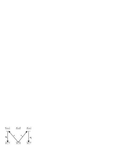
FIG. 5.: Transition diagram for our implementation: a $\pi$-polarized laser field with frequency $\omega_{L}$ is applied to a single atom inside an optical cavity. The laser will induce a Raman transition from the initial state $|m=0\rangle$ to $|m=+1\rangle$ or $|m=-1\rangle$ in the presence of a single $\sigma^{+}$ or $\sigma^{-}$ polarized cavity photon, with frequency $\omega_{C}=\omega_{L}$. No transition is induced in the absence of a cavity photon, as the $m=0\leftrightarrow m^{\prime}=0$ transition is forbidden. Note that $\pi$-polarized modes are not supported by the cavity.

atom-cavity coupling to such a large degree that the saturation photon number for optical transitions is very small[23]; in particular, for the $(6S_{\frac{1}{2}},F=4,m=4)\rightarrow(6P_{\frac{3}{2}},F=5,m=5)$ transition in Cesium it is only $2.3\times 10^{-4}$[24]). Similarly, the presence of a single $\sigma^{-}$ photon will induce the transition to $|m=-1\rangle$, while if no cavity photon is present, the atom will stay in $|m=0\rangle$. Thus, the measurement scheme is based on the mapping

$$|0\rangle_{+}|0\rangle_{-}|m=0\rangle \;\;\longmapsto\;\; |0\rangle_{+}|0\rangle_{-}|m=0\rangle,$$ (57)

$$|0\rangle_{+}|1\rangle_{-}|m=0\rangle \;\;\longmapsto\;\; |0\rangle_{+}|0\rangle_{-}|m=-1\rangle,$$ (58)

$$|1\rangle_{+}|0\rangle_{-}|m=0\rangle \;\;\longmapsto\;\; |0\rangle_{+}|0\rangle_{-}|m=+1\rangle.$$ (59)

This mapping must be executed within the cavity lifetime (a typical lifetime for high-finesse optical cavities is $\kappa^{-1}\sim 0.1\mu$s [25]). Once this mapping has been performed, we no longer rely on cavity fields.

In order to avoid any disturbing effects from the laser field on level $|m=0\rangle$ in the absence of a cavity photon, we require the transition $|m=0\rangle\mapsto|m^{\prime}=0\rangle$ to be forbidden, which is easily accomplished by choosing $\delta F=0$ transitions. For example, one might consider the following transition between hyperfine multiplets in Cesium

$$6S_{\frac{1}{2}},F=3\;\;\longleftrightarrow\;\;6P_{\frac{1}{2}},F=3.$$ (60)

Moreover, the frequency $\omega_{L}$ of the laser field is chosen such that we are on two-photon resonance with the $|m=0\rangle\leftrightarrow|m=\pm 1\rangle$ Raman transitions, but far off resonance with respect to the excited states. Therefore, the latter will not be populated and no further transitions from $|m=1\rangle$ or $|m=-1\rangle$ will occur.

Once the information has thus been transferred from the polarizations to the atom in the cavity, the measurement basis is an orthonormal superposition of the three relevant atomic ground states $|m=-1\rangle$, $|m=0\rangle$, and $|m=1\rangle$. Making a measurement of a superposition of these states is far more difficult than measuring the states themselves. Therefore, we first apply a unitary operation that transforms the basis of Eq. (56) into the physical measurement basis. This operation can be performed by a series of at most 16 appropriately timed Raman pulses [26, 27]. In general, for an $N$ level system, with $N$ even, the unitary evolution can be controlled with a sequence of $N^{2}$ pulses consisting of two distinct perturbations in an alternating sequence[27]. While this scheme is not optimal for $N=3$, it does give an upper bound for the required number of pulses.

Once this transformation of basis has been performed, the only remaining task is to measure the projection onto each of the three possible hyperfine levels of our physical measurement basis. To perform this measurement, a magnetic field is turned on adiabatically, causing a splitting of the energy of these otherwise degenerate hyperfine levels. Next, we use the technique of optical shelving to make a measurement of the levels [15, 16, 17]. With this technique, a Raman pulse is applied to cause a transition from the $|m=1\rangle$ state into a secondary state that can then be driven on resonance to yield a large number of photons. If the atom fluoresces at the driven frequency, the measurement outcome is $m=1$, and the measurement is finished. Otherwise, if no fluorescence is detected, the atom will not be affected by this driving laser and the process is then repeated for the $|m=0\rangle$ and $|m=-1\rangle$ states.

Finally, let us note that atoms can already be held in a cavity for times exceeding $250\mu$s [25], which is nearly sufficient for the measurements and laser manipulations discussed to be performed. In addition, further improvements on trapping atoms in cavities will relax the conditions on timing. The ability to hold single atoms in a cavity for a sufficient period of time will open up a world of possibilities for the field of communication[28, 29, 30].

V Acknowledgements

We thank H. J. Kimble, R. Legere, H. Mabuchi, M. Sasaki, P. W. Shor, and J. A. Smolin for helpful discussions. We thank A. Landahl for a careful reading of the manuscript. This work was supported by the QUIC Institute funded by DARPA via the ARO, by the ONR, and by the NSF. CAF also acknowledges the support of a Lee A. DuBridge Fellowship.

REFERENCES

- [1] C. M. Caves and P. D. Drummond, Rev. Mod. Phys. 66, 481 (1994).
- [2] A. S. Kholevo, Prob. Inf. Transm., 9, 110 (1973).
- [3] T. M. Cover and J. A. Thomas, Elements of Information Theory, (John Wiley & Sons, New York, 1991).
- [4] A. S. Kholevo, Rep. Math. Phys., 12, 273 (1977).
- [5] A. S. Kholevo, Prob. Inf. Transm. 15, 247 (1979).
- [6] A. Peres and W. K. Wootters, Phys. Rev. Lett. 66, 1119 (1991).
- [7] C. H. Bennett, D. P. DiVincenzo, C. A. Fuchs, T. Mor, E. Rains, P. W. Shor, J. A. Smolin, and W. K. Wootters, Phys. Rev. A 59, 1070 (1999).
- [8] C. A. Fuchs, to appear in Quantum Communication, Computing, and Measurement 2, edited by P. Kumar, G. M. D’Ariano, and O. Hirota (Plenum Press, NY, 1998); see also quant-ph/9810032.
- [9] P. Hausladen, R. Jozsa, B. Schumacher, M. Westmoreland, and W. K. Wootters, Phys. Rev. A 54, 1869 (1996).
- [10] A. S. Holevo, IEEE Trans. Inf. Theor. 44, 269 (1998).
- [11] B. Schumacher and M. D. Westmoreland, Phys. Rev. A 56, 131 (1997).
- [12] M. Sasaki, K. Kato, M. Izutsu, and O. Hirota, Phys. Lett. A 236, 1 (1997).
- [13] M. Sasaki, K. Kato, M. Izutsu, and O. Hirota, Phys. Rev. A 58, 146 (1998).
- [14] M. Sasaki, T. Sasaki-Usuda, M. Izutsu, and O. Hirota, Phys. Rev. A 58, 159 (1998).
- [15] W. Nagourney, J. Sandberg, and H. G. Dehmelt, Phys. Rev. Lett. 56, 2797 (1986).
- [16] T. Sauter, W. Neuhauser, R. Blatt, P. E. Toschek, Phys. Rev. Lett. 57, 1696 (1986).
- [17] J. C. Bergquist, R. G. Hulet, W. M. Itano, and D. J. Wineland, Phys. Rev. Lett. 57, 1699 (1986).
- [18] A. Peres, Quantum Theory: Concepts and Methods, (Kluwer Academic, Dordrecht, 1993).
- [19] L. B. Levitin, in Quantum Communications and Measurement, edited by V. P. Belavkin, O. Hirota, and R. L. Hudson, (Plenum Press, NY, 1995).
- [20] C. A. Fuchs and C. M. Caves, Phys. Rev. Lett. 73, 3047 (1994).
- [21] J. A. Smolin, private communication.
- [22] L. P. Hughston, R. Jozsa, and W. K. Wootters, Phys. Lett. A 183, 14 (1993).
- [23] H. J. Kimble, in Cavity Quantum Electrodynamics, edited by P. Berman (Academic Press, San Diego, 1994).
- [24] C. J. Hood, M. S. Chapman, T. W. Lynn, and H. J. Kimble, Phys. Rev. Lett. 80, 4157 (1998).
- [25] H. Mabuchi, J. Ye, H. J. Kimble, Appl. Phys. B, in press (1999); see also quant-ph/9805076.
- [26] C. K. Law and J. H. Eberly, Opt. Expr. 2, 368 (1998).
- [27] G. Harel, V. M. Akulin, Phys. Rev. Lett. 82, 1 (1999).
- [28] J. I. Cirac, P. Zoller, H. J. Kimble, and H. Mabuchi, Phys. Rev. Lett. 78, 3221 (1997).
- [29] S. J. van Enk, J. I. Cirac, and P. Zoller, Science 279, 205 (1998).
- [30] S. J. van Enk, J. I. Cirac, and P. Zoller, Phys. Rev. Lett. 78, 4293 (1997).