BA-TH/316-99

WU-HEP-99-1

Reflection and Transmission in a Neutron-Spin Test of the Quantum Zeno Effect

Ken Machida,⁽¹⁾ Hiromichi Nakazato,⁽¹⁾ Saverio Pascazio,⁽²⁾

Helmut Rauch⁽³⁾ and Sixia Yu⁽⁴⁾

⁽¹⁾Department of Physics, Waseda University Tokyo 169-8555, Japan
⁽²⁾Dipartimento di Fisica, Università di Bari and Istituto Nazionale di Fisica Nucleare, Sezione di Bari, I-70126 Bari, Italy
⁽³⁾Atominstitut der Österreichischen Universitäten
Stadionallee 2, A-1020, Wien, Austria
⁽⁴⁾Institute of Theoretical Physics, Academia Sinica, Beijing 100080, P.R. China

Abstract

The dynamics of a quantum system undergoing frequent “measurements,” leading to the so-called quantum Zeno effect, is examined on the basis of a neutron-spin experiment recently proposed for its demonstration. When the spatial degrees of freedom are duely taken into account, neutron-reflection effects become very important and may lead to an evolution which is totally different from the ideal case.

PACS: 03.80.+r; 03.65.Bz; 03.65.Nk; 04.20.Cv

1 Introduction

A quantum system, prepared in a state that does not belong to an eigenvalue of the total Hamiltonian, starts to evolve quadratically in time [1, 2]. This characteristic behavior leads to the so-called quantum Zeno phenomenon, namely the possibility of slowing down the temporal evolution (eventually hindering transitions to states different from the initial one) [3].

The original proposals that aimed at verifying this effect involved unstable systems and were not amenable to experimental test [4]. However, the remarkable idea [5] to use a two-level system motivated an interesting experimental test [6], revitalizing a debate on the physical meaning of this phenomenon [7, 8]. There seem to be a certain consensus, nowadays, that the quantum Zeno effect (QZE) can be given a dynamical explanation, involving only an explicit Hamiltonian dynamics.

It is worth emphasizing that the discussion of the last few years mostly stemmed from experimental considerations, related to the practical possibility of performing experimental tests. Some examples are the interesting issue of “interaction-free” measurements [9] and the neutron-spin tests of the QZE [8, 10]. In practical cases, one cannot neglect the presence of losses and imperfections, which obviously conspire against an almost-ideal experimental realization, more so when the total number of “measurements” increases above certain theoretical limits.

The aim of the present paper is to investigate an interesting (and often overlooked) feature of what we might call the quantum Zeno dynamics. We shall see that a series of “measurements” (von Neumann’s projections [11]) does not necessarily hinder the evolution of the quantum system. On the contrary, the system can evolve away from its initial state, provided it remains in the subspace defined by the “measurement” itself. This interesting feature is readily understandable in terms of rigorous theorems [2], but it seems to us that it is worth clarifying it by analyzing interesting physical examples. We shall therefore focus our attention on an experiment involving neutron spin [8] and shall see that in fact this enables us to kill two birds with one stone: not only the state of the neutron undergoing QZE will change, but it will do so in a way that clarifies why reflection effects may play a substantial role in the experiment analyzed.

In the neutron-spin example to be considered, the evolution of the spin state is hindered when a series of spectral decompositions (in Wigner’s sense [12]) is performed on the spin state. No “observation” of the spin states, and therefore no projection à la von Neumann is required, as far as the different branch waves of the wave function cannot interfere after the spectral decomposition. Needless to say, the analysis that follows could be performed in terms of a Hamiltonian dynamics, without making use of projection operators. However, we shall use in this paper the von Neumann technique, which will be found convenient because it sheds light on some remarkable aspects of the Zeno phenomenon and helps to pin down the physical implications of some mathematical hypotheses with relatively less efforts.

The paper is organized as follows. We briefly review, in the next section, the seminal theorem for the short-time dynamics of quantum systems, proved by Misra and Sudarshan [2]. Its application to the neutron-spin case is discussed in Sec. 3. In Secs. 4 and 5, unlike in previous papers [8, 10], we shall incorporate the spatial (1-dimensional, for simplicity) degrees of freedom of the neutron and represent them by an additional quantum number that labels, roughly speaking, the direction of motion of the wave packet. A more realistic analysis is presented in Sec. 6. Finally, Sec. 7 is devoted to a discussion. Some additional aspects of our analysis are clarified in the Appendix.

2 Misra and Sudarshan’s theorem

Consider a quantum system Q, whose states belong to the Hilbert space ${\cal H}$ and whose evolution is described by the unitary operator $U(t)=\exp(-iHt)$, where $H$ is a semi-bounded Hamiltonian. Let $E$ be a projection operator and $E{\cal H}E={\cal H}_{E}$ the subspace spanned by its eigenstates. The initial density matrix $\rho_{0}$ of system Q is taken to belong to ${\cal H}_{E}$. If Q is let to follow its “undisturbed” evolution, under the action of the Hamiltonian $H$ (i.e., no measurements are performed in order to get informations about its quantum state), the final state at time $T$ reads

$$\rho(T)=U(T)\rho_{0}U^{\dagger}(T) 2.1$$ ()

and the probability that the system is still in ${\cal H}_{E}$ at time $T$ is

$$P(T)=\mbox{Tr}\left[U(T)\rho_{0}U^{\dagger}(T)E\right]. 2.2$$ ()

We call this a “survival probability:” it is in general smaller than 1, since the Hamiltonian $H$ induces transitions out of ${\cal H}_{E}$. We shall say that the quantum systems has “survived” if it is found to be in ${\cal H}_{E}$ by means of a suitable measurement process [13].

Assume that we perform a measurement at time $t$, in order to check whether Q has survived. Such a measurement is formally represented by the projection operator $E$. By definition,

$$\rho_{0}=E\rho_{0}E,\qquad\mbox{Tr}[\rho_{0}E]=1. 2.3$$ ()

After the measurement, the state of Q changes into

$$\rho_{0}\rightarrow\rho(t)=EU(t)\rho_{0}U^{\dagger}(t)E/P(t), 2.4$$ ()

where

$$P(t)=\mbox{Tr}\left[U(t)\rho_{0}U^{\dagger}(t)E\right] 2.5$$ ()

is the probability that the system has survived. [There is, of course, a probability $1-P$ that the system has not survived (i.e., it has made a transition outside ${\cal H}_{E}$) and its state has changed into $\rho^{\prime}(t)=(1-E)U(t)\rho_{0}U^{\dagger}(t)(1-E)/(1-P)$. We concentrate henceforth our attention on the measurement outcome ($2.4$)-($2.5$).] The above is the standard Copenhagen interpretation: The measurement is considered to be instantaneous. The “quantum Zeno paradox” [2] is the following. We prepare Q in the initial state $\rho_{0}$ at time 0 and perform a series of $E$-observations at times $t_{k}=kT/N\;(k=1,\cdots,N)$. The state of Q after the above-mentioned $N$ measurements reads

$$\rho^{(N)}(T)=V_{N}(T)\rho_{0}V_{N}^{\dagger}(T),\qquad V_{N}(T)\equiv[EU(T/N)E]^{N} 2.6$$ ()

and the probability to find the system in ${\cal H}_{E}$ (“survival probability”) is given by

$$P^{(N)}(T)=\mbox{Tr}\left[V_{N}(T)\rho_{0}V_{N}^{\dagger}(T)\right]. 2.7$$ ()

Equations ($2.6$)-($2.7$) display the “quantum Zeno effect:” repeated observations in succession modify the dynamics of the quantum system; under general conditions, if $N$ is sufficiently large, all transitions outside ${\cal H}_{E}$ are inhibited.

In order to consider the $N\rightarrow\infty$ limit (“continuous observation”), one needs some mathematical requirements: define

$${\cal V}(T)\equiv\lim_{N\rightarrow\infty}V_{N}(T), 2.8$$ ()

provided the above limit exists in the strong sense. The final state of Q is then

$$\widetilde{\rho}(T)={\cal V}(T)\rho_{0}{\cal V}^{\dagger}(T) 2.9$$ ()

and the probability to find the system in ${\cal H}_{E}$ is

$${\cal P}(T)\equiv\lim_{N\rightarrow\infty}P^{(N)}(T)=\mbox{Tr}\left[{\cal V}(T)\rho_{0}{\cal V}^{\dagger}(T)\right]. 2.10$$ ()

One should carefully notice that nothing is said about the final state $\widetilde{\rho}(T)$, which depends on the characteristics of the model investigated and on the very measurement performed (i.e. on the projection operator $E$, which enters in the definition of $V_{N}$). Misra and Sudarshan assumed, on physical grounds, the strong continuity of ${\cal V}(t)$:

$$\lim_{t\rightarrow 0^{+}}{\cal V}(t)=E 2.11$$ ()

and proved that under general conditions the operators ${\cal V}(T)$ (exist for all real $T$ and) form a semigroup labeled by the time parameter $T$. Moreover, ${\cal V}^{\dagger}(T)={\cal V}(-T)$, so that ${\cal V}^{\dagger}(T){\cal V}(T)=E$. This implies, by ($2.3$), that

$${\cal P}(T)=\mbox{Tr}\left[\rho_{0}{\cal V}^{\dagger}(T){\cal V}(T)\right]=\mbox{Tr}\left[\rho_{0}E\right]=1. 2.12$$ ()

If the particle is “continuously” observed, in order to check whether it has survived inside ${\cal H}_{E}$ , it will never make a transition to ${\cal H}-{\cal H}_{E}$. This is the “quantum Zeno paradox.”

An important remark is now in order: the theorem just summarized does not state that the system remains in its initial state, after the series of very frequent measurements. Rather, the system is left in the subspace ${\cal H}_{E}$, instead of evolving “naturally” in the total Hilbert space ${\cal H}$. This subtle point, implied by Eqs. ($2.9$)-($2.12$), is often not duely stressed in the literature.

Notice also the conceptual gap between Eqs. ($2.7$) and ($2.10$): To perform an experiment with $N$ finite is only a practical problem, from the physical point of view. On the other hand, the $N\rightarrow\infty$ case is physically unattainable, and is rather to be regarded as a mathematical limit (although a very interesting one). In this paper, we shall not be concerned with this problem (thoroughly investigated in [10]) and shall consider the $N\to\infty$ limit for simplicity. This will make the analysis more transparent.

3 Quantum Zeno effect with neutron spin

The example we consider is a neutron spin in a magnetic field [8]. (A photon analog was first outlined by Peres [14].) We shall consider two different experiments: Refer to Figures 1(a) and 1(b). In the case schematized in Figure 1(a),

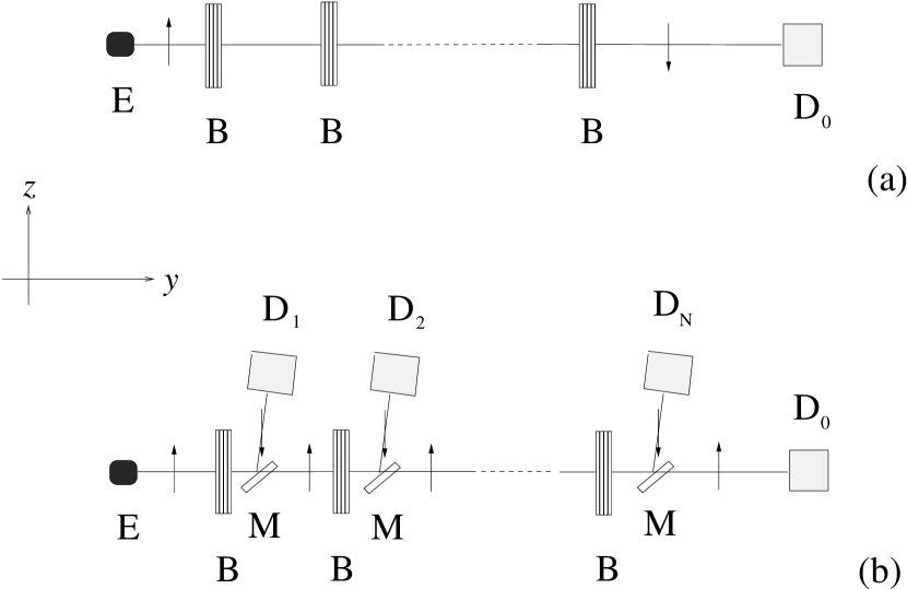
Figure 1: (a) Evolution of the neutron spin under the action of a magnetic field. An emitter sends a spin-up neutron through several regions where a magnetic field $B$ is present. The detector $D_{0}$ detects a spin-down neutron: No Zeno effect occurs. (b) Quantum Zeno effect: the neutron spin is “monitored” at every step, by selecting and detecting the spin-down component. $D_{0}$ detects a spin-up neutron.

the neutron interacts with several identical regions in which there is a static magnetic field $B$, oriented along the $x$-direction. We neglect here any losses and assume that the interaction be given by the Hamiltonian

$$H=\mu B\sigma_{1}, 3.1$$ ()

$\mu$ being the (modulus of the) neutron magnetic moment, and $\sigma_{i}\;(i=1,2,3)$ the Pauli matrices. We denote the spin states of the neutron along the $z$-axis by $|\uparrow\rangle$ and $|\downarrow\rangle$.

Let the initial neutron state be $\rho_{0}=\rho_{\uparrow\uparrow}\equiv|\uparrow\rangle\langle\uparrow|$. The interaction with the magnetic field provokes a rotation of the spin around the $x$-direction. After crossing the whole setup, the final density matrix reads

$$\rho(T)\equiv e^{-iHT}\rho_{0}e^{iHT}=\cos^{2}{\frac{\omega T}{2}}\rho_{\uparrow\uparrow}+\sin^{2}{\frac{\omega T}{2}}\rho_{\downarrow\downarrow}-\frac{i}{2}\sin{\omega T}(\rho_{\uparrow\downarrow}-\rho_{\downarrow\uparrow}), 3.2$$ ()

where $\omega=2\mu B$ and $T$ is the total time spent in the $B$ field. Notice that the free evolution is neglected (and so are reflection effects, wave-packet spreading, etc.). If $T$ is chosen so as to satisfy the “matching” condition $\cos\omega T/2=0$, we obtain

$$\rho(T)=\rho_{\downarrow\downarrow}\qquad\quad\left(T=(2m+1)\frac{\pi}{\omega},\;\;m\in{\bf N}\right), 3.3$$ ()

so that the probability that the neutron spin is down at time $T$ is

$$P_{\downarrow}(T)=1\qquad\quad\left(T=(2m+1)\frac{\pi}{\omega},\;\;m\in{\bf N}\right). 3.4$$ ()

The above two equations correspond to Eqs. ($2.1$) and ($2.2$). In our example, $H$ is such that if the system is initially prepared in the up state, it will evolve to the down state after time $T$. Notice that, within our approximations, the experimental setup described in Figure 1(a) is equivalent to the situation where a magnetic field $B$ is contained in a single region of space.

Let us now modify the experiment just described by inserting at every step a device able to select and detect one component [say the down ($\downarrow$) one] of the neutron spin. This can be accomplished by a magnetic mirror M and a detector D. The former acts as a “decomposer,” by splitting a neutron wave with indefinite spin (a superposed state of up and down spins) into two branch waves each of which is in a definite spin state (up or down) along the $z$-axis. The down state is then forwarded to a detector, as shown in Figure 1(b). The magnetic mirror yields a spectral decomposition [12] with respect to the spin states, and can be compared to the inhomogeneous magnetic field in a typical Stern-Gerlach experiment.

We choose the same initial state for Q as in the previous experiment [Figure 1(a)]. The action of M+D is represented by the operator $E\equiv\rho_{\uparrow\uparrow}$ [remember that we follow the evolution along the horizontal direction, i.e. the direction the spin-up neutron travels, in Figure 1(b)], so that if the process is repeated $N$ times, like in Figure 1(b), we obtain

$$\rho^{(N)}(T)=V_{N}(T)\rho_{0}V_{N}^{\dagger}(T)=\left(\cos^{2}{\frac{\omega t}{2}}\right)^{N}\rho_{\uparrow\uparrow}=\left(\cos^{2}{\frac{\pi}{2N}}\right)^{N}\rho_{\uparrow\uparrow}, 3.5$$ ()

where the “matching” condition for $T=Nt$ [see Eq. ($3.3$)] has been required again. The probability that the neutron spin is up at time $T$, if $N$ observations have been made at time intervals $t\;(Nt=T)$, is

$$P_{\uparrow}^{(N)}(T)=\left(\cos^{2}{\frac{\pi}{2N}}\right)^{N}. 3.6$$ ()

This discloses the occurrence of a QZE: Indeed, $P_{\uparrow}^{(N)}(T)>P_{\uparrow}^{(N-1)}(T)$ for $N\geq 2$, so that the evolution is “slowed down” as $N$ increases. Moreover, in the limit of infinitely many observations

$$\rho^{(N)}(T)\stackrel{{\scriptstyle N\rightarrow\infty}}{{\longrightarrow}}\widetilde{\rho}(T)=\rho_{\uparrow\uparrow} 3.7$$ ()

and

$${\cal P}_{\uparrow}(T)\equiv\lim_{N\rightarrow\infty}P_{\uparrow}^{(N)}(T)=1. 3.8$$ ()

Frequent observations “freeze” the neutron spin in its initial state, by inhibiting ($N\geq 2$) and eventually hindering ($N\rightarrow\infty$) transitions to other states. Notice the difference from Eqs. ($3.3$) and ($3.4$): The situation is completely reversed.

4 The spatial degrees of freedom

In the analysis of the previous section only the spin degrees of freedom were taken into account. No losses were considered, even though their importance was already mentioned in [8, 10]. In spite of such a simplification, the model yields physical insight into the Zeno phenomenon, and has the nice advantage of being solvable.

We shall now consider a more detailed description. The practical realizability of this experiment has already been discussed, with particular attention to the $N\rightarrow\infty$ limit and various possible losses [10]. One source of losses is the occurrence of reflections at the boundaries of the interaction region and/or at the spectral decomposition step. A careful estimate of such effects would require a dynamical analysis of the motion of the neutron wave packet as it crosses the whole interaction region (magnetic-field regions followed by field-free regions containing each a magnetic mirror M that performs the “measurement”). However, it is not an easy task to include the spatial degrees of freedom of the neutron in the analysis; instead, we shall adopt a simplified description of the system, which preserves most of the essential features and for which an explicit solution can still be obtained. It turns out that the inclusion of the spatial degrees of freedom in the evolution of the spin state can result in completely different situations from the ideal case, which in turn clarifies the importance of losses in actual experiments and, at the same time, sheds new light on the Zeno phenomenon itself.

Let us now try to incorporate the other degrees of freedom of the neutron state in our description. Let our state space be the 4-dimensional Hilbert space ${\cal H}_{p}\otimes{\cal H}_{s}$, where ${\cal H}_{p}=\{|R\rangle,|L\rangle\}$ and ${\cal H}_{s}=\{|\uparrow\rangle,|\downarrow\rangle\}$ are 2-dimensional Hilbert spaces, with $R(L)$ representing a particle traveling towards the right (left) direction along the $y$-axis, and $\uparrow(\downarrow)$ representing spin up (down) along the $z$-axis. We shall set, in the respective Hilbert spaces,

$$|R\rangle=\left({1\atop 0}\right),\quad|L\rangle=\left({0\atop 1}\right);\quad|\uparrow\rangle=\left({1\atop 0}\right),\quad|\downarrow\rangle=\left({0\atop 1}\right), 4.1$$ ()

so that, for example, the state $|R\downarrow\rangle$ represents a spin-down particle traveling towards the right direction ($+y$). Also, for the sake of simplicity, we shall work with vectors, rather than density matrices (the extension is straightforward).

In this extended Hilbert space the first Pauli matrix $\sigma_{1}$ acts only on ${\cal H}_{s}$ as a spin flipper, $\sigma_{1}|\uparrow\rangle=|\downarrow\rangle$ and $\sigma_{1}|\downarrow\rangle=|\uparrow\rangle$, while another first Pauli matrix $\tau_{1}$ acts only on ${\cal H}_{p}$ as a direction-reversal operator, $\tau_{1}|R\rangle=|L\rangle$ and $\tau_{1}|L\rangle=|R\rangle$. To investigate the effects of reflection we assume that the interaction be described by the Hamiltonian

$$H=g(1+\alpha\tau_{1})(1+\beta\sigma_{1}), 4.2$$ ()

where $g,\alpha$ and $\beta$ are real constants. By varying these parameters and the total interaction time $T$, the above Hamiltonian can describe various situations in which a neutron, impinging on a $B$-field applied along $x$-axis, undergoes transmission/reflection and/or spin-flip effects.

It is worth pointing out that the above Hamiltonian incorporates the spatial degrees of freedom in an abstract way: Only the 1-dimensional motion of the neutron, represented by $L$ and $R$, has been taken into account and all other effects (like for instance the spread of the wave packet) are neglected. This amounts to consider a trivial free Hamiltonian, which can be dropped out from the outset. This may seem too drastic an approximation; however, it is not as rough as one may imagine. In fact, over the distances involved (a neutron interferometer), the spread of the wave packet can always be practically neglected as a first approximation. The introduction of the above two degrees of freedom $L$ and $R$ just corresponds to such a situation and the simplicity of the model still enables us to obtain explicit solutions for the dynamical evolution. This can be a great advantage. A realization of such a quantum Zeno effect experiment is in progress at the pulsed ISIS neutron spallation source. Neutrons which are trapped between perfect crystal plates pass on each of their 2000 trajectories through a flipper device which cause an adjustable spin rotation. Flipped neutrons immediately leave the storage system where they can be easily detected (see e.g. [15]).

Since the spin flipper $\sigma_{1}$ and the direction-reversal operator $\tau_{1}$ commute with each other and with the Hamiltonian ($4.2$), the energy levels of the system governed by this Hamiltonian are obviously $E_{\tau\sigma}\equiv g(1+\tau\alpha)(1+\sigma\beta)$ with $\tau,\sigma=\pm$. Moreover, the evolution of the system has the following factorized structure

$$e^{-iHT}=e^{-igT}e^{-i\alpha gT\tau_{1}}e^{-i\beta gT\sigma_{1}}e^{-i\alpha\beta gT\tau_{1}\sigma_{1}}. 4.3$$ ()

If a neutron is initially prepared in state $|R\uparrow\rangle$, the evolution operator is explicitly expressed as

$$e^{-iHT}=t_{\uparrow}+r_{\uparrow}\tau_{1}+t_{\downarrow}\sigma_{1}+r_{\downarrow}\tau_{1}\sigma_{1}, 4.4$$ ()

where $t_{\uparrow},t_{\downarrow},r_{\uparrow}$ and $r_{\downarrow}$ are the transmission/reflection coefficients of a neutron, whose spin is flipped/not flipped after interacting with a constant magnetic field $B$, applied along the $x$-direction in a finite region of space (square potential, stationary state problem). See Figure 2.

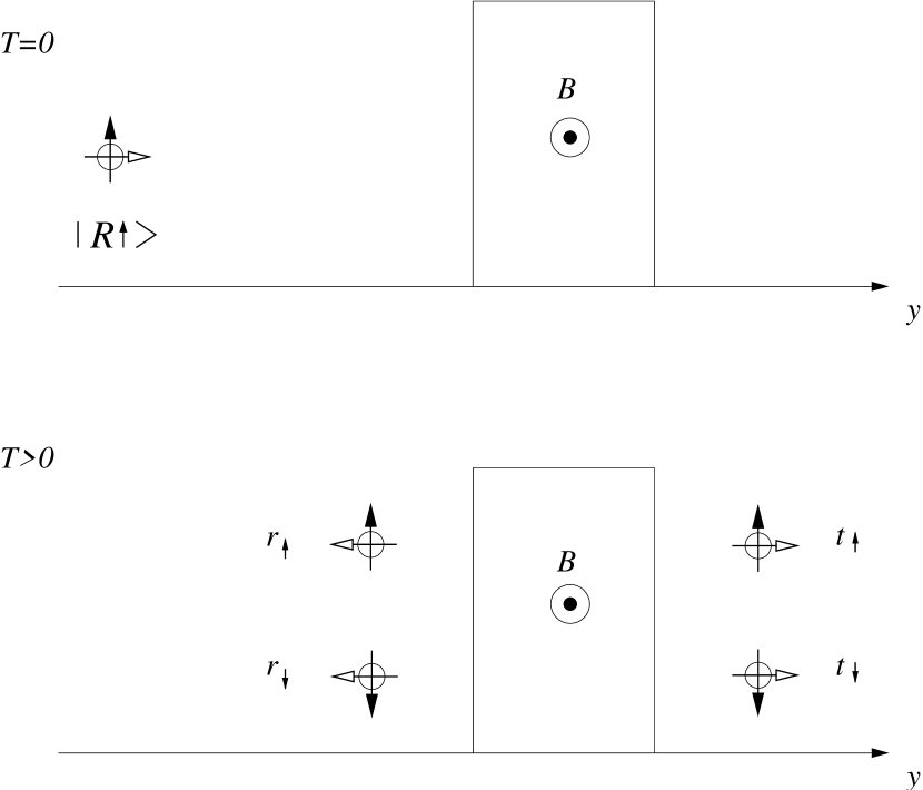
Figure 2: Transmission and reflection coefficients for a neutron initially prepared in the $|R\uparrow\rangle$ state.

These coefficients are connected with the energy levels by the following relation :

$$\pmatrix{t_{\uparrow}&t_{\downarrow}\cr r_{\uparrow}&r_{\downarrow}}=\frac{1}{4}\pmatrix{1&1\cr 1&-1}\pmatrix{e^{-iE_{++}T}&e^{-iE_{+-}T}\cr e^{-iE_{-+}T}&e^{-iE_{--}T}}\pmatrix{1&1\cr 1&-1}. 4.5$$ ()

By specifying the values of the parameters $g,\alpha,\beta$ and the total interaction time $T$, one univocally determines $t_{\uparrow},t_{\downarrow},r_{\uparrow}$ and $r_{\downarrow}$. Direct physical meaning can therefore be attributed to the constants $g,\alpha$ and $\beta$ in ($4.2$) by comparison with the transmission/reflection coefficients. For example, in order to mimic a realistic experimental setup with given values of $t_{\uparrow\downarrow},r_{\uparrow\downarrow}$, it is enough to obtain the values of $g,\alpha$ and $\beta$ from ($4.5$) and plug them in the Hamiltonian ($4.2$). The model could in principle be further improved by making the constant $g$ energy-dependent. We will consider a more realistic Hamiltonian in Sec. 6.

5 The ideal case of complete transmission

In the following discussions we always assume that our initial state is $|R\uparrow\rangle$, i.e., a right-going spin-up neutron, and consider, for definiteness, the case of total transmission with spin flipped, i.e., $|t_{\downarrow}|^{2}=1$, when no measurements are performed. Of course, this has to be considered as an idealized situation, since a spin rotation can only take place when there is an interaction potential (proportional to the intensity of the magnetic field) which necessarily produces reflection effects (with the only exception of plane waves). Stated differently, when the spatial degrees of freedom are taken into account in the scattering problem off a spin-flipping potential, complete transmission is impossible to achieve: There are always reflected waves. Our model Hamiltonian ($4.2$) must therefore be regarded as a simple caricature of the physical system we are analyzing. Wave packet effects will be discussed in Sec. 6.

To obtain a total transmission with spin flipped, the evolution operator should have the form $e^{-iHT}\propto\sigma_{1}$, which is equivalent to either

$$e^{-i\alpha gT\tau_{1}}\propto\tau_{1},\quad e^{-i\beta gT\sigma_{1}}\propto 1,\quad e^{-i\alpha\beta gT\tau_{1}\sigma_{1}}\propto\tau_{1}\sigma_{1}, 5.1$$ ()

$$e^{-i\alpha gT\tau_{1}}\propto 1,\quad e^{-i\beta gT\sigma_{1}}\propto\sigma_{1},\quad e^{-i\alpha\beta gT\tau_{1}\sigma_{1}}\propto 1.$$

That is,

$${\rm Case\ i)}\hfill \cos\alpha gT=\sin\beta gT=\cos\alpha\beta gT=0, 5.3$$ ()

$${\rm Case\ ii)}\hfill \sin\alpha gT=\cos\beta gT=\sin\alpha\beta gT=0. 5.4$$ ()

(All other cases, such as total reflection with/without spin-flip can be analyzed in a similar way.) In both cases, the evolution is readily computed:

$$e^{-iHT}|R\uparrow\rangle=\mbox{phase factor}\times|R\downarrow\rangle. 5.5$$ ()

The boundary conditions are such that the neutron is transmitted and its spin flipped with unit probability. For the experimental realization, see [16]. This is the situation outlined in Figure 1(a).

We shall now focus on some interesting cases, which illustrate some definite aspects of the QZE.  Let us see, in particular, how the evolution of the quantum state of the neutron is modified by choosing different projectors (corresponding to different “measurements”).

5.1 Direction-insensitive spin measurement

We perform now a series of measurements, in order to check whether the neutron spin is up. Let us call this type of measurement a “direction-insensitive spin measurement,” for reasons that will become clear later.

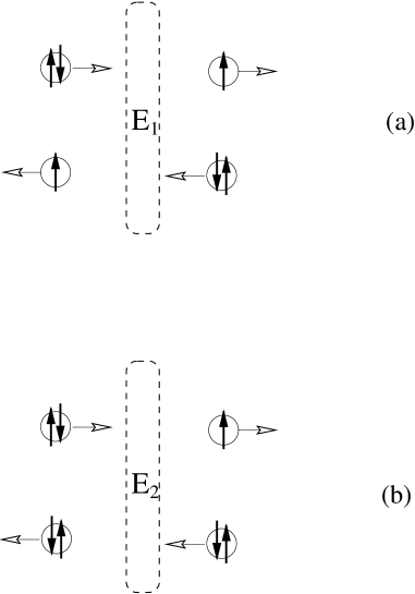
Figure 3: (a) Direction-insensitive spin measurement. (b) Direction-sensitive spin measurement.

Refer to Figure 3(a). The projection operator corresponding to this measurement is

$$E_{1}=1-|R\downarrow\rangle\langle R\downarrow|-|L\downarrow\rangle\langle L\downarrow|={1\over 2}(1+\sigma_{3}), 5.6$$ ()

that is, the spin-down components are projected out regardless of the direction of propagation of the neutron. In this case, after frequent measurements $E_{1}$ performed at time intervals $T/N$, the evolution operator in Eq. ($2.6$) reads

$$V_{N}(T)=\left(E_{1}e^{-iHT/N}E_{1}\right)^{N}=E_{1}(t_{\uparrow}+r_{\uparrow}\tau_{1})^{N}, 5.7$$ ()

where $t_{\uparrow}\sim 1-igT/N$ and $r_{\uparrow}\sim-i\alpha gT/N$ for large $N$ [see Eq. ($4.4$)]. Taking the limit, one obtains the following expression for the QZE evolution operator defined in Eq. ($2.8$):

$${\cal V}(T)=\lim_{N\to\infty}V_{N}(T)=e^{-igT}E_{1}e^{-i\alpha gT\tau_{1}}. 5.8$$ ()

Interesting physical situations can now be investigated. Choose, for instance, $gT=\pi,\alpha=-1/2,\beta=-1$, which belongs to Case i) in Eq. ($5.3$) [so that, without measurements, the neutron is totally transmitted with its spin flipped, as shown in Eq. ($5.5$)]. When the direction-insensitive measurements are continuously performed, the QZE evolution is ${\cal V}(T)=-iE_{1}\tau_{1}$ and the final state is

$${\cal V}(T)|R\uparrow\rangle=-i|L\uparrow\rangle, 5.9$$ ()

i.e., the neutron spin is not flipped, but the neutron itself is totally reflected. This clearly shows that reflection “losses” can be very important; as a matter of fact, reflection effects dominate, in this example. Notice that this is always an example of QZE: The projection operator $E_{1}$ in ($5.6$) prevents the spin from flipping. The point here is, however, that $E_{1}$ is not “tailored” so as to prevent the wave function from being reflected!

5.2 Another particular case: seminal model

Let us now focus on a model corresponding to Case ii) in Eq. ($5.4$). The choice of parameters, e.g. $gT=\pi/2,\alpha=2n,\beta=-1$, obviously fulfills these conditions for arbitrary integer $n$. Total transmission with spin flipped occurs again when no measurement is performed.

When direction-insensitive spin measurements, described by projections $E_{1}$, are performed at time intervals $T/N$ and in the $N\to\infty$ limit, the QZE evolution operator in Eq. ($5.8$) becomes simply ${\cal V}_{1}(T)=-i(-1)^{n}E_{1}$ and the final state is

$${\cal V}_{1}(T)|R\uparrow\rangle=-i(-1)^{n}|R\uparrow\rangle, 5.10$$ ()

so that the “usual” QZE is obtained. When $n=0$ this is our seminal model [8], reviewed in Sec. 3. Obviously, the case $n=0$ is not rich enough to yield information about reflection effects. In the following subsection the case of nonzero $n$ will be discussed.

5.3 Direction-sensitive spin measurements

We now consider a different type of spin measurement. Let the measurement be characterized by the following projection operator

$$E_{2}=1-|R\downarrow\rangle\langle R\downarrow|, 5.11$$ ()

which projects out those neutrons that are transmitted with their spin flipped. Notice that spin-down neutrons that are reflected are not projected out by $E_{2}$: for this reason we call this a “direction-sensitive” spin measurement. Refer to Figure 3(b). Even though the action of this projection is not easy to implement experimentally, this example clearly illustrates some interesting issues related to the Misra–Sudarshan theorem. We shall see that the action of the projector $E_{2}$ will yield a very interesting result. For large $N$, the evolution is given by

$$V_{2,N}(T)=\left(E_{2}e^{-iHT/N}E_{2}\right)^{N}=e^{-igT}\left(1-i\frac{gT}{N}Z\right)^{N}E_{2}+O(1/N), 5.12$$ ()

where $Z\equiv E_{2}(H/g-1)E_{2}$. The QZE evolution is given by the limit

$${\cal V}_{2}(T)=\lim_{N\to\infty}V_{2,N}(T)=e^{-igT}e^{-igTZ}E_{2}. 5.13$$ ()

To compute its effect on the initial state $|R\uparrow\rangle$, we note that, when acting on states $|R\uparrow\rangle,|L\uparrow\rangle$ and $|L\downarrow\rangle$, which span the “survival” subspace, the $Z$ operator behaves as

$$Z\left(\matrix{|R\uparrow\rangle\cr|L\uparrow\rangle\cr|L\downarrow\rangle}\right)=\left(\matrix{0&\alpha&\alpha\beta\cr\alpha&0&\beta\cr\alpha\beta&\beta&0}\right)\left(\matrix{|R\uparrow\rangle\cr|L\uparrow\rangle\cr|L\downarrow\rangle}\right). 5.14$$ ()

Let us choose for definiteness $\beta=-1$, so that

$$(Z-1/2)^{2}|R\uparrow\rangle=\theta^{2}|R\uparrow\rangle, 5.15$$ ()

with $\theta=\sqrt{8\alpha^{2}+1}/2$. Thus the final state can be readily obtained

$${\cal V}_{2}(T)|R\uparrow\rangle=e^{-3igT/2}\Biggl{[}\left(\cos gT\theta+\frac{i}{2\theta}\sin gT\theta\right)|R\uparrow\rangle+\frac{i\alpha}{\theta}\sin gT\theta\Bigl{(}|L\downarrow\rangle-|L\uparrow\rangle\Bigr{)}\Biggr{]}. 5.16$$ ()

Therefore, for a continuous direction-sensitive (namely, $E_{2}$) measurement, the probability of finding the initial state $|R\uparrow\rangle$ is not unity. Part of the wave function will be reflected, although the neutron would have been totally transmitted without measurement [see ($5.5$)] or with an “$E_{1}$-measurement” [see ($5.10$)].

Clearly, the action of the projector $E_{2}$ yields a completely different result from that of $E_{1}$, in ($5.10$). This is obvious and easy to understand: the state ($5.16$) belongs to the subspace of the “survived” states, according to the projection $E_{2}$. Notice also that the probability loss due the measurements is zero, in the limit, because the QZE evolution ($5.13$) is unitary within the subspace of the “survived” states.

6 A more realistic model

Let us now introduce a more realistic (albeit static) model. Such a model can be shown to be derivable from a Hamiltonian very similar to the one studied in the previous sections by a suitable identification of parameters (see Appendix A). The effect of reflections in the QZE will now be tackled by directly solving a stationary Schrödinger equation, which will be set up as follows.

Let a neutron with energy $E=k^{2}/2m$ and spin up ($+z$ direction), moving along the $+y$ direction, impinge on $N$ regions of constant magnetic field pointing to the $x$ direction, among which there are $N-1$ field-free regions. The thickness of a single piece of magnetic field is $a$ and the field-free region has size $b$. The configuration is shown in Figure 4.

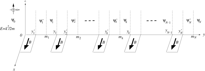
Figure 4: Spin-up neutron moving along the $+y$ direction with energy $E$. The magnetic field points to the $+x$ direction and is zero in the region between $y_{n}^{\prime}$ and $y_{n}$, in which the measurements will be made. In these field-free regions the wave functions are $|\psi_{n}^{\prime}\rangle$ before measurement and $|\psi_{n}\rangle$ after the measurement.

Thus we have the one-dimensional scattering problem of a neutron off a piecewise constant magnetic field with total thickness $D=Na$. The stationary Schrödinger equation is described by the Hamiltonian

$$H_{\rm Z}=\frac{p_{y}^{2}}{2m}+\mu B\sigma_{1}\Omega(y), 6.1$$ ()

where $\mu$ is the modulus of the neutron magnetic momentum, $B$ the strength of the magnetic field and

$$\Omega(y)=\left\{\matrix{0&\mbox{for}&y<0,&y_{n}^{\prime}<y<y_{n},&y_{N}^{\prime}<y&(n=1,2,\ldots,N),\cr\vskip 3.0pt plus 1.0pt minus 1.0pt\cr 1&\mbox{for}&&y_{n-1}<y<y_{n}^{\prime}&&(n=1,2,\ldots,N),\cr}\right. 6.2$$ ()

with $y_{n}=n(a+b)$ and $y_{n}^{\prime}=y_{n-1}+b$, characterizes the configuration of the magnetic field $B$ applied along the $x$-axis. Refer to Figure 4. The incident state of the neutron is taken to be $|\psi_{\rm in}\rangle=e^{iky}|\uparrow\rangle$. Let $r_{\uparrow(\downarrow)}$ be the reflection amplitude for the spin-up (spin-down) component. The wave function for $y<0$ is written as

$$|\psi_{0}\rangle=e^{iky}|\uparrow\rangle+e^{-iky}[r_{\uparrow}|\uparrow\rangle+r_{\downarrow}|\downarrow\rangle]. 6.3$$ ()

Denoting the transmission amplitudes for spin-up and spin-down as $t_{\uparrow}$ and $t_{\downarrow}$, the outgoing wave function in the region $y>y_{N}^{\prime}$ reads

$$|\psi_{N}\rangle=e^{iky}[t_{\uparrow}|\uparrow\rangle+t_{\downarrow}|\downarrow\rangle]. 6.4$$ ()

Since $[\sigma_{1},H_{\rm Z}]=0$, it is convenient to work with the basis $|\pm\rangle=(|\uparrow\rangle\pm|\downarrow\rangle)/\sqrt{2}$, i.e., the eigenstates of $\sigma_{1}$ belonging to eigenvalues $\pm 1$. For later use we denote $r_{\pm}=r_{\uparrow}\pm r_{\downarrow}$ and $t_{\pm}=t_{\uparrow}\pm t_{\downarrow}$.

In the field-free region, before the point $y=m_{n}$ where the $n$th measurement is assumed to take place, $y_{n}^{\prime}<y<m_{n}$, the wave function is

$$|\psi_{n}^{\prime}\rangle=\sum_{\sigma=\pm}\left(R^{\prime}_{n,\sigma}e^{ik(y-y^{\prime}_{n})}+L^{\prime}_{n,\sigma}e^{-ik(y-y^{\prime}_{n})}\right)|\sigma\rangle,\quad(n=1,2,\ldots,N). 6.5$$ ()

On the other hand, in the region after the $n$th measurement, $m_{n}<y<y_{n}$, the wave function is

$$|\psi_{n}\rangle=\sum_{\sigma=\pm}\left(R_{n,\sigma}e^{ik(y-y_{n})}+L_{n,\sigma}e^{-ik(y-y_{n})}\right)|\sigma\rangle,\quad(n=0,1,\ldots,N). 6.6$$ ()

The relation between the amplitudes of the wave functions $|\psi^{\prime}_{n+1}\rangle$ and $|\psi_{n}\rangle$ at the right- and left-hand sides of the $n$th potential region is determined by the boundary conditions at points $y_{n}$ and $y_{n}^{\prime}$. In fact, we have

$$\pmatrix{R^{\prime}_{n+1,\pm}\cr L^{\prime}_{n+1,\pm}}=M_{\pm}\pmatrix{R_{n,\pm}\cr L_{n,\pm}}, 6.7$$ ()

where the transfer matrix is given by

$$M_{\pm}=\pmatrix{\cos k_{\pm}a+i\cosh\eta_{\pm}\sin k_{\pm}a&-i\sinh\eta_{\pm}\sin k_{\pm}a\cr i\sinh\eta_{\pm}\sin k_{\pm}a&\cos k_{\pm}a-i\cosh\eta_{\pm}\sin k_{\pm}a} 6.8$$ ()

with $k_{\pm}=\sqrt{k^{2}\mp 2m\mu B}$ and $k/k_{\pm}=e^{\eta_{\pm}}$. This can also be expressed in a concise way in terms of the Pauli matrices in this two dimensional space, $\tau_{1}$, $\tau_{2}$ and $\tau_{3}$, as

$$M_{\pm}=e^{\eta_{\pm}(1+\tau_{1})/2}e^{ik_{\pm}a\tau_{3}}e^{-\eta_{\pm}(1+\tau_{1})/2}. 6.9$$ ()

We clearly see that the above formula contains all the boundary information at points $y_{n}$ and $y_{n}^{\prime}$: The first and last factors are the kicks exerted at the boundaries of a single piece of constant magnetic field, while the central one represents a free evolution with relative energy $E\mp\mu B$.

In what follows, we shall incorporate the measurement processes performed at points $m_{n}$ as some kind of boundary conditions, connecting the primed and unprimed wave functions in the field-free region.

6.1 Evolution without any spin measurements

We first consider the case where there is no measurement at all. This enables us to set up the notation and rederive some known results (which will be useful for future comparison). In this case the primed and unprimed wave functions must be equal $|\psi^{\prime}_{n}\rangle=|\psi_{n}\rangle$ in the field-free region. By virtue of Eq. ($6.7$) we obtain

$$\pmatrix{R_{n+1,\pm}\cr L_{n+1,\pm}}=e^{ikb\tau_{3}}M_{\pm}\pmatrix{R_{n,\pm}\cr L_{n,\pm}}. 6.10$$ ()

Notice the boundary conditions $R_{0,\pm}=1/\sqrt{2}$ and $L_{N,\pm}=0$ together with the definitions of transmission amplitude $R_{N,\pm}=e^{iky_{N}}t_{\pm}/\sqrt{2}$ and reflection amplitude $L_{0,\pm}=r_{\pm}/\sqrt{2}$. After applying the above equation $N$ times, we obtain the following relation

$$e^{iky_{N}}\pmatrix{t_{\pm}\cr 0\cr}=\left([N]_{\pm}e^{ikb\tau_{3}}M_{\pm}-[N-1]_{\pm}\right)\pmatrix{1\cr r_{\pm}\cr}, 6.11$$ ()

where $[N]_{\pm}=(q_{\pm}^{N}-q_{\pm}^{-N})/(q_{\pm}-q_{\pm}^{-1})$, with $q_{\pm},q_{\pm}^{-1}$ being the two eigenvalues of the transfer matrix $e^{ikb\tau_{3}}M_{\pm}$, which are determined by

$$\frac{q_{\pm}+q_{\pm}^{-1}}{2}=\cos kb\cos k_{\pm}a-\cosh\eta_{\pm}\sin kb\sin k_{\pm}a. 6.12$$ ()

When there is only a single piece of magnetic field with length $a$, i.e., $N=1$, the transmission amplitude of a neutron in the spin state $|\pm\rangle$ is

$$t_{a\pm}=\frac{e^{-ika}}{\cos k_{\pm}a-i\cosh\eta_{\pm}\sin k_{\pm}a}, 6.13$$ ()

as is well known. From Eq. ($6.11$), for an arbitrary $N>1$, the transmission amplitude of the same neutron passing through a magnetic field with a lattice-like structure as depicted in Figure 4 can be written as

$$t_{\pm}=\frac{e^{-iky_{N}}t_{a\pm}}{e^{-iky_{1}}[N]_{\pm}-[N-1]_{\pm}t_{a\pm}}. 6.14$$ ()

For a neutron in its spin-up state $|\uparrow\rangle$, the transmission amplitude with spin unflipped is then $t_{\uparrow}=(t_{+}+t_{-})/2$ and that with spin flipped is $t_{\downarrow}=(t_{+}-t_{-})/2$. As a result, for a spin-up neutron to go through a constant potential of width $y_{N}=D=Na$ without reflection and with spin flipped, i.e., $|t_{\downarrow}|=1$, one should require $k_{\pm}D=n_{\pm}\pi$ or

$$E=\frac{\pi^{2}(n_{+}^{2}+n_{-}^{2})}{4mD^{2}},\quad\mu B=\frac{\pi^{2}(n_{+}^{2}-n_{-}^{2})}{4mD^{2}}, 6.15$$ ()

with $n_{\pm}$ two arbitrary integers, their difference $n_{+}-n_{-}$ being an odd number. In this case of complete transmission $|t_{\downarrow}|=1$, the energy $E$ must be larger than the potential $\mu B$. The rest of the analysis above, however, is valid also when the energy is less than the potential.

Now we consider the case where $N$ tends to infinity and the magnetic field possesses a periodic lattice structure. The relation ($6.10$) still holds and in order to preserve the translational symmetry along the $y$ axis (that is, to keep the Hamiltonian invariant under a translation of $(a+b)$ along the $y$-axis), one should have $|q_{\pm}|=1$ owing to the Bloch theorem. Equivalently, the trace of the transfer matrix $e^{ikb\tau_{3}}M_{\pm}$ as given in Eq. ($6.12$) should be less than one. This determines the energy band of the system: those energies that make the absolute value of this trace greater than 1 will be forbidden, because for these energies $|q_{\pm}|$ or $|q_{\pm}|^{-1}$ becomes larger than one and $[N]_{\pm}$ tends exponentially to infinity when $N$ approaches infinity. For large $N$, even if there is no periodical structure, there is always some $k$ that makes this trace greater than one (e.g. $kb+k_{\pm}a=l\pi$). Therefore the transmission probability will tend to zero exponentially when $N$ becomes large, even though the energy may be very large relative to the potential. This shows that reflection effects in presence of a lattice structure are very important; as we shall see, this feature is preserved even when projection operators are interspersed in the lattice.

6.2 Direction-insensitive projections

We consider now the second situation, when direction-insensitive measurements are performed at points $m_{n}$s. By this kind of measurement, the spin-down components are projected out and the spin-up components evolve freely regardless whether the neutron is travelling right or left.

The boundary conditions imposed by this kind of measurement at point $m_{n}$ for the wave function $|\psi_{n}\rangle$ and $|\psi^{\prime}_{n}\rangle$ in the field-free region are expressed as

$$R_{n,\downarrow}=L^{\prime}_{n,\downarrow}=0,\quad\pmatrix{R_{n,\uparrow}^{\prime}\cr L_{n,\uparrow}^{\prime}\cr}=e^{-ikb\tau_{3}}\pmatrix{R_{n,\uparrow}\cr L_{n,\uparrow}\cr}, 6.16$$ ()

where $R_{n,\uparrow}=(R_{n,+}+R_{n,-})/2$ and $R_{n,\downarrow}=(R_{n,+}-R_{n,-})/2$ for right-going components and similar expressions for the left-going and primed components. Therefore, application of Eq. ($6.7$) $N$ times yields

$$\pmatrix{R_{N,\uparrow}\cr L_{N,\uparrow}\cr}=(e^{ikb\tau_{3}}M_{1})^{N}\pmatrix{R_{0,\uparrow}\cr L_{0,\uparrow}\cr}, 6.17$$ ()

where the $2\times 2$ transfer matrix $M_{1}$ has the following matrix elements

$$(M_{1})_{ij}=\bar{M}_{ij}-\Delta M_{i2}\Delta M_{2j}/\bar{M}_{22} 6.18$$ ()

with $\bar{M}=(M_{+}+M_{-})/2$ and $\Delta M=(M_{+}-M_{-})/2$.

Now we take the limit as required by a “continuous” measurement, i.e., $N\to\infty$, $a\to 0$ keeping $Na=D$ finite and $Nb\to 0$. By the definition ($6.8$) of the transfer matrix, we have the small-$a$ expansions

$$\bar{M}=1+ika\tau_{3}+O(a^{2}),\quad\Delta M=\zeta ka(\tau_{2}-i\tau_{3})+O(a^{2}) 6.19$$ ()

with $\zeta\equiv\mu B/2E$, obtaining

$$\lim_{N\to\infty}(e^{ikb\tau_{3}}M_{1})^{N}=e^{ikD\tau_{3}}. 6.20$$ ()

Recall that $t_{\uparrow}=e^{-ikD}R_{N,\uparrow}$ is the transmission amplitude, $L_{0,\downarrow}=r_{\downarrow}$ the reflection amplitude and $L_{N,\uparrow}=0$ and $R_{0,\uparrow}=1$ because of the boundary conditions. After taking the limit $N\to\infty$ in Eq. ($6.17$), we see that the transmission (survival) probability becomes one, i.e., $|t_{\uparrow}|^{2}=1$, for any input energy and magnetic field. This reveals another aspect of neutron QZE: When the energy of the neutron is smaller than the potential, the transmission probability decays exponentially when the length increases and no measurement is performed; By contrast, when continuous direction-insensitive measurements are made, one can obtain a total transmission!

If we choose the energy of the neutron and the potential as in Eq. ($6.15$), without measurements the neutron will be totally transmitted with its spin flipped. On the other hand, if the spin-up state is measured continuously, the neutron will be totally transmitted with its spin unflipped. This is exactly the QZE in the usual sense. Our analysis enables us to see that two kinds of QZEs are taking place: One is the QZE for the right-going neutron, by which we obtain a total transmission of the right-going input state, and another one is for the left-going neutron, which preserves the zero amplitude of the left-going input state. This case corresponds to projector $E_{1}$ in our simplified model in Sec. 5.2.

6.3 Direction-sensitive projections

The third case we consider is the direction-sensitive measurement. By this kind of measurement the left-going components (or the reflection parts) evolve freely, no matter whether spin is up or down, and the right-going components are projected to the spin-up state. The corresponding boundary conditions are

$$R_{n,\downarrow}=0,\qquad L_{n,\pm}=e^{-ikb}L^{\prime}_{n,\pm}. 6.21$$ ()

If we apply Eq. ($6.7$) $N$ times, supplemented with these boundary conditions, the following relations among the transmission and reflection amplitudes are obtained

$$e^{ikD}\pmatrix{t_{\uparrow}\cr 0\cr 0}=\left(e^{ikb\Sigma_{3}}M_{2}\right)^{N}\pmatrix{1\cr r_{\uparrow}\cr r_{\downarrow}}, 6.22$$ ()

where $\Sigma_{3}$ is a diagonal matrix $\Sigma_{3}={\rm diag}\{1,-1,-1\}$ and the $3\times 3$ transfer matrix $M_{2}$ is given by

$$M_{2}=\pmatrix{\bar{M}_{11}&\bar{M}_{12}&\Delta M_{12}\cr\bar{M}_{21}&\bar{M}_{22}&\Delta M_{22}\cr\Delta M_{21}&\Delta M_{22}&\bar{M}_{22}\cr}. 6.23$$ ()

In the limit of continuous measurements ($N\to\infty$, $a\to 0$, while keeping $D=Na$ constant, and $Nb\to 0$), the transfer matrix is expanded as

$$M_{2}=1-ika/3+ikaZ_{2}+O(a^{2}), 6.24$$ ()

for small $a$, with ($\zeta=\mu B/2E$)

$$Z_{2}\equiv\pmatrix{4/3&0&-\zeta\cr 0&-2/3&\zeta\cr\zeta&\zeta&-2/3\cr}, 6.25$$ ()

and we have

$$\lim_{N\to\infty}(e^{ikb\Sigma_{3}}M_{2})^{N}=e^{-ikD/3}e^{ikDZ_{2}}. 6.26$$ ()

Notice that the matrix $Z_{2}$ satisfies $\Sigma_{3}Z_{2}\Sigma_{3}=Z_{2}^{\dagger}$, from which we obtain, in the above limit, the conservation of probability

$$|t_{\uparrow}|^{2}+|r_{\uparrow}|^{2}+|r_{\downarrow}|^{2}=1. 6.27$$ ()

This shows that there are no losses caused by the continuous direction-sensitive measurements. On the other hand, the transmission amplitude with spin unflipped is explicitly given by

$$t_{\uparrow}={{e^{-i4kD/3}}\over\left(e^{-ikDZ_{2}}\right)_{11}}, 6.28$$ ()

which implies that the transmission probability $|t_{\uparrow}|^{2}$ is in general not equal to one. To have a general impression of its behavior, we plot $T_{\uparrow}=|t_{\uparrow}|^{2}$ as a function of $kD$ and $\zeta$ in Figure 5.

Some comments are in order. There are two critical values for $\zeta$, namely $0$ and $\zeta_{c}=4\sqrt{3}/9\approx 0.77$. When $0\leq\zeta<\zeta_{c}$, the matrix $Z_{2}$ has three real eigenvalues and the transmission probability will oscillate depending on $kD$. When $\zeta=\zeta_{c}$ the transmission probability will decay according to $(kD)^{-2}$. In fact, if one defines $G=Z_{2}-2/3$, it is easy to show that $e^{-ikDG}=1-ikDG+(e^{2ikD}-1-2ikD)G^{2}/4$, because $G$ satisfies $G^{2}(G+2)=0$. Then one can explicitly confirm that the element $(e^{-ikDG})_{11}$ includes a linear $kD$ term, which gives the $(kD)^{-2}$ behavior to the transmission probability. Finally, when $\zeta>\zeta_{c}$ the matrix $Z_{2}$ has two imaginary eigenvalues and therefore the transmission probability decays exponentially with $kD$. This can be seen clearly in Figure 5(a). An interesting case arises when we consider $1/2<\zeta<\zeta_{c}$ or $E<\mu B<8\sqrt{3}E/9\approx 1.5E$. Without measurements, the transmission probability decays exponentially when the length of the magnetic field is increased, because the input energy is smaller than the potential. When continuous measurements are performed, however, the transmission probability will oscillate as the length of the magnetic field increases.

Figure 5: The transmission probability with spin unflipped $T_{\rm up}=|t_{\uparrow}|^{2}$ is plotted as a function of $kD$ and $z=\zeta$ in (a) and as a function of $B_{1}=\sqrt{m\mu B}D$ and $kD$ in (b).

As we can see in Figure 6, although the conditions ($6.15$) for total transmission in absence of measurements have been imposed, the transmission probability $T_{\uparrow}$ is not one, as it would be for the “ordinary” QZE. Reflections are unavoidable. This case corresponds to the projector $E_{2}$ considered in the simplified model.

Figure 6: The transmission probablity with spin unflipped $T_{\uparrow}=|t_{\uparrow}|^{2}$ as a function of $n$, when the conditions ($6.15$) for total transmission are satisfied with $n_{-}=n$ and $n_{+}=n+9$.

As we have seen, there are peculiar reflection effects in presence of projections, when $D$ (total length) is varied. This is clearly an interference effect, which can lead to enhancement of reflection “losses,” if the “projection” does not suppress the left component of the wave (this is what happens for $E_{2}$). This proves that reflection effects can become very important in experimental tests of the QZE with neutron spin, if, roughly speaking, the total length of the interaction region “resonates” with the neutron wavelength. It is interesting that such a resonance effect takes place even though the dynamical properties of the system are profoundly modified by the projection operators, in the limit of “continuous” measurements, leading to the QZE.

Finally, we would like to stress again that we are performing an analysis in terms of stationary states (i.e., transmission/reflection coefficients for plane waves), while at the same time we are analyzing a quantum Zeno phenomenon, which is essentially a time-dependent effect. This is meaningful within our approximations, where the wave-packet spread is neglected and the measurements are performed with very high frequency. A more sophisticated argument in support of this view is given in Appendix A. In the present context wave packets effects, if taken into account, would result in a sort of average of the effects shown in Figures 5 and 6 (which refer to the monochromatic case); however, our general conclusions would be unaltered. It is worth stressing that, in neutron optics, effects due to a high sensitivity to fluctuation phenomena (such as fluctuations of the intensity of the magnetic field) become important at high wave number and constitute an experimental challenge [17].

7 Summary

We have analyzed some peculiar features of a quantum Zeno-type dynamics by discussing the noteworthy example of a neutron spin evolving under the action of a magnetic filed in presence of different types of measurements (“projections”).

The “survival probability” depends on our definition of “surviving,” i.e., on the choice of the projection operator $E$. Different $E$s will yield different final states, and Misra and Sudarshan’s theorem [2] simply makes sure that the survival probability is unity: the final state belongs to the subspace of the survived products.

In the physical case considered (neutron spin), our examples clarify that the practical details of the experimental procedure by which the neutron spin is “measured” are very important. For example, in order to avoid constructive interference effects, leading to (unwanted) enhancement of the reflected neutron wave, it is important to devise the experimental setup in such a way that reflection effects are suppressed.

Appendix A

In this appendix, we shall endeavor to establish a connection between the models analyzed in Secs. 4 and 6. In other words, we will examine whether the parametrization of the Hamiltonian of the form ($4.2$) is compatible with the more realistic one considered in ($6.1$) and in such a case find which values are to be assigned to the parameters $\alpha,\beta$ and $g$. To this end, it is enough to consider the scattering (i.e., the transmission and reflection) process of a neutron off a single constant magnetic field $B$ of width $a$. We compare the scattering amplitudes calculated on the basis of the simple abstract Hamiltonian ($4.2$) and of the more realistic one ($6.1$). Notice that the process is treated as a dynamical one in the former case ($T$ is regarded, roughly speaking, as the time necessary for the neutron to go through the potential), while in the latter case we treat it as a stationary problem.

Observe first that the tranfer matrix $M_{\pm}$ in ($6.8$), derived for the stationary scattering process, yields the following transmission/reflection amplitudes

$$R^{\prime}_{1,\uparrow}={1\over 2}\left({1\over(M_{+})_{22}}+{1\over(M_{-})_{22}}\right), R^{\prime}_{1,\downarrow}={1\over 2}\left({1\over(M_{+})_{22}}-{1\over(M_{-})_{22}}\right),$$

$$L_{0,\uparrow}=-{1\over 2}\left({(M_{+})_{21}\over(M_{+})_{22}}+{(M_{-})_{21}\over(M_{-})_{22}}\right), L_{0,\downarrow}=-{1\over 2}\left({(M_{+})_{21}\over(M_{+})_{22}}-{(M_{-})_{21}\over(M_{-})_{22}}\right).$$

It is easy to show that the relations (LABEL:eq:RRLL) are equivalent to

$$\left(\begin{array}[]{cccc}1&1&1&1\\ 1&-1&1&-1\\ 1&1&-1&-1\\ 1&-1&-1&1\end{array}\right)\left(\begin{array}[]{c}R^{\prime}_{1,\uparrow}\\ R^{\prime}_{1,\downarrow}\\ L_{0,\uparrow}\\ L_{0,\downarrow}\end{array}\right)=\left(\begin{array}[]{c}{\cal M}_{-,+}\\ {\cal M}_{-,-}\\ {\cal M}_{+,+}\\ {\cal M}_{+,-}\end{array}\right),$$ (A.2)

where we have introduced

$${\cal M}_{+,\pm}={1+(M_{\pm})_{21}\over(M_{\pm})_{22}},\quad{\cal M}_{-,\pm}={1-(M_{\pm})_{21}\over(M_{\pm})_{22}}.$$ (A.3)

It is important to realize that these quantities are just phase factors. In fact, since

$$(M_{\pm})_{21}=i\sinh\eta_{\pm}\sin k_{\pm}a\quad\mbox{and}\quad(M_{\pm})_{22}=\cos k_{\pm}a-i\cosh\eta_{\pm}\sin k_{\pm}a$$ (A.4)

and

$$|1\pm(M_{\pm})_{21}|^{2}=|(M_{\pm})_{22}|^{2}=1+\sinh^{2}\eta_{\pm}\sin^{2}k_{\pm}a,$$ (A.5)

their absolute values are unity. Thus we can rewrite them in the form

$${\cal M}_{+,\pm}=e^{i(\xi_{\pm}+\phi_{\pm})},\quad{\cal M}_{-,\pm}=e^{i(-\xi_{\pm}+\phi_{\pm})},$$ (A.6)

where

$$\xi_{\pm}=\tan^{-1}(\sinh\eta_{\pm}\sin k_{\pm}a)\quad\mbox{and}\quad\phi_{\pm}=\tan^{-1}(\cosh\eta_{\pm}\tan k_{\pm}a).$$ (A.7)

Observe now that ($4.5$), dynamically derived from the abstract Hamiltonian ($4.2$), is equivalent to

$$\left(\matrix{t_{\uparrow}\cr t_{\downarrow}\cr r_{\uparrow}\cr r_{\downarrow}\cr}\right)={1\over 4}\left(\matrix{1&1&1&1\cr 1&-1&1&-1\cr 1&1&-1&-1\cr 1&-1&-1&1\cr}\right)\left(\matrix{e^{-iE_{++}T}\cr e^{-iE_{+-}T}\cr e^{-iE_{-+}T}\cr e^{-iE_{--}T}\cr}\right).$$ (A.8)

The apparent similarity between the above relation and (A.2), valid in the stationary scattering setup, induces us to look for a more definite connection between the two cases.

If we slightly generalize the abstract Hamiltonian ($4.2$)

$$H_{\rm dyn}=g[1+\alpha\tau_{1}+\beta\sigma_{1}+\gamma\tau_{1}\sigma_{1}],$$ (A.9)

by introducing the additional parameter $\gamma$, we easily find the correspondence existing between the parameters involved: The incident wave number $k$ of the neutron and the configuration of the static potential (strength $B$ and width $a$) determine the scattering data, which are reproducible by an appropriate choice of parameters $\alpha,\beta,\gamma$ and $gT$ in the dynamical process governed by the Hamiltonian (A.9).

For definiteness, consider the case of narrow potential, that is, $a\to 0$ or $ka\ll 1$. Incidentally, notice that this is the case of interest for the analysis of the QZE. The above $\xi_{\pm}$ and $\phi_{\pm}$ are then approximated as

$$\xi_{\pm}\sim\pm\zeta ka,\qquad\phi_{\pm}\sim(1\mp\zeta)ka,$$ (A.10)

where we set $\zeta=\mu B/2E=m\mu B/k^{2}$, as in Sec. 6. In the limit $a\to 0$, the evolution time $T$ is also considered to be of the same order of $a$ and the transmission and reflection coefficients are expressed, in terms of the parameters $\alpha,\beta,\gamma$ and $gT$, as

$$\left(\matrix{t_{\uparrow}\cr t_{\downarrow}\cr r_{\uparrow}\cr r_{\downarrow}\cr}\right)\sim\left(\matrix{1\cr-i\beta gT\cr-i\alpha gT\cr-i\gamma gT\cr}\right).$$ (A.11)

In the stationary scattering problem, the same quantities are calculated to be

$$\left(\matrix{t_{\uparrow}\cr t_{\downarrow}\cr r_{\uparrow}\cr r_{\downarrow}\cr}\right)=\left(\matrix{e^{-ika}R^{\prime}_{1,\uparrow}\cr e^{-ika}R^{\prime}_{1,\downarrow}\cr L_{0,\uparrow}\cr L_{0,\downarrow}\cr}\right)\sim\left(\matrix{1-ika+i(\phi_{+}+\phi_{-})/2\cr i(\phi_{+}-\phi_{-})/2\cr-i(\xi_{+}+\xi_{-})/2\cr-i(\xi_{+}-\xi_{-})/2\cr}\right)\sim\left(\matrix{1\cr-i\zeta ka\cr 0\cr-i\zeta ka\cr}\right).$$ (A.12)

Therefore, the following abstract Hamiltonian

$$H_{\rm dyn}=\mu B(1+\tau_{1})\sigma_{1}$$ (A.13)

can reproduce the desired scattering data when the system evolves under this Hamiltonian for time $T=a/v=ma/k$.

It is also interesting to see how such a dynamical Hamiltonian $H_{\rm dyn}$ may reproduce the transfer matrix $M_{\pm}$ ($6.8$), which further confirms the equivalence between the two formalisms, stationary and dynamical, governed by the Hamiltonians $H_{\rm Z}$ and $H_{\rm dyn}$, respectively. For this purpose, consider first a neutron, initially prepared in state $|R\pm\rangle$, subject to the dynamical evolution engendered by $H_{\rm dyn}$ for time $T=ma/k$. By definition, the transfer matrix connects the scattering products in the following way

$$\pmatrix{R_{1,\pm}^{\prime}\cr 0\cr}=M_{\pm}\pmatrix{1\cr L_{0,\pm}\cr}.$$ (A.14)

These scattering amplitudes are given by the corresponding matrix elements of the evolution operator $e^{-iHT}$,

$$e^{-ika}R_{1,\pm}^{\prime}=\langle R\pm|e^{-iHT}|R\pm\rangle,\qquad L_{0,\pm}=\langle L\pm|e^{-iHT}|R\pm\rangle,$$ (A.15)

which reduces, for small $T$, to

$$R_{1,\pm}^{\prime}\sim 1+ika\mp i\mu BT,\qquad L_{0,\pm}\sim\mp i\mu BT.$$ (A.16)

On the other hand, if a neutron is prepared in $|L\pm\rangle$, we have the relation

$$\pmatrix{R_{1,\pm}^{\prime}\cr e^{-ika}\cr}=M_{\pm}\pmatrix{0\cr L_{0,\pm}\cr},$$ (A.17)

where

$$R_{1,\pm}^{\prime}=e^{ika}\langle R\pm|e^{-iHT}|L\pm\rangle\sim\mp i\mu BT,\qquad L_{0,\pm}=\langle L\pm|e^{-iHT}|L\pm\rangle\sim 1\mp i\mu BT.$$ (A.18)

It is now an easy task to determine the matrix elements of $M_{\pm}$ from the above relations (A.14)–(A.18). We obtain

$$M_{\pm}\sim\pmatrix{1+ika\mp i\mu BT&\mp i\mu BT\cr\pm i\mu BT&1-ika\pm i\mu BT}=1-i[\pm\mu B(i\tau_{2}+\tau_{3})-2E\tau_{3}]T.$$ (A.19)

By defining a “generator” $G_{\rm d}$

$$G_{\rm d}=\mu B(i\tau_{2}+\tau_{3})\sigma_{1}-2E\tau_{3},$$ (A.20)

the transfer matrix $M_{\pm}$ for finite $a$ (or $T$) can be rewritten as

$$M_{\pm}=\langle\pm|e^{-iG_{\rm d}T}|\pm\rangle,$$ (A.21)

which is nothing but the transfer matrix ($6.8$), obtained for the stationary-state problem from the Hamiltonian $H_{\rm Z}$.

References

- [1] A. Beskow and J. Nilsson, Arkiv für Fysik 34 (1967) 561; L.A. Khalfin, Zh. Eksp. Teor. Fiz. Pis. Red. 8 (1968) 106 [JETP Letters 8 (1968) 65]; Phys. Lett. 112B (1982) 223; Usp. Fiz. Nauk 160 (1990) 185 [Sov. Phys. Usp. 33 (1990) 10]; L. Fonda, G.C. Ghirardi, A. Rimini and T. Weber, Nuovo Cim. A15 (1973) 689; A18 (1973) 805; A. De Gasperis, L. Fonda and G.C. Ghirardi, Nuovo Cim. A21 (1974) 471.
- [2] B. Misra and E.C.G. Sudarshan, J. Math. Phys. 18 (1977) 756.
- [3] For a review on the temporal behavior of quantum systems and the quantum Zeno effect, see L. Fonda, G.C. Ghirardi and A. Rimini, Rep. Prog. Phys. 41 (1978) 587; G-C. Cho, H. Kasari and Y. Yamaguchi, Prog. Theor. Phys. 90 (1993) 803; H. Nakazato, M. Namiki and S. Pascazio, Int. J. Mod. Phys. B10 (1996) 247; D. Home and M.A.B. Whitaker, Ann. Phys. 258 (1997) 237.
- [4] The first experimental observation of non-exponential decay at short times for an unstable system was performed two years ago: S.R. Wilkinson et al., Nature 387 (1997) 575. No attempt has yet been made to suppress decay by repeated measurements (quantum Zeno effect).
- [5] R.J. Cook, Phys. Scr. T21 (1988) 49.
- [6] W.H. Itano, D.J. Heinzen, J.J. Bollinger and D.J. Wineland, Phys. Rev. A41 (1990) 2295.
- [7] T. Petrosky, S. Tasaki and I. Prigogine, Phys. Lett. A151 (1990) 109; Physica A170 (1991) 306; A. Peres and A. Ron, Phys. Rev. A42 (1990) 5720; L.E. Ballentine, Phys. Rev. A43 (1991) 5165; W.H. Itano, D.J. Heinzen, J.J. Bollinger and D.J. Wineland, Phys. Rev. A43 (1991) 5168; V. Frerichs and A. Schenzle, in Foundations of Quantum Mechanics, T.D. Black, M.M. Nieto, H.S. Pilloff, M.O. Scully and R.M. Sinclair, eds. (World Scientific, Singapore, 1992); S. Inagaki, M. Namiki and T. Tajiri, Phys. Lett. A166 (1992) 5; D. Home and M.A.B. Whitaker, J. Phys. A25 (1992) 657; Phys. Lett. A173 (1993) 327; Ph. Blanchard and A. Jadczyk, Phys. Lett. A183 (1993) 272; T.P. Altenmuller and A. Schenzle, Phys. Rev. A49 (1994) 2016; L.S. Schulman, A. Ranfagni and D. Mugnai, Phys. Scr. 49 (1994) 536; M. Berry, in Fundamental Problems in Quantum Theory, eds., D.M. Greenberger and A. Zeilinger (Ann. N.Y. Acad. Sci. Vol. 755, New York, 1995), p. 303; A. Beige and G. Hegerfeldt, Phys. Rev. A53 (1996) 53; A. Luis and J. Periňa, Phys. Rev. Lett. 76 (1996) 4340. H. Nakazato, M. Namiki, S. Pascazio and H. Rauch, Phys. Lett. A217 (1996) 203; L.S. Schulman, J. Phys. A30 (1997) L293; Phys. Rev. A57 (1998) 1509. K. Thun and J. Periňa, Phys. Lett. A249 (1998) 363.
- [8] S. Pascazio, M. Namiki, G. Badurek and H. Rauch, Phys. Lett. A179 (1993) 155; S. Pascazio and M. Namiki, Phys. Rev. A50 (1994) 4582.
- [9] P. Kwiat, H. Weinfurter, T. Herzog, A. Zeilinger and M. Kasevich, Phys. Rev. Lett. 74 (1995) 4763.
- [10] H. Nakazato, M. Namiki, S. Pascazio and H. Rauch, Phys. Lett. A199 (1995) 27; Z. Hradil, H. Nakazato, M. Namiki, S. Pascazio and H. Rauch, Phys. Lett. A239 (1998) 333.
- [11] J. von Neumann, Die Mathematische Grundlagen der Quantenmechanik (Springer, Berlin, 1932). [English translation by E.T. Beyer: Mathematical Foundation of Quantum Mechanics (Princeton University Press, Princeton, 1955)]. For the QZE, see in particular p. 195 of the German edition (p. 366 of the English translation).
- [12] E.P. Wigner, Am. J. Phys. 31 (1963) 6.
- [13] Misra and Sudarshan in [2] considered an initial “unstable” state and took to be the subspace of the undecayed states. The expression “survived” means in their case “undecayed.”
- [14] A. Peres, Am. J. Phys. 48 (1980) 931.
- [15] E. Jericha, C.J. Carlile, M. Jaekel and H. Rauch, Physica B234-236 (1997) 1066.
- [16] B. Alefeld, G. Badurek and H. Rauch, Z. Phys. 41B (1981) 231.
- [17] H. Rauch, M. Suda and S. Pascazio, “Decoherence, dephasing and depolarization” Physica B, in print; G. Badurek, H. Rauch, M. Suda and H. Weinfurter, “Identification of a coherent superposition of spin-up and spin-down states in neutron spin-echo systems” preprint 1999.