Characterizing teleportation in optics

Abstract

We discuss the characterization of continuous variable, optical quantum teleportation in terms of the two quadrature signal transfer and conditional variances between the input and output states. We derive criteria which clearly define the classical limits and highlight interesting operating points which are not obvious from a calculation of the fidelity of the teleportation alone.

(3rd February 1999)

I Introduction

The quantum state of a system may be transmitted from one location to another through the direct transmission of only classical information provided, the sender and receiver share a non-locally entangled state of the Einstein, Podolsky, Rosen (EPR) type [1]. This process is called quantum teleportation and was first described in the context of spin-$1/2$ particles by Bennett et al. [2]. The first experimental realizations [3, 4] teleported single photon states, albeit with very low efficiency. More recently Vaidman [5] and Braunstein and Kimble [6] have proposed teleportation of continuous quantum variables, such as the quadrature amplitudes of the electromagnetic field. A high efficiency experimental demonstration of this technique has been made by Furusawa et al [7] using parametric down conversion as an EPR source [8].

Teleportation has applications in quantum computing [9] and general quantum information manipulation [10]. Continuous variable teleportation can be applied both through continuous variable generalizations of discrete manipulations [11] and continuous variable manipulations of discrete properties [12]. Teleportation of optical fields holds great promise due to the power of the required optical tools and the maturity of relevant optical communications technology.

With these experiments performed and more no doubt planned the issue of how to assess the experimental results arises. Traditionally teleportation is quantified by the fidelity [13] of the process. If the input is in the state $|\phi\rangle$ and the output is described by the density operator $\rho$ then the fidelity is given by $F=\langle\phi|\rho|\phi\rangle$. Fidelity is a measure of the overlap of the input and output states. In a general experiment one could completely characterize the input and output states individually via optical homodyne tomographic techniques [14] and thus calculate the fidelity. However most experimentally realizable optical states have Gaussian statistics and can therefore be fully characterized by measurements of the first and second order moments of orthogonal quadrature amplitudes, such as the amplitude and phase quadratures. For a particular set of input states a maximum fidelity which can be achieved without the use of entanglement can be derived. For coherent input states this maximum fidelity is $F=0.5$. This was exceeded in the Furusawa et al experiment [7].

On the other hand in the experiments of Boumeester [3] and Boschi [4] the fidelity was very low due to the low efficiency of the teleportation. In spite of this (or perhaps, as we shall see, because of this) strong quantum mechanical correlations in the form of non-local entanglement were preserved in the teleportation process. This suggests that fidelity alone does not give the entire picture with regard to the teleportation of particular quantum mechanical properties. Further, fidelity does not neccessarily recognize the similarity of states which differ only by reversible transformations. This is important because the desired quantum information may be preserved in such transformations. If a reversibly transformed version of the input state emerged from a teleportation process a measure of the fidelity may indicate lack of success when, in fact, the desired result has been achieved. These examples suggest that additional measures are required to fully characterize the teleportation process. In this paper we examine the teleportation criteria proposed by Ralph and Lam [15]. These criteria are based specifically on the similarity of measurement results obtained from the input and output of the teleporter, rather than the inferred similarity of the input and output states. We discuss, with examples, how the above problems are handled by these criteria.

II The Classical Limits

The criteria are two-dimensional and, in analogy with the quantum non-demolition measurement (QND) criteria [16], are based on the information transfer and quantum correlation achieved by the teleportation. Unlike QND, both quadratures of the teleported beam are considered. By examining the limits imposed on these quantities in any classical transmission scheme criteria for defining quantum teleportation are derived. The criteria are based on second order moments of the field which are straightforward to measure.

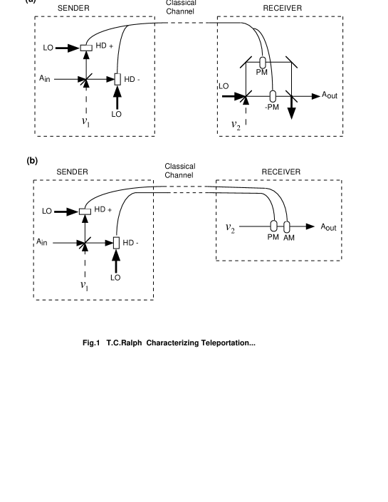
Figure 1: Schematic of classical teleportation arrangements. The arrangement in (a) is an idealized, general one which can in principle cope with any intensity of the input field. The arrangement in (b) can be used if the coherent amplitude of the input beam is large compared to the quantum fluctuations and is the one discussed in detail in this paper. Symbols are; LO:local oscillator, HD+:homodyne detection of the amplitude quadrature, HD-:homodyne detection of the phase quadrature, PM:phase modulation, -PM:phase modulation $\pi$ out of phase, AM:amplitude modulation, $v_{1}$:vacuum input. In (a) $v_{2}$:vacuum input, in (b) $v_{2}$:coherent field with a coherent amplitude equal to that of the input.

In Fig. 1 we show a “classical teleportation” scheme. By classical teleportation we mean that only classical channels are used and no entanglement is involved. An input field, in a minimum uncertainty state, is detected and the classical information collected is sent to a remote station. There the information is used to try to reconstruct the original beam. Two possible reconstruction schemes are shown. An idealized general method (Fig.1(a)) is to use a Mach-Zender arrangement with phase modulators in each arm introducing the same transmitted signal but with a $\pi$ phase shift between them. On the other hand if the input beam is bright, simpler direct amplitude and phase modulation of a receiver beam can be used (Fig.1(b)). In this case the average coherent amplitude of the input beam can be regarded as a classical quantity. We will concentrate on this latter case in developing the criteria. We consider an input beam of the form

$$\hat{A}_{\rm in}(t)=A_{\rm in}+\delta\hat{A}_{\rm in}(t)$$ (1)

where $\hat{A}_{\rm in}$ is the field annihilation operator; $A_{\rm in}$ is the classical, steady state, coherent amplitude of the field (taken to be real); and $\delta\hat{A}_{\rm in}$ is a zero-mean operator which carries all the classical and quantum fluctuations. For bright beams (i.e. where the classical coherent amplitude is much larger than the fluctuations) the amplitude noise spectrum is given by

$$V_{\rm in}^{+}(\omega)=\langle|\delta\tilde{A}_{\rm in}(\omega)+\delta\tilde{A}_{\rm in}^{\dagger}(\omega)|^{2}\rangle=\langle|\delta\tilde{X}_{\rm in}^{+}(\omega)|^{2}\rangle$$ (2)

where the tilde indicate Fourier transforms have been taken. Similarly the phase noise spectrum is given by

$$V_{\rm in}^{-}(\omega)=\langle|\delta\tilde{A}_{\rm in}(\omega)-\delta\tilde{A}_{\rm in}^{\dagger}(\omega)|^{2}\rangle=\langle|\delta\tilde{X}_{\rm in}^{-}(\omega)|^{2}\rangle$$ (3)

We can write the input light amplitude noise spectrum as $V_{\rm in}^{+}=V_{s}^{+}+V_{n}^{+}$ where $V^{+}_{s}$ is the signal power and $V_{n}^{+}$ is the noise power. Similarly the phase noise spectrum can be written $V_{\rm in}^{-}=V_{s}^{-}+V_{n}^{-}$. Each Fourier component of the field obeys the free field boson commutator relation and can thus be considered to be characterizing an independent quantum state. From this point of view we can consider the signal power at a particular detection frequency, $\omega$, as the coherent intensity of this quantum state and the noise power its quantum fluctuations. In this picture the bright coherent amplitude of the whole beam serves only as an optical frequency and phase reference. It is important to note that this is a formal, not physical, equivalence achieved by going to a rotating frame. If we note that $\delta\tilde{A}^{\dagger}(\omega)=\delta\tilde{A}(-\omega)^{\dagger}$ we see that the spectra are made up of positive and negative frequency components. But $\omega$ is the RF frequency with respect to the optical carrier, $\omega_{0}$. Hence these positive and negative frequency components are really just side-bands of the carrier, both at physical (positive) optical frequencies. The properties of the observed spectra rely on the characteristics of the photons present at both these frequencies. Indeed if one were to put the light through a narrow band optical filter centred at $\omega+\omega_{0}$ the output light would in general exhibit very different spectra.

Suppose the input light is split into two parts with a beamsplitter (see Fig.1(b)). The amplitude spectrum is detected in one arm and the phase spectrum is detected in the other using homodyne detection techniques [17]. For the case of ideal detection the following spectra are obtained

$$V_{1}^{+} = \eta V_{\rm in}^{+}+(1-\eta)V_{v}^{+}$$

$$V_{2}^{-} = (1-\eta)V_{\rm in}^{-}+\eta V_{v}^{-}$$ (4)

where $\eta$ is the splitting ratio at the beamsplitter. As the amplitude and phase quadratures are conjugate observables it is not possible to obtain perfect knowledge of both simultaneously [18]. This is ensured by the noise penalties, $V_{v}^{+}$ and $V_{v}^{-}$ introduced by the beamsplitter. For the case of only vacuum entering at the empty port of the beamsplitter we have $V_{v}^{+}=V_{v}^{-}=1$. By varying the beamsplitter ratio we can make either an ideal measurement of the phase quadrature or the amplitude quadrature but any simultaneous measurement is neccessarily non-ideal. To within a scaling factor Eq. 4 is a general result which is independent of the particular measurement arrangement. It is an example of the “measurment uncertainty principle” [19]. The measurement uncertainty principle is in addition to the intrinsic uncertainty principle which requires that $V_{n}^{+}V_{n}^{-}\geq 1$. To quantify the measurement limits thus imposed on signals we consider the signal transfer coefficients of the two quadratures defined by $T^{+}={\rm SNR}_{1}^{+}/{\rm SNR}_{\rm in}^{+}$ for the amplitude quadrature and $T^{-}={\rm SNR}_{2}^{-}/{\rm SNR}_{\rm in}^{-}$ for the phase quadrature. Here ${\rm SNR}=V_{s}/V_{n}$ is the signal to noise ratios of the input quadratures, ${\rm in}$, and the detected fields, $1,2$. We find quite generally a total transfer coefficient

$$T_{q} = T^{+}+T^{-}$$ (5)

$$= {{\eta V_{n}^{+}}\over{\eta V_{n}^{+}+(1-\eta)V_{v}^{+}}}+{{(1-\eta)V_{n}^{-}}\over{(1-\eta)V_{n}^{-}+\eta V_{v}^{-}}}$$

$$= 1+{{\eta(1-\eta)(V_{n}^{+}V_{n}^{-}-V_{v}^{+}V_{v}^{-})}\over{\eta(1-\eta)V_{n}^{+}V_{n}^{-}+\eta^{2}V_{n}^{+}V_{v}^{-}+(1-\eta)^{2}V_{v}^{+}V_{n}^{-}+\eta(1-\eta)V_{v}^{+}V_{v}^{-}}}$$

We wish to derive a quantum limit so we assume our input beam is in a minimum uncertainty state ($V_{n}^{+}V_{n}^{-}=1$). Also using the uncertainty relation ($V_{v}^{+}V_{v}^{-}\geq 1$) we find

$$T_{q}\leq 1$$ (6)

for any simultaneous measurement of both quadratures. This places an absolute upper limit on the signal information that can possibly be transmitted through the classical channel.

The information arriving at the receiver is imposed on an independent beam of light. We now wish to consider how well this can be achieved. The problem is that the light beam at the receiver must carry its own quantum noise. For small signals the action of the modulators can be considered additive and we will assume that they are ideal in the sense that loss is negligible and the phase modulator produces pure phase modulation and similarly for the amplitude modulator. The output field is given by

$$\hat{A}_{\rm out}=\hat{A}_{a}+\delta\hat{R}_{+}+i\delta\hat{R}_{-}$$ (7)

The fluctuations imposed by the modulators can be written as the following convolutions over time [20]

$$\delta\hat{R}_{+} = \int_{0}^{t}{k_{+}(\tau)}{1\over 2}A_{\rm in}\left(\sqrt{\eta}\delta\hat{X}_{\rm in}^{+}(t-\tau)+\sqrt{1-\eta}\delta\hat{X}_{v}^{+}(t-\tau)\right)d\tau$$

$$\delta\hat{R}_{-} = \int_{0}^{t}{k_{-}(\tau)}{1\over 2}A_{\rm in}\left(\sqrt{1-\eta}\delta\hat{X}_{\rm in}^{-}(t-\tau)+\sqrt{\eta}\delta\hat{X}_{v}^{-}(t-\tau)\right)d\tau$$ (8)

where $k_{+}$ and $k_{-}$ describe the action of the electronics in the amplitude and phase channels respectively. The amplitude and phase quadrature fluctuations of the receiver beam are represented by $\delta\hat{X}_{a}^{+}$ and $\delta\hat{X}_{a}^{-}$ respectively. The quadrature noise spectra of the output field are

$$V_{\rm out}^{+}=V_{a}^{+}+|\lambda_{+}(\omega)|^{2}(\eta V_{\rm in}^{+}+(1-\eta)V_{v}^{+})$$ (9)

and

$$V_{\rm out}^{-}=V_{a}^{-}+|\lambda_{-}(\omega)|^{2}((1-\eta)V_{\rm in}^{-}+\eta V_{v}^{-})$$ (10)

where various parameters have been rolled into the electronic gains, $\lambda_{\pm}$, which are proportional to the Fourier transforms of $k_{\pm}$. By making both $|\lambda_{\pm}|^{2}>>1$ the signal transfer coefficients for the output, $T_{s}^{\pm}={\rm SNR}_{\rm out}^{\pm}/{\rm SNR}_{\rm in}^{\pm}$, can satisfy the equality in Eq. 6, thus realizing the maximum allowable information transfer. However then the output beam would be much noisier than the input beam and hence a very dissimilar state. The similarity of the input and output beams can be quantified by the amplitude and phase conditional variances [21];

$$V_{\rm cv}^{\pm}=V_{\rm out}^{\pm}-{{|{\langle{\delta X_{\rm in}^{\pm}\delta X_{\rm out}^{\pm}}\rangle}|^{2}}\over{V_{\rm in}^{\pm}}}$$ (11)

The conditional variances measure the amount of independent noise that has been added to the output quadratures. Amplification or attenuation of noise or signals common with the input do not affect the conditional variances. This means that reversible transformations, i.e. which do not add noise, such as parametric amplification do not change the conditional variances. If $V_{q}=(V_{\rm cv}^{+}+V_{\rm cv}^{-})/2=0$ then the input and output are maximally correlated. Independent coherent beams have $V_{\rm cv}^{+}=V_{\rm cv}^{-}=1$, hence $V_{q}=1$. For our system we find

$$V_{q}=V_{a}^{+}+V_{a}^{-}+|\lambda_{+}|^{2}V_{v}^{+}+|\lambda_{-}|^{2}V_{v}^{-}$$ (12)

Any attempt to suppress the noise penalty in one quadrature, say by squeezing the receiver beam, results in a greater penalty in the other quadrature. We find

$$V_{q}\geq 1$$ (13)

with the equality obtained for $\lambda_{+}=\lambda_{-}=0$ and a coherent receiver beam. That is, the best correlation between the input and output is achieved by not transferring any information. This rather strange result occurs because we have already optimized the correlation between input and output by choosing a coherent receiver beam. Any attempt to transfer signal information inevitably adds additional uncorrelated noise to the output which degrades the correlation. A special case occurs if we pick either $\eta=1$ and $\lambda_{-}=0$, or $\eta=0$ and $\lambda_{+}=0$. That is we choose to only measure and transmit information about one quadrature. Then $V_{q}=1$ regardless of the gain used to transmit the measured quadrature. We will refer to this as asymmetric classical teleportation.

In principle one could measure $V_{\rm cv}^{+}$ directly by performing a perfect QND measurement of the amplitude quadrature of the input field and electronically subtracting it from an amplitude quadrature measurement of the output field. In a similar way $V_{\rm cv}^{-}$ could in principle be measured using a perfect QND measurement of the phase quadrature of the input field. Clearly this is impractical and also assumes that the disturbance caused to the orthogonal quadrature by the QND measurment of the input does not change the teleportation process (a valid assumption for the scheme considered here). However the correlations can be inferred quite easily from individual measurements of the transfer coefficients and the absolute noise levels of the output field. Suppose the quadrature fluctuations of the output field have the form

$$\delta X_{\rm out}^{\pm}=Y^{\pm}\delta X_{\rm in}^{\pm}+Z^{\pm}\delta X_{N}^{\pm}$$ (14)

where $Y^{\pm}$ and $Z^{\pm}$ are c-numbers and $\delta X_{N}^{\pm}$ includes all added noise sources. Then

$$V_{\rm out}^{\pm}=|Y^{\pm}|^{2}V_{\rm in}^{\pm}+|Z^{\pm}|^{2}V_{N}^{\pm}$$ (15)

and

$$|{\langle{\delta X_{\rm in}^{\pm}\delta X_{\rm out}^{\pm}}\rangle}|^{2}=|Y^{\pm}|^{2}{V_{\rm in}^{\pm}}^{2}$$ (16)

so

$$V_{\rm cv}^{\pm}=|Z^{\pm}|^{2}V_{N}^{\pm}$$ (17)

also

$$T_{s}^{\pm}={{|Y^{\pm}|^{2}}\over{|Y^{\pm}|^{2}V_{in}^{\pm}+|Z^{\pm}|^{2}V_{N}^{\pm}}}$$ (18)

and so we find quiet generally that

$$V_{\rm cv}^{\pm}=(1-T_{s}^{\pm})V_{\rm out}^{\pm}$$ (19)

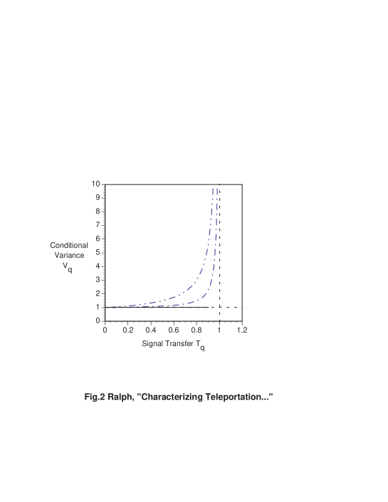
Figure 2: Performance of classical teleportation arrangement. Two quadrature signal transfer ($T_{q}=T_{s}^{+}+T_{s}^{-}$) is plotted versus two quadrataure conditional variance ($V_{q}=(V_{\rm cv}^{+}+V_{\rm cv}^{-})/2$) for $\lambda_{+}=-\lambda_{-}$ running from $0$ to $3.0$. Dashed lines indicate the classical limits. The double-dot-dashed line is for symmetric transmission of coherent state and the dot-dashed line is for a 90% squeezed state. The solid line is for asymmetric transmission of a coherent state.

These results are summarized for a coherent input state in Fig. 2 where $T_{q}$ versus $V_{q}$ is plotted as a function of increasing gain (we will refer to this as the $T-V$ graph. The dashed lines represent the limits set by purely classical transmission. The dash-double-dot line shows a symmetric scheme, i.e. one which detects and transmits information about both quadratures equally whilst the solid line is for an asymmetric scheme. With symmetric transmission it is only possible to reach the classical limits at the extrema of the gain. However, in the limit of high gain, asymmetric transmission approaches the point $T_{q}=V_{q}=1$. The region between the symmetric, coherent curve and the classical limits can also be accessed in a symmetric transmission scheme with an asymmetric input state such as a squeezed state. This is shown as the dot-dashed line in Fig. 2. However for no classical detection-transmission scheme or input state can one go below $V_{q}=1$ or (for a minimum uncertainty state) above $T_{q}=1$.

So what do these criteria tell us? The two quadrature transfer coefficient ($T_{q}$) describes the reliability with which two independent signal streams which have been encoded simultaneously on the conjugate quadratures, can be passed through the classical channel. A quantum channel can carry more information than can be reliably extracted from it. In principle all the information carried by a classical channel can be extracted, hence information must be lost in going from the quantum to the classical channel. If $T_{q}>1$ then the transmission channel can not be considered purely classical. The consequences of this with regard to the actual amount of information that can be transferred depends on the size and type of the encoded signals. From the point of view that the signals are states, $T_{q}$ could be considered a measure of the distinguishability of the input states on the output. Note again that $T_{q}=1$ is only a quantum limit for minimum uncertainty states.

The limit imposed by the two quadrature conditional variance ($V_{q}$) may be considered more fundamental. For two individual beams in any state the limit $V_{q}\geq 1$ cannot be exceeded, regardless of any common history. By individual we mean that independent measurements can be made on each beam. If $V_{q}<1$ then it implies that the input and output must be considered to be part of the same beam at the quantum level. This represents a neccessary condition for the transfer of any quantum correlations between the input and output. Such quantum correlations lead to the unique character of quantum information, hence the passing of this limit is very important. However most practical applications will also demand good signal to noise transfer.

III Quantum Teleportation

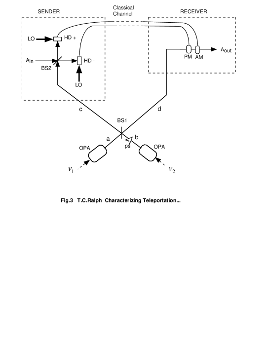
Figure 3: Schematic of quantum teleportation arrangement. Symbols as for Fig.1 plus; OPA:Optical parametric amplifier, ps:$\pi/2$ phase shift and BS1 and BS2 are 50:50 beamsplitters.

We now introduce a quantum channel and examine under what conditions the classical limits are exceeded. Consider the electro-optical arrangement that is shown in Fig. 3. It is similar to that employed by Furusawa et al Ref.[7]. The entanglement is provided by two coherently related amplitude squeezed sources from optical parametric amplifiers (OPA’s). These are mixed on a 50:50 beam splitter (BS1). The OPA’s are seeded with the coherent beams, $\hat{v}_{1}$ and $\hat{v}_{2}$, giving output beams

$$\hat{a} = \sqrt{H}\hat{v}_{1}-\sqrt{H-1}\hat{v}_{1}^{\dagger}$$

$$\hat{b} = \sqrt{H}\hat{v}_{2}-\sqrt{H-1}\hat{v}_{2}^{\dagger}$$ (20)

where $H$ is the parametric gain. They are combined with a $\pi/2$ phase shift giving rise to the output beams

$$\hat{c} = \sqrt{H}\hat{v}_{3}-\sqrt{H-1}\hat{v}_{4}^{\dagger}$$

$$\hat{d} = \sqrt{H}\hat{v}_{4}-\sqrt{H-1}\hat{v}_{3}^{\dagger}$$ (21)

where $\hat{v}_{3}={{1}\over{\sqrt{2}}}(\hat{v}_{1}+i\hat{v}_{2})$ and $\hat{v}_{4}={{1}\over{\sqrt{2}}}(\hat{v}_{1}-i\hat{v}_{2})$, are formally equivalent to independent coherent inputs. One of the outputs from the beamsplitter ($\hat{c}$) is sent to where we wish to measure the input signal. There it is mixed with the input signal beam on another 50:50 beamsplitter (BS2). The beams are mixed with local oscillators (LO) and homodyne detection is used to measure the phase quadrature of one beam and the amplitude quadrature of the other (represented schematically in Fig. 3). The photocurrents thus obtained are sent to amplitude and phase modulators situated in the other beam ($d$) coming from the mixed squeezed sources. Here we attempt to reconstruct the original beam. The specific set-up outlined above could be a convenient experimental realization when using bright beams. For dim input beams one could use squeezed vacua to create the entanglement and a Mach-Zender modulation scheme (see Fig.1(a)) for reconstruction. In general the required entanglement can be created by the mixing of any two coherently related squeezed beams, irrespective of the intensity or the quadrature of their squeezing, provided they are mixed with the correct phase relationship. The following results are not dependent on the specific scheme employed.

Following the approach of Ref. [22], the amplitude and phase noise spectra of the output field are found to be

$$V_{\rm out}^{\pm} = {1\over 2}\left|{\sqrt{\eta_{d}}+\lambda_{\pm}\sqrt{\eta_{c}\eta_{e}}}\right|^{2}V_{a}^{\pm}+{1\over 2}\left|{\sqrt{\eta_{d}}-\lambda_{\pm}\sqrt{\eta_{c}\eta_{e}}}\right|^{2}V_{b}^{\mp}$$ (22)

$$+\left|{\lambda_{\pm}}\right|^{2}\eta_{e}V_{\rm in}^{\pm}+(1-\eta_{d})+\lambda^{2}(1-\eta_{c}\eta_{e})$$

Here the amplitude (phase) spectra of beams $a$ and $b$ are given by $V_{a}^{+}=\sqrt{H}-\sqrt{H-1}$ ($V_{a}^{-}=\sqrt{H}+\sqrt{H-1}$) and $V_{b}^{+}=\sqrt{H}-\sqrt{H-1}$ ($V_{b}^{-}=\sqrt{H}+\sqrt{H-1}$) respectively. The transmission efficiencies of beams $\hat{c}$ and $\hat{d}$ are given by $\eta_{c}$ and $\eta_{d}$ respectively, whilst the sender’s detection efficiency is given by $\eta_{e}$. The cross coupling of the phase spectrum of beam $\hat{b}$ into the amplitude spectrum of the output is due to the $\pi/2$ phase shift. We assume initially no loss ($\eta_{c}=\eta_{d}=\eta_{e}=1$). Consider the situation if beams $\hat{b}$ and the signal are blocked so that just vacuum enters the empty ports of the beamsplitters. The set-up is then just a feedforward loop. Lam et al [22] have shown that the measurement penalty at the feedforward beamsplitter (BS1) can be completely canceled by correct choice of the electronic gain, allowing noiseless amplification of $V_{a}^{+}$ to be achieved. This cancellation can be seen from Eq. 22 with the electronic gain set to $\lambda_{+}=1$. The remaining penalty is due to the in-loop beamsplitter (BS2) which, here, is allowing us to detect both quadratures. But now suppose we inject our signal into the empty port of the in-loop beamsplitter. With $\lambda_{+}=1$ we find Eq. 22 reduces to

$$V_{\rm out}^{+}=2V_{a}^{+}+V_{\rm in}^{+}$$ (23)

and if beam $a$ is strongly amplitude squeezed such that $V_{a}^{+}<<1$ then

$$V_{\rm out}^{+}\simeq V_{\rm in}^{+}$$ (24)

Now consider the phase noise spectrum, Eq. 22. If we impose the same electronic gain condition on the fed-forward phase signal as we have for the amplitude signal we will get an output spectrum

$$V_{\rm out}^{-}=2V_{a}^{-}+V_{\rm in}^{-}$$ (25)

If beam $\hat{a}$ is strongly amplitude squeezed then the uncertainty principle requires $V_{a}^{-}>>1$ so this is not a useful arrangement. However if we perform negative rather than positive feedforward on our phase signal such that $\lambda_{-}=-1$ then we will cancel the phase noise of beam $\hat{a}$ and instead see the vacuum noise entering at the empty port of the feedforward beamsplitter. Finally by injecting beam $\hat{b}$ at this port we find

$$V_{\rm out}^{-}=2V_{b}^{+}+V_{\rm in}^{-}$$ (26)

Beam $\hat{b}$ can be made strongly amplitude squeezed without affecting Eq. 24 thus giving us

$$V_{\rm out}^{-}\simeq V_{\rm in}^{-}$$ (27)

Hence we have the remarkable result that we can satisfy both Eqs. 24 and 27 simultaneously even though the only direct connection between the input and output fields is classical; i.e. teleportation of our input field. More generally, the spectral variance at some arbitrary quadrature phase angle ($\theta$) is given by

$$V_{\rm out}^{\theta} = \left\langle{\left|{\delta A_{\rm out}^{\dagger}e^{+i\theta}+\delta A_{\rm out}e^{-i\theta}}\right|^{2}}\right\rangle$$ (28)

$$= V_{\rm in}^{\theta}+2\cos^{2}\theta\;V_{a}^{+}+2\sin^{2}\theta\;V_{b}^{+}$$

This form makes it clear that, provided beam $\hat{a}$ and beam $\hat{b}$ are both strongly amplitude squeezed, the input and output spectral variances will be approximately equal for any arbitrary quadrature angle (not just amplitude and phase). Note that, as for other teleportation schemes, no quantum limited information about the input field can be obtained from the classical channels. This is because it is “buried” by the large anti-squeezed fluctuations that are mixed with the input beam at the measurement site. The strong EPR correlations carried by the quantum channel enable this quantum information to be retrieved on the receiver beam.

It is clear that under the ideal conditions of no losses and very strong squeezing the best operating point is unity gain, i.e. $\lambda=1$ where $\lambda_{+}=-\lambda_{-}=\lambda$. However this is not so clear under non-ideal conditions. In Fig. 4 we plot $T_{q}$ versus $V_{q}$ for a coherent input as a function of feedforward gain for various values of squeezing. Notice that although a moderate value of squeezing allows either information transfer or the correlation to be superior to the classical channel limit, squeezing must be greater than 50% before both conditions can be met simultaneously. This limit remains valid for arbitrary input states as the point $T_{q}=V_{q}=1$ is the unity gain point for all input states when the squeezing is 50%.

We can learn a lot about the operation of the teleporter by looking at the turning points of the $T-V$ graph. A maximum in $T_{q}$ occurs for gain $\lambda_{G}=(V_{a}+1)/(V_{a}-1)$. At this point the output is simply an amplified version of the input, i.e.

$$\delta\hat{A}_{{\rm out},G}=\lambda_{G}\delta\hat{A}_{\rm in}+\sqrt{\lambda_{G}^{2}-1}\delta\hat{v}_{3}^{\dagger}$$ (29)

where we have subtracted off the classical coherent amplitude of the field as per Eq.1. On the other hand a minimum in $V_{q}$ occurs for gain $\lambda_{\eta}=(V_{a}-1)/(V_{a}+1)=1/\lambda_{G}$. At this point the output is simply the attenuated version of the input

$$\delta\hat{A}_{{\rm out},\eta}=\lambda_{\eta}\delta\hat{A}_{\rm in}+\sqrt{1-\lambda_{\eta}^{2}}\delta\hat{v}_{4}$$ (30)

The other point of interest is unity gain as this is approximately the point of maximum fidelity [7]. Here the output is formally equivalent to equal amounts of amplification followed by attenuation being applied to the input state and is given by

$$\delta\hat{A}_{{\rm out},F}=\delta\hat{A}_{\rm in}+\sqrt{1-\lambda_{\eta}^{2}}(\delta\hat{v}_{4}^{\dagger}+\delta\hat{v}_{3})$$ (31)

In the limit of no squeezing, $V_{a}\to 1$, we go to the classical limit where the minimum in $V_{q}$ occurs for $\lambda\to 0$ with the output looking like a very strongly attenuated version of the input, and the maximum in $T_{q}$ occurs for $\lambda\to\infty$ with the output looking like a very strongly amplified version of the input. The output at the unity gain point is a very strongly amplifed, then equally strongly attenuated version of the input, effectively a classical channel [23]. In the opposite limit of very strong squeezing, $V_{a}\to 0$, all three points converge on unity gain with the effective attenuation and amplification also tending to unity, i.e. the output tends to a perfect copy of the input.

As might be expected these ideal results are degraded by loss. The effect of loss on the entangled beams is asymmetric, i.e. loss in beam $\hat{c}$ is more detrimental to $V_{q}$ than $T_{q}$, whilst loss in beam $\hat{d}$ is more detrimental to $T_{q}$ than $V_{q}$. The system is most vulnerable to detection losses. Detection losses of greater than 50% prevent any crossing of the quantum limits. Fortunately, in recent years losses in homodyne detection systems have been reduced to under 10% [24]. If beams $\hat{a}$ and $\hat{b}$ are not minimum uncertainty squeezed states the results will also be degraded except at the unity gain point where exact cancellation of the conjugate quadrature occurs.

IV Discussion

The best gain to use in a particular teleportation experiment clearly depends on the amount of squeezing available and the characteristics of the input field you most wish to preserve. For example if the input was in a squeezed state and one wished the output to still exhibit non-classical statistics you would operate at the point $\lambda_{\eta}$. The output will always exhibit some squeezing at this point (in the absence of loss), though possibly very small if $\lambda_{\eta}$ is small. In fact if the squeezing on the input is very large, squeezing will be seen on the output over all gains for which $V_{q}<1$ (irrespective of loss), but never outside this range. For lower levels of input squeezing the range of output squeezing will be reduced. Hence this condition can be regarded as neccessary but not sufficient for the teleportation of non-classical statistics. We have recently shown that very similar behaviour happens in the teleportation of non-local correlations [12]. One can use a two polarization mode generalization of the continuous variable technique to teleport one of a non-locally entangled pair of photons. By examining the coincidence detection rates between the teleported and unteleported pairs after polarization filtering it can be determined if non-local correlations are still present. For the case of no loss it is found that by sitting at the point $\lambda_{\eta}$ a maximal violation of the Clauser-Horne inequality [25] is always achieved, regardless of the amount of squeezing in the entangled states. This occurs because at the point $\lambda_{\eta}$ the output is a pure attenuation of the input and nonlocal measures which use coincidence counting are insensitive to attenuation. Of course any information carried will be strongly degraded if $\lambda_{\eta}$ is too small.

We can now understand the difference in the accomplishments of the photon number and continuous variable experiments. In the photon number experiment of Boumeester et al [3] the operating point was effectively a gain of $\lambda_{\eta}$, which was rather small because a weakly pumped (thus not very squeezed) type II OPO was used as the source of entanglement. This enabled non-local coincidence correlations to be shown, implying the limit $V_{q}=1$ had been broken, but with very low coincidence count rates such that effectively $T_{q}<<1$. Arguing from analogy with the results of Ref. [12] the position of this experiment on the $T-V$ graph might be approximated by the cross on Fig.4. Being a long way from unity gain, the average fidelity in this experiment was low. On the other hand in the continuous variable experiment of Furukawa et al [7] the fidelity was maximized by operating at the unity gain point. The position of this experiment on the $T-V$ graph is indicated by the star on Fig.4 which lies under the coherent state limit indicated by the solid line. By picking the optimum compromise between signal and correlation preservation the greatest similarity between input and output states is obtained. However because less than 50% squeezing was available neither their signal transfer nor their correlation broke the quantum limits individually. We believe that for any useful application of teleportation to quantum information manipulation it will be neccessary for the teleporter to operate in the lower-right hand quadrant of the $T-V$ graph.

Discussions with S L Braunstein, H J Kimble and many others helped to clarify some of the issues explored in this paper. This work was supported by the Australian Research Council.

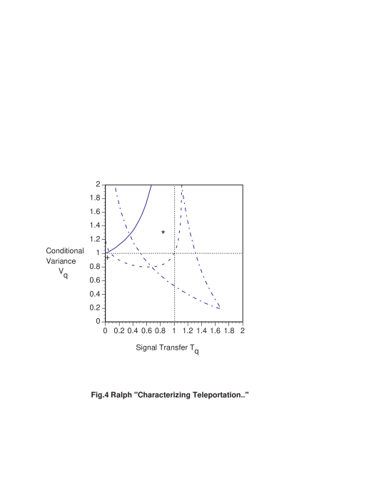
Figure 4: Performance of quantum teleportation arrangement with a coherent input. The solid line is with no squeezing, the dashed line is 50% squeezing and the dot-dashed line is for 90% squeezing. The dotted lines are the classical limits for any minimum uncertainty input.

References

- [1] A Einstein, B Podolsky and N Rosen, Phys. Rev. 47, 777 (1935).
- [2] C H Bennett, G Brassard, C Crepeau, R Jozsa, A Peres and W K Wootters, Phys Rev Lett 70, 1895 (1993).
- [3] D Boumeester, J-W Pan, K Mattle, M Eibl, H Weinfurter and A Zeilinger, Nature (London) 390, 575 (1997).
- [4] D Boschi, S Branca, F De Martini, L Hardy and S Popescu, Phys Rev Lett 80, 1121 (1998).
- [5] L Vaidman, Phys Rev A 49, 1473 (1994).
- [6] S L Braunstein and H J Kimble, Phys Rev Lett 80, 869 (1998).
- [7] A Furusawa, J L Sorensen, S L Braunstein, C A Fuchs, H J Kimble and E S Polzik, Science, 282, 706 (1998).
- [8] Z Y Ou, S F Pereira, H J Kimble, and K C Peng, Phys Rev Lett 68, 3663 (1992).
- [9] G Brassard, S L Braunstein and R Cleve, Physica D 120, 43 (1998).
- [10] C H Bennett, Phys.Today 48, 24 October (1995).
- [11] S L Braunstein, Nature 394, 47 (1998).
- [12] “Teleporting Non-locality with Continuous Variables”, R E S Polkinghorne and T C Ralph, submitted to Phys Rev Lett (1998).
- [13] B Schumacher, Phys Rev A 51, 2738 (1995).
- [14] G Breitenbach, S Schiller and J Mlynek, Nature 387, 471 (1997).
- [15] T C Ralph and P K Lam, Phys Rev Lett 81, 5668 (1998).
- [16] J-Ph Poizat, J-F Roch and P Grangier, Ann Phys Fr. 19, 265 (1994).
- [17] H P Yuen and J H Shapiro, IEEE Trans. IT 26, 78 (1980).
- [18] Y Yamamoto and H A Haus, Rev Mod Phys 58, 1001 (1986).
- [19] E Arthurs and M S Goodman, Phys Rev Lett 60, 2447 (1988).
- [20] H M Wiseman, M S Taubman and H-A Bachor, Phys Rev A 51, 3227 (1995).
- [21] M J Holland, M J Collett, D F Walls and M D Levenson, Phys Rev A 42, 2995 (1990).
- [22] P K Lam, T C Ralph, E H Huntington and H-A Bachor, Phys Rev Lett 79, 1471 (1997).
- [23] “All optical teleportation”, T C Ralph, Opt.Lett, in press (1999).
- [24] P K Lam et al, this issue (1999).
- [25] J F Clauser and M A Horne, Phys Rev D 10, 526 (1974).