A Method of Areas for Manipulating the Entanglement Properties of One Copy of a Two-Particle Pure Entangled State

Abstract

We consider the problem of how to manipulate the entanglement properties of a general two-particle pure state, shared between Alice and Bob, by using only local operations at each end and classical communication between Alice and Bob. A method is developed in which this type of problem is found to be equivalent to a problem involving the cutting and pasting of certain shapes along with certain colouring problems. We consider two problems. Firstly, we find the most general way of manipulating the state to obtain maximally entangled states. After such a manipulation the entangled states $|11\rangle+|22\rangle+\dots+|mm\rangle$ are obtained with probability $p_{m}$. We obtain an expression for the optimal average entanglement obtainable. Also, some results of Lo and Popescu pertaining to this problem are given simple geometric proofs. Secondly, we consider how to manipulate one two-particle entangled state $|\psi\rangle$ to another $|\psi^{\prime}\rangle$ with certainty. We derive Nielsen’s theorem (which states a necessary and sufficient condition for this to be possible) using the method of areas.

1 Introduction

Quantum entanglement has many applications including quantum teleportation [1], quantum cryptography [2], and quantum communication [3]. This has led people to regard entanglement as a resource. However, entanglement can exist in different forms and so it is useful to know how it can be manipulated from one form to another. In this paper the problem of manipulating a general pure two-particle entangled state in order to obtain maximally entangled states will be considered. We will also consider the problem of how to manipulate one general pure two-particle entangled state to another. Alice and Bob are allowed to do whatever they want locally and they are allowed to communicate classically with one another. They are not allowed to exchange quantum states. This type of situation has already been much discussed in the literature. The problem of how to optimally manipulate a large number, $N$, of copies of a general pure two-particle entangled states into maximally entangled states by local means has been completely solved in the asymptotic limit $N\rightarrow\infty$ [4]. However, the perhaps more basic problem of how to manipulate a single copy of a general pure two-particle state into maximally entangled states has not been so extensively discussed. The most significant work on this is by Lo and Popescu [5] who prove certain bounds relating to this problem. However their proofs, while being extraordinarily ingenious, are rather difficult to follow. The method developed in this paper, which completely solves the problem, involves the cutting and pasting of areas along with a colouring problem. Once the basic methods have been put in place, it is very easy to picture what is happening. This method is used to find the maximum obtainable average entanglement and to derive a formula of Lo and Popescu which gives the maximum probability of obtaining a given maximally entangled state.

A related problem is how to transform one pure two-particle entangled state to another, and to establish which states will transform to one another in this way. Nielsen [6] has completely solved this problem. However his proof of his theorem uses some unfamiliar mathematics. An alternative reasonably simple proof of Nielsen’s theorem is given here which, again, involves cutting and pasting of areas along with a certain colouring problem.

2 Obtaining maximally entangled states

2.1 Introduction

The most general pure two-particle state can be written in the Schmidt form

$$|\psi\rangle=\sum_{i=1}^{I}\sqrt{\lambda_{i}}|i\rangle_{A}|i\rangle_{B}$$ (1)

where we choose $\lambda_{i}\geq\lambda_{i+1}$ and where the states $|i\rangle_{A,B}$ are orthonormal. We want to manipulate this state in order to obtain states which are of the form

$$|\varphi_{m}\rangle={1\over\sqrt{m}}\sum_{k=1}^{m}|k\rangle_{A}|k\rangle_{B}$$ (2)

We will call this state an $m$-state. An $m$-state is equivalent to $\log_{2}m$ copies of 2-states [4]. After the process is completed we should have a certain $m$-state with a certain probability $p_{m}$. Particle A goes to Alice and particle B goes to Bob. Alice and Bob are allowed to perform whatever operations they want locally and also they communicate classically with each other. This can happen in the following way. Alice performs a measurement and communicates the result to Bob who then performs a measurement which depends on the result of Alice’s measurement, and then Bob communicates his result back to Alice and she makes another measurement, and so on back and forth. This is most general way in which Alice and Bob can manipulate their state without actually exchanging quantum states in the process. Whatever measure of entanglement we employ, the amount of entanglement should not increase during such a process. Lo and Popescu show that, for the very special case of a two-particle pure state, this process is equivalent to one in which Alice makes one measurement and communicates the result to Bob who then may perform a unitary evolution operation on his particles. The reason for this significant simplification is that, due to the Schmidt decomposition, any operation by Bob is equivalent, so far as the resulting form of the state is concerned, to some operation by Alice. Hence, Alice can simply do everything herself in one go and then communicate the final result to Bob. The most general measurement Alice can make is a POVM. This is equivalent to Alice introducing an ancilla, $S$, performing a general unitary evolution on particle $A$ and the ancilla $S$, and then making a projective measurement on the ancilla. Let us imagine that the ancilla has a basis set of states $|l\rangle_{S}$. Since we allow completely general evolution of $A+S$ we can assume, without loss of generality, that the final measurement projects onto subspaces spanned by the states $|l\rangle_{S}$. Furthermore, it is shown in the appendix that there is no advantage to be had by performing a non-maximal (i.e. degenerate) measurement and so we can assume that this measurement is maximal and projects onto the operators $|l\rangle_{S}\langle l|$. For each outcome, $l$, the two particles $A$ and $B$ should be projected into an $m$-state $|\varphi_{m_{l}}\rangle^{l}$ where

$$|\varphi_{m_{l}}\rangle^{l}={1\over\sqrt{m_{l}}}\sum_{k=1}^{m_{l}}|k\rangle_{A}|k\rangle_{B}^{l}$$ (3)

The superscript $l$ is included since we do not require that the Schmidt vectors satisfy $|k\rangle_{B}^{l}=|k\rangle_{B}^{l^{\prime}}$ for $l\not=l^{\prime}$. After Alice has communicated the result, $l$, of the measurement to Bob, Bob could rotate these vectors into the same standard form for all $l$ (thus removing the need for the superscript at this stage), but this is not important. It is enough that Alice and Bob know what $l$ is so they know what state they have. We do not require a superscript $l$ on the $|k\rangle_{A}$ states since, as explained below, Alice can rotate her Schmidt vectors to standard form as part of the overall unitary transformation she performs. Just before Alice makes her measurement projecting onto $|l\rangle_{S}$ the state of the system will be

$$|\Psi_{\rm target}\rangle=\sum_{l}\sqrt{\mu_{l}}|l\rangle_{S}|\varphi_{m_{l}}\rangle^{l}$$ (4)

where the coefficients $\sqrt{\mu_{l}}$ can be taken to be real since any phases can be absorbed into appropriately redefined $|l\rangle_{S}$. Note that if, at this stage, the $|i\rangle_{A}$ states had a superscript $l$ then they could be rotated into standard form by applying a series of controlled unitary operations, $\hat{U}_{l}$, to $A$ where the control is the $|l\rangle_{S}$ state. At this stage Alice has not done anything which is irreversible. Having completed her local manipulations Alice will perform a maximal projective measurement. It follows from the result of Lo and Popescu that manipulating the state into the form (4) and then measuring onto the $|l\rangle_{S}$ basis is equivalent to the most general procedure for manipulating the two particles by local means to $m$-states. We will use equation (4) later when we come to show that the method developed in the next section is equivalent to the most general method.

2.2 How to obtain maximally entangled states

Now consider the initial state $|\psi\rangle$ given in equation (1). We will introduce an ancilla, $R$, in the state $|1\rangle_{R}$. This ancilla has basis states $|n\rangle_{R}$ where $n=1,2,\dots N$. We will take $N$ to be very large and will want to consider the case where $N$ tends to infinity. We define the integers $N_{i}=N\lambda_{i}$ where, for the moment, we are taking the $\lambda_{i}$ to be rational numbers so the integers $N_{i}$ can be found with $N$ finite. This constraint can be relaxed when $N$ tends to infinity. The initial state of $RAB$ is $|1\rangle_{R}|\psi\rangle$. Alice now evolves $R+A$ using the following transformations.

$$|1\rangle_{R}|i\rangle_{A}\rightarrow{1\over\sqrt{N_{i}}}(\sum_{n=1}^{N_{i}}|n\rangle_{R})|i\rangle_{A}$$ (5)

The fact that these transformations evolve orthogonal states to orthogonal states ensures that they can be implemented by unitary evolution. Under these transformations the state $|1\rangle_{R}|\psi\rangle$ evolves to

$$|\Psi_{\rm start}\rangle={1\over\sqrt{N}}\sum_{i}\sum_{n=1}^{N_{i}}|n\rangle_{R}|i\rangle_{A}|i\rangle_{B}$$ (6)

which we will call the start state. We see that each of the $N$ terms in this superposition has the same amplitude. Each of these terms will be represented by a rectangular element width 1 and height $1/N$. The area of the element is $1/N$ and equal to the probability associated with the corresponding term in (6). Each element can be labelled by $(n,i)$ corresponding to the term $|n\rangle_{R}|i\rangle_{A}|j\rangle_{B}$ (initially $i=j$ but after Alice has performed operations on her particles this will not necessarily be the case for every term). The elements are then arranged on a graph where elements having the same $n$ are placed in the same row and elements having the same $i$ are placed in the same column. The resulting graph looks like a series of steps as shown in Fig. 1.

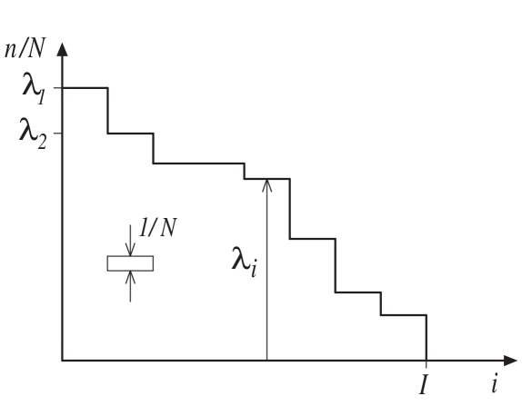
Figure 1: The start state can be plotted on a graph. Such a graph is called an area diagram. This area diagram has step structure in which the steps go down towards the right.

We will call this the area diagram. The total area under the steps is 1 corresponding to the total probability. On the vertical axis $n/N$ is plotted. On the horizontal axis the $i$ which appears in $|i\rangle_{A}$ is plotted. For small $n$ every $i$ position will be filled. However, because of the form of the state (6), once $n$ gets bigger than $N_{I}$ there will no longer be any $|I\rangle_{A}|I\rangle_{B}$ terms. This is the reason for the step at $n=N_{I}$. There will be further steps at each $n=N_{i}$. The height of the rightmost step is $N_{I}/N=\lambda_{I}$. Subsequent steps will be at heights $\lambda_{i}$ as shown in Fig. 1. If a projective measurement were to be performed on $R$ at this stage then, corresponding to each outcome $n$, the state of $A+B$ would be projected onto an $m$-state where $m$ is equal to the number of elements in the $n$th row on the area diagram. This will give a distribution of $m$-states with probabilities which are equal to the large horizontal rectangular areas of width $m$ and height $\lambda_{m}-\lambda_{m+1}$ formed by extending the horizontal parts of the step back to the vertical axis. However, the area in the diagram can be moved around by Alice in a way to be described below by performing local unitary operations. When this is followed by a projective measurement on $R$ different distributions of $m$-states can be realised.

The terms $|n\rangle_{R}|i\rangle_{A}|j\rangle_{B}$ and $|n^{\prime}\rangle_{R}|i^{\prime}\rangle_{A}|j^{\prime}\rangle_{B}$ are bi-orthogonal iff ${}_{R}\langle n|n^{\prime}\rangle_{R}{}_{A}\langle i|i^{\prime}\rangle_{A}=0$ (orthogonal at Alice’s end) and ${}_{B}\langle j|j^{\prime}\rangle_{B}=0$ (orthogonal at Bob’s end). If two terms are only orthogonal at either Alice’s end or at Bob’s end then they are mono-orthogonal. In the area diagram we will impose the constraint that all elements in a row, that is for a given $n$, correspond to terms which are bi-orthogonal. This ensures that when we perform a projective measurement onto $R$ the resulting state will be an $m$-state.

We will colour all the elements which correspond to terms which are mono-orthogonal to one another a given colour. Elements corresponding to terms which are bi-orthogonal will be coloured with different colours. Thus, initially, all the elements in a given column are the same colour and every column is coloured a different colour to every other column. When area is moved around the constraint that terms corresponding to elements in a row be bi-orthogonal means that all elements in any given row must be different colours.

The method of areas to be developed here involves moving area elements around in such a way that there is a net movement of area up and to the left. We will see that it is possible to have a net movement of area up the area diagram but not down the diagram. This means that the net movement of area across any horizontal line drawn on the diagram must be up. The basic unitary operation, $U(n,i\leftrightarrow n^{\prime},i^{\prime})$, employed by Alice is defined by the transformation equations

$$|n\rangle_{R}|i\rangle_{A}\rightarrow|n^{\prime}\rangle_{R}|i^{\prime}\rangle_{A}$$ (7)

$$|n^{\prime}\rangle_{R}|i^{\prime}\rangle_{A}\rightarrow|n\rangle_{R}|i\rangle_{A}$$ (8)

with no change for all other $|n^{\prime\prime}\rangle_{R}|i^{\prime\prime}\rangle_{A}$. We will call this the swap operation. The effect of this operation is to move elements around on the area diagram. If there are elements at both the $(n,i)$ and $(n^{\prime},i^{\prime})$ positions then they will have their positions swapped. If, there is only an element at one of the two positions then it will be moved to the other position while the original position will become vacant. These moves will not effect Bob’s part of the state. If two terms are bi-(mono)-orthogonal before the swap operation is applied to one or both of them then they will be bi-(mono)-orthogonal afterwards. In other words, the swap operation does not change the colour of the elements. Initially, as stated above, all elements in the same row are different colours and elements in the same column are the same colour. In moving elements of area around we impose only the constraint that, at the end of the process, all elements in a row are different colours. Although elements in any given column start off being the same colour, we do not demand that this is true at the end of the process. We can move a large number of elements at once. In the limit as $N\rightarrow\infty$ the elements will become infinitesimal in height. Hence, in this limit, we can make horizontal cuts anywhere. We can make vertical cuts along the edges of the columns. The area can be cut up into smaller pieces and then pieces can be moved around and pasted into new positions. It is possible to move area around like this in any way we want by repeated applications of the swap operation. The empty space above the steps can be used as a clipboard for the temporary storage of pieces of area to facilitate the rearrangement of area if required.

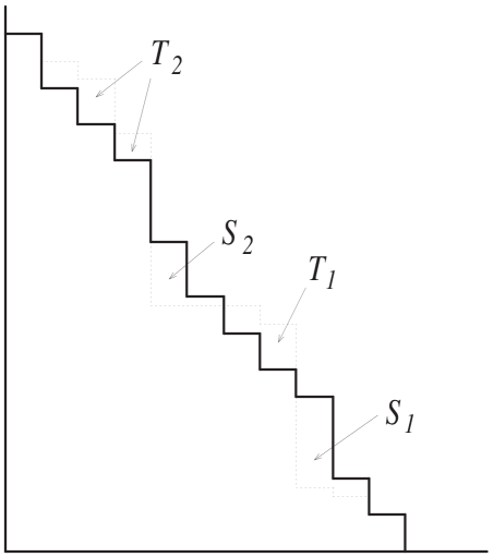
Figure 2: Area is transferred up the area diagram to go from the start steps shown by the bold line to the target steps shown by the dashed line. The total area transferred up is $S=T$

In Fig. 2 the original step structure is shown by a full line. A new step structure is shown by a dashed line. We will impose the constraint (to be justified later) that the new step structure consists of steps which, like the original steps, go across and down (but never up) towards the right. The area $S=\sum S_{r}$ which will be cut away from some parts of the steps is equal to the area $T=\sum T_{r}$ which will be added to other parts of the steps. Each of these areas consist of $R$ smaller disjoint parts labelled by $r$ going up the diagram. Note, area $T_{r}$ lies between area $S_{r}$ an $S_{r+1}$. Note also that the areas $S_{r}$ and $T_{r}$ can themselves be made up of disjoint parts. The constraint that there is no net movement of area downwards means that $\sum_{r=1}^{r^{\prime}}T_{r}\leq\sum_{r=1}^{r^{\prime}}S_{r}$ for all $r^{\prime}$. The original steps are of height $\lambda_{i}$. Let the new steps be of height $\lambda^{\prime}_{i}$. Since the columns are of unit width, these lengths are numerically equal to the areas of the columns, and hence the constraint that area is moved only to the left is equivalent to the set of constraints

$$\sum_{i=p}^{I}\lambda^{\prime}_{i}\leq\sum_{i=p}^{I}\lambda_{i}$$ (9)

for all $r=1$ to $I$ with equality holding when $r=1$.

We could simply move the area $S$ to the area $T$ element by element by applying the swap operator. However, if we did this it is likely that elements corresponding to mono-orthogonal terms would end up in the same row. If we can redistribute the area so that it corresponds to the new step structure but without there being any elements of the same colour in the same row then we will have realised another distribution of $m$-states. This is because Alice could then perform a projective measurement on $R$ and corresponding to each outcome, $n$, will be a $m$-state and these $m$-states will clearly have a different distribution. The probability of a given $m$ state is equal to the area of the horizontal rectangle formed by projecting leftwards the top and bottom of the step at position $m$. This rectangle has width $m$ and height $\lambda^{\prime}_{m}-\lambda^{\prime}_{m+1}$. Hence, for the new area diagram, the probability of getting an $m$ state is

$$p_{m}=(\lambda^{\prime}_{m}-\lambda^{\prime}_{m+1})m$$ (10)

We will show firstly that this colouring problem can be solved and secondly that the process described here is general in the sense that any distribution of $m$-states which can be achieved by local means can be achieved by this method. Hence, equations (9) and (10) define the possible distributions of $m$-states that can be obtained.

The solution to the colouring problem will be explained by reference to the example shown in Fig. 3.

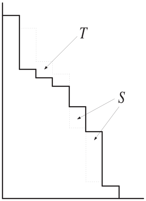
Figure 3: This figure shows the start steps (bold line) and the target steps(dashed line) of the recolouring problem discussed in the text.

This example has $R=1$ (since all of $T$ is above all of $S$). However, it will be clear that the method works for the general case. We start by taking the rightmost column in the area $S$. This is area $A$ in Fig 4(a). This area is then swapped into the rightmost column of the area $T$ so that point $a$ coincides with point $a^{\prime}$ as shown in Fig. 4(b).

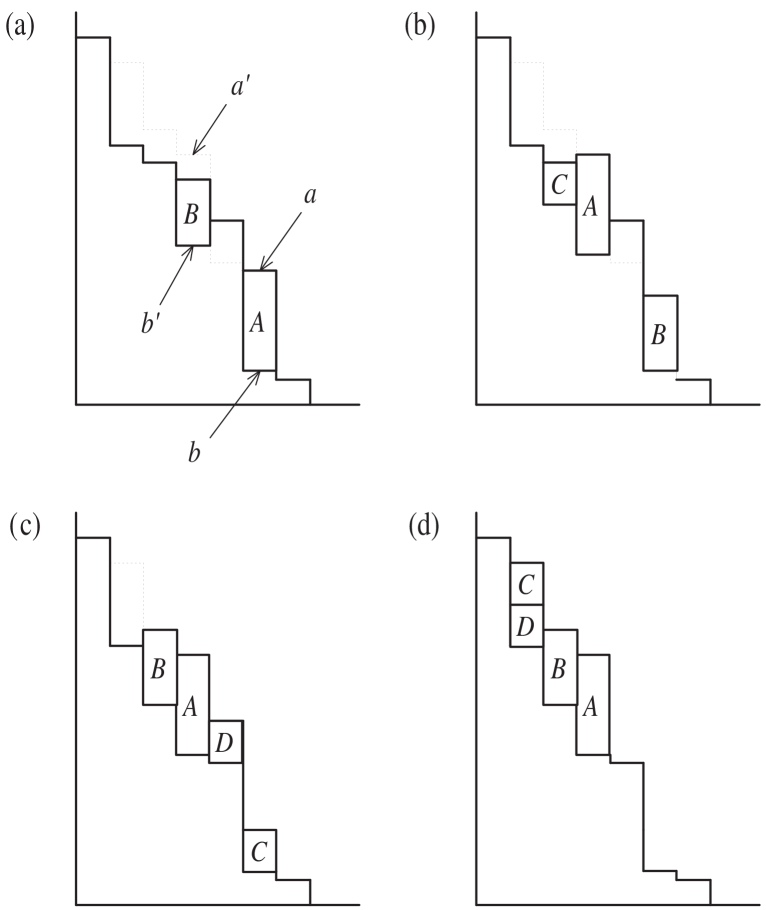
Figure 4: This figure shows the recolouring procedure described in the text. After the recolouring, no colour is in more than one place across any given row.

However, it may be too long to all fit in to the right most column of area $T$ (as is indeed the case in our example), and hence it will displace some of the area in the column below this, marked as area $B$ in Fig. 4(a). Because of the nature of the swapping operation, this area $B$ will be moved to the old position of $A$ so that point $b$ coincides with point $b^{\prime}$ as shown in Fig. 4(b). Area $A$ is now in its final position. Let us imagine that the column from which area $A$ was taken was coloured red. This red colour will now be divided between what is left of the original column and the area $A$ in its new position. Since the steps go up towards the left, it is impossible to have red at more than one position in any given row. The rightmost column of $T$ is now filled so we start on the next rightmost column. We swap area $B$ into position in the next rightmost column of area $T$. Again, this could be too long. In our example it is too long and projects into the column below into the area marked $C$. Hence $C$ will be moved to where $B$ was. This takes us to the situation shown in Fig. 4(c). Now we move area $C$ into position in the next rightmost column of area $T$. This could again be too long and project into the column below, but in this example this is not the case. Rather, area $C$ is too short leaving a gap. Hence no area is moved back to the rightmost column of $S$ and this means we have finally dispensed with the net effect of moving the area from this rightmost column of $S$. Now we select the next rightmost column of $S$. In our example this area is marked $D$ in Fig. 4(c). This area is now moved up following the same procedure. Thus, we move $D$ into position as high as possible in the rightmost column of $T$ which has not yet been filled. This places it below area $C$. It could be the case that $C$ is too long and projects into the column below in which case some area would be swapped back and we would have to continue as before. However, in our particular example area $D$ fits in below $C$ and the recolouring is finally completed as shown in Fig. 4(d). This method can be applied to any recolouring problem of this nature. The general method is that area is swapped from the rightmost non-empty column of $S$ to as high a position as possible in the rightmost non-full column of $T$. We note that a given colour can end up in, at most, two different columns and that any colour moved from a column will always end up higher than its original position. This means that it is impossible for two elements of area which started in the same column (having the same colour) to end up in the same row. Hence, the colouring problem has been solved.

2.3 Proof that this is most general method

Having shown that it is possible to have a net movement of area up the area diagram in any general way which is consistent with maintaining the step structure, we will now show that this corresponds to the most general way of manipulating entanglement to produce $m$-states in the sense that any distribution of $m$-states which can be achieved by local operations classical communication can be achieved by this method. The idea of this proof will be to show that the target state (just before Alice measures on to the ancilla) can be put into a certain form which is inconsistent with any movement of area downwards.

We have already established that the most general final state just before Alice makes her measurement (we call this the target state) is the state given in (4). If we write $\nu_{l}=\mu_{l}/m_{l}$ then (4) becomes

$$|\Psi_{\rm target}\rangle=\sum_{l}\sum_{k=1}^{m_{l}}\sqrt{\nu_{l}}|l\rangle_{S}|k\rangle_{A}|k\rangle_{B}^{l}$$ (11)

We can consider further unitary transformations by Alice on this state to put it into a form in which every term has the same amplitude. Let the dimension of the ancilla $S$ be $M$ and define $M_{l}=M\nu_{l}$ (again we will let $M\rightarrow\infty$) and let Alice perform the following transformations on (4):

$$|l\rangle_{S}\rightarrow{1\over\sqrt{M_{l}}}\sum_{n\in W_{l}}|n\rangle_{S}$$ (12)

where $W_{l}$ is the set of $M_{l}$ integers from $(\sum_{r=0}^{l-1}M_{r})+1$ to $\sum_{r=0}^{l}M_{r}$ (we put $M_{0}=0$). Under this transformation (4) becomes

$$|\Psi^{\prime}_{\rm target}\rangle={1\over\sqrt{M}}\sum_{l}\sum_{k=1}^{m_{l}}\sum_{n\in W_{l}}|n\rangle_{S}|k\rangle_{A}|k\rangle_{B}^{l}$$ (13)

Every term in this state has the same amplitude. In arriving at this state from the previous target state (4,11) we have done nothing that is irreversible. Furthermore, if we measure onto the $|n\rangle_{S}$ basis we are just as likely to get a given $m$-state as with the previous target state. Hence, we can regard this as our new target state. Any method by which $m$-states can be obtained is equivalent to manipulating the state into the form (13).

If we project onto $|n\rangle_{S}$ we will obtain an $m_{n}$-state where $m_{n}$ can be read off from (13). We can relabel the $n$’s such that $m_{n+1}\leq m_{n}$. Thus, we can impose the following:

Constraint A

If outcome $n$ corresponds to a $m_{n}$-state then, without loss of generality, we can impose the constraint that $m_{n+1}\leq m_{n}$.

By examining (13) we can see that there is a second constraint that can be imposed on the form of the final target state.

Constraint B

For the target state we can, without any loss of generality, impose the constraint that

$$|{}_{B}\langle\theta|{}_{S}\langle n|\Psi^{\prime}_{\rm target}\rangle|^{2}\leq{1\over M}$$ (14)

where $|\theta\rangle_{B}$ is any normalised state for system $B$ since this is true of equation (13).

We can identify the ancilla $S$ with the ancilla $R$ introduced earlier. Hence, $S\equiv R$ and $M=N$. Now consider the state (1). Since Alice’s operations do not effect Bob’s system we see that we have the following constraint:

Constraint C

While the state $|\Psi\rangle$ is being manipulated by local unitary operations by Alice, we will always have

$$|{}_{B}\langle j|\Psi\rangle|^{2}=\lambda_{j}={N_{i}\over N}$$ (15)

for all $j$.

Since (6) is related to (1) by reversible operations, we can take (6), which corresponds to an area diagram, as our starting point. We will now see that area cannot be moved down in the area diagram. For the purposes of this proof consider a change in the way the area diagram is plotted such that the $j$ in $|j\rangle_{B}$ (rather than the $i$ in $|i\rangle_{A}$) is plotted on the horizontal axis. This will simply have the effect of redistributing elements horizontally but not vertically since $n/N$ is still plotted on the vertical axis. We label elements in this modified area diagram by $\{n,j\}$. Constraint C implies that the column corresponding to a given $j$ on this modified area diagram will always have the same area. This is because Alice’s actions cannot effect the total area (or probability) associated with column $j$. However, Alice can change the $n$ value associated with area elements and hence she can move area in column $j$ up and down. It is possible that she can bring about a net movement of area (or probability) down in this column. This would lead to the area being compressed into a smaller space than it would “naturally” fit. Any net movement of area downwards, whether on the $\{n,j\}$ picture or the $(n,i)$ picture would correspond to this happening in at least one $j$ column. This is exactly what we want to rule out. We will now see that any such net movement downwards will violate constraint $B$ (which we were free to impose on the target state).

If, at some stage, the state has been manipulated to the state $|\Psi\rangle$ then the area of the $\{n,j\}$ element will be $A_{nj}=|{}_{B}\langle j|{}_{S}\langle n|\Psi\rangle|^{2}$. Initially, for the start state $|\Psi_{\rm start}\rangle$ in (6), we have

$$\sum_{n=1}^{n^{\prime}}A_{nj}^{\rm start}={n^{\prime}\over N}$$ (16)

for all $n^{\prime}\leq N_{i}$. However, if there is a net movement of area down the area diagram with respect to the horizontal line $n=n^{\prime}$ then, since the total area in a given column is constant (by constraint C), this net movement of area downwards must happen in at least one column of the modified area diagram. Hence, for at least one value of $j$, we must have

$$\sum_{n=1}^{n^{\prime}\leq N_{i}}A_{nj}^{\rm target}>{n^{\prime}\over N}$$ (17)

However, since $M=N$, equation (14) implies

$$\sum_{n=1}^{n^{\prime}\leq N_{i}}A_{nj}^{\rm target}\leq{n^{\prime}\over N}$$ (18)

The contradiction between (17) and (18) proves that a net movement of area downwards is not possible on the modified area diagram and hence neither is it possible on the unmodified area diagram. Note that this proof goes through for any sort of operations by Alice and in particular it does not assume that the only operations Alice can make are the swap operations defined in (7).

To complete the proof that the manipulations described earlier are equivalent to the most general way of manipulating the state to obtain $m$-states we note the following.

(i) The target state (13) can be represented on an area diagram in which $n/N$ (where $N=M$) is on the vertical axis and $m_{n}$ is plotted on the horizontal axis. Since $m_{n}$ is an integer and since we can impose constraint A without loss of generality, this area diagram will have a step structure (in which the steps of integer width go down towards the right).

(ii) The initial state can be taken to be the start state $|\Psi_{\rm start}\rangle$ given in (6) and this can be represented by an area diagram with the step structure.

(iii) The total area of both these diagrams is 1. Therefore the most general way of manipulating the start state into $m$-states corresponds to going from one area diagram with the step structure to another with the step structure in a way consistent with the constraint that there is no net movement of area downwards.

(iv) The method, employing the swap operator, discussed previously can be used to go from one step structure to another in any way that is consistent with there being no net downward movement of area. Hence, it is equivalent to the most general method.

2.4 Getting the highest possible average

If we are only interested in the average amount of entanglement in the form of maximally entangled states we can obtain, this being equal to $E=\sum_{m}p_{m}\log_{2}m$, then it turns out that any movement of area will decrease this average. Hence this average has a maximum given by the original area diagram

$$E^{\max}=\sum_{m}(\lambda_{m}-\lambda_{m+1})m\log_{2}m$$ (19)

To see that any movement of area will decrease this average, consider moving one element on the area diagram (with area equal to ${1\over N}$) from the end of row $A$ which has original width $m_{A}$, to the end of row $B$ which has original width $m_{B}$. Since we can only move area to the left we require that $m_{B}+1<m_{A}$ (if $m_{B}+1=m_{A}$ then the rows will simply have interchanged their lengths and hence there will be no change in the distribution of $m$-states). The original contribution of these two rows to $E$ will be

$$\Delta E_{\rm initial}={m_{A}\over N}\log_{2}m_{A}+{m_{B}\over N}\log_{2}m_{B}$$ (20)

The contribution afterwards will be

$$\Delta E_{\rm final}=\left({m_{A}\over N}-{1\over N}\right)\log_{2}(m_{A}-1)+\left({m_{B}\over N}+{1\over N}\right)\log_{2}(m_{B}+1)$$ (21)

The difference between these two contributions is

$$\Delta E_{\rm final}-\Delta E_{\rm initial}={1\over N}\log_{2}\left[\left({m_{B}+1\over m_{B}}\right)^{m_{B}}\left({m_{A}-1\over m_{A}}\right)^{m_{A}}\left({m_{B}+1\over m_{A}-1}\right)\right]$$ (22)

It can only be advantageous to move elements of area if this quantity is positive. However, by making the substitutions

$$m_{A}=x+{1\over 2}+r\qquad m_{B}=x-{1\over 2}-r$$ (23)

we can see that $\Delta E_{\rm final}-\Delta E_{\rm initial}$ is negative if $r>0$. The constraint that $m_{A}>m_{B}+1$ implies that $r>0$ and hence any movement of area must lead to a smaller $E$. We also see from this that since only one distribution of $m$-states leads to the maximum $E$, any attempt to alter the distribution of $m$-states will result in a decrease of $E$ (and so we obtain another main result of Lo and Popescu).

2.5 Proof of a formula of Lo and Popescu

We will now use this method to derive a formula central to the paper of Lo and Popescu [5]. Imagine that we have a general two-particle pure entangled state and we want to have a given $m$-state with as high a probability as possible. We want to know what this probability is and what strategy to use. This corresponds to the area redistribution shown in Fig. 5.

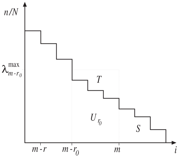
Figure 5: This figure shows a strategy for obtaining the maximum probability of a given $m$-state. The area $T$ is equal to the area $S$. This defines $r_{0}$ and $\lambda_{m-r_{0}}^{\rm max}$

The target area diagram consists of a block of width $m$ with an additional bit on top. This defines $r_{0}$ and $\lambda_{m-r_{0}}^{\rm max}$ (see diagram). The area $S$ has been moved to the area $T$ where these two areas are equal. The height of the main block is $\lambda_{m-r_{0}}^{\rm max}$ which can be calculated since we know that

$$r_{0}\lambda_{m-r_{0}}^{\rm max}=U_{r_{0}}+T=U_{r_{0}}+S=\sum_{i=m-r_{0}+1}^{I}\lambda_{i}$$ (24)

where the last equality follows from the fact that the $i$th column is of area $\lambda_{i}$. The total probability of getting the $m$-state is equal to the area of the main block, i.e. $p_{m}^{\rm max}=m\lambda_{m-r_{0}}^{\rm max}$. We can use this formula if we know what $r_{0}$ is since then $\lambda_{m-r_{0}}^{\rm max}$ can be calculated from (24). This can be established by the following considerations. Define the area $U_{r}$ to consist of all the columns $i=m-r+1$ to $m$ in the start area diagram so that

$$U_{r}=\sum_{i=m-r+1}^{m}\lambda_{i}$$ (25)

where $r=1,2\dots m$. The area $U_{r}+T$ consists of a main block of width $r$ and height $\lambda_{m-r_{0}}^{\rm max}$ plus, for $r\not=r_{0}$, an extra bit lying outside this block (when $r<r_{0}$ a bit of $T$ lies outside this block and when $r>r_{0}$ a bit of $U_{r}$ lies outside the block). Hence,

$$U_{r}+T\geq r\lambda_{m-r_{0}}^{\rm max}$$ (26)

with equality in the case $r=r_{0}$. Therefore,

$$\lambda_{m-r_{0}}^{\rm max}=\min_{r}[{1\over r}(U_{r}+T)]$$ (27)

and we obtain the formula of Lo and Popescu

$$p_{m}^{\rm max}=\min_{r}{m\over r}(\sum_{i=m-r+1}^{I}\lambda_{i})$$ (28)

where $r=1,2,\dots m$. The geometric origin of this formula is now clear.

3 Proof of Nielsen’s Theorem

3.1 Introduction

The set of constraints (9) are exactly Nielsen’s condition [6] for being able to manipulate an entangled state, $|\psi\rangle$, with Schmidt coefficients $\sqrt{\lambda_{i}}$ to another, $|\psi^{\prime}\rangle$, with Schmidt coefficients $\sqrt{\lambda^{\prime}_{i}}$. However, we cannot immediately interpret the new area diagram as being equivalent to a $|\psi^{\prime}\rangle$ state since, unlike in the original area diagram, a given column can be multicoloured. We will see that, nevertheless, we can use the area diagrams to prove Nielsen’s theorem. This proof works along similar lines to the previous proof. First, we put the target state into step form. Alice introduces an ancilla $S$ of dimension $M$ with basis states $|l\rangle_{S}$. If the problem can be solved then, for similar reasons to before, she must be able to manipulate the total state into the form

$$|\Psi_{\rm target}\rangle=\sum_{l}{\sqrt{\mu_{l}}}|l\rangle_{S}|\psi^{\prime}\rangle^{l}$$ (29)

where

$$|\psi^{\prime}\rangle^{l}=\sum_{i=1}^{I}\sqrt{\lambda^{\prime}_{i}}|i\rangle_{A}|i\rangle_{B}^{l}$$ (30)

Substituting (29) into (30) we obtain

$$|\Psi_{\rm target}\rangle=\sum_{l}\sum_{i}\sqrt{\mu_{l}\lambda_{i}}|l\rangle_{S}|i\rangle_{A}|i\rangle_{B}^{l}$$ (31)

Define $M_{li}=\mu_{l}\lambda_{i}M$. We apply the transformation

$$|l\rangle_{S}|i\rangle_{i}\rightarrow{1\over\sqrt{M_{li}}}\sum_{n\in W_{li}}|n\rangle_{S}|i\rangle_{A}$$ (32)

where $W_{li}$ is the set of integers from $(\sum_{k=0}^{l-1}M_{ki})+1$ to $\sum_{k=0}^{l}M_{ki}$ (we set $M_{0i}=0$). Under this transformation (31) becomes

$$|\Psi^{\prime}_{\rm target}\rangle={1\over\sqrt{M}}\sum_{l}\sum_{i}\sum_{n\in W_{li}}|n\rangle_{S}|i\rangle_{A}|i\rangle_{B}^{l}$$ (33)

Each term has equal amplitude in this state. If we project it onto $|n\rangle_{S}$ then we will get a state with, say, $m_{n}$ terms (where $m_{n}$ can be read off from (33)) not all of which are bi-orthogonal. We can relabel the $n$’s so that $m_{n}\geq m_{n+1}$ and hence we can draw an area diagram with a step structure. The terms corresponding to a given $n$ are not necessarily bi-orthogonal and hence we cannot impose on the target area diagram the constraint that elements in a row must all be coloured different colours. Rather we will have a different colouring problem. As before, we will identify the systems $S$ and $R$ so that $M=N$.

3.2 Obtaining Nielsen’s bound

The start state is $|\Psi_{\rm start}\rangle$ in (6) and is represented by an area diagram with step structure in which each column is coloured with only one colour, this being different to the colour of the other columns. The target area diagram is shown in Fig. 6. Since this has been recoloured the columns in this diagram will not necessarily be of one colour. The height of the $i$th column is $\lambda^{\prime}_{i}=N^{\prime}_{i}/N$. We chose a number $Q$ which we will let tend to infinity, though in the Fig. 6 we have set $Q=5$. We divide each column up equally into $Q$ pieces which are numbered $q=1,2,\dots Q$ starting at the bottom.

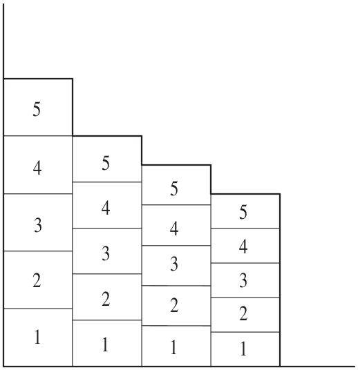
Figure 6: The columns of the target diagram are divided up into $Q$ equal parts. In this figure we have $Q=5$ but we will let $Q\rightarrow\infty$

The $q$th piece in the $i$th column is labelled $[q,i]$ If the target area diagram has been obtained from the start area diagram by moving finite sized bits of area around (as will be the case in our recolouring strategy) then there will be a finite number of horizontal boundaries between different colours. Some of the pieces $[q,i]$ are likely to have these boundaries on them. However, as $Q\rightarrow\infty$ the total area of such pieces will tend to zero and we can assume that each piece has a unique colour. The idea will be to collect all the pieces with a given $q$. Since their areas are proportional to $\lambda^{\prime}_{i}$ they can correspond to the new state $|\psi^{\prime}\rangle^{q}$. However, each of these pieces having the same $q$ must be coloured with a different colour since the terms in $|\psi^{\prime}\rangle^{q}$ are bi-orthogonal. There are $N^{\prime}_{i}$ terms in the state vector corresponding to each column, and since these are divided into $Q$ pieces, there are $N^{\prime}_{i}/Q$ terms corresponding to the $[q,i]$ piece which will be of the form (unnormalised)

$$|[q,i]\rangle={1\over\sqrt{N}}\sum_{n=(q-1)N^{\prime}_{i}/Q+1}^{qN^{\prime}_{i}/Q}|n\rangle_{R}|i\rangle_{A}|j_{qi}\rangle_{B}$$ (34)

The total state is the sum of all such terms. We can transform the total state by applying the transformation

$${\sqrt{Q\over N^{\prime}_{i}}}\sum_{n=(q-1)N^{\prime}_{i}/Q+1}^{qN^{\prime}_{i}/Q}|n\rangle_{R}|i\rangle_{A}\rightarrow|q\rangle_{R}|i\rangle_{A}$$ (35)

for all $q,i$. This sends the term $|[q,i]\rangle$ to the state

$$|[q,i]^{\prime}\rangle=\sqrt{\lambda^{\prime}_{i}\over Q}|q\rangle_{R}|i\rangle_{A}|j_{qi}\rangle_{B}$$ (36)

This transformation has simplified the state of the ancilla $R$ for the terms corresponding to each piece $[q,i]$. In so doing we have recovered the coefficient $\sqrt{\lambda^{\prime}_{i}\over Q}$. The total state is now

$$|\Psi^{\prime}\rangle={1\over\sqrt{Q}}\sum_{q=1}^{I}\sqrt{\lambda^{\prime}_{i}}|q\rangle_{R}|i\rangle_{A}|j_{qi}\rangle_{B}$$ (37)

Now, if we measure onto the $|q\rangle_{R}$ basis we get a state which is a realisation of $|\psi^{\prime}\rangle$ iff the terms are bi-orthogonal. In colouring terms, this means we require that all the pieces labelled with the same $q$ in Fig. 6 should be of different colour. Thus, we have another colouring problem. If we can solve this colouring problem under the assumption that net movement of area is up, then we will have given a constructive proof that Nielsen’s bound can be obtained. To complete the proof of Nielsen’s theorem we need to show that area can only be moved up. This will be done later.

A way to solve this colouring problem was suggested to the author by A. Mahtani. This solution is obtained simply by correcting the solution to the previous colouring problem in Sec. 2.2 [7] Firstly, this colouring procedure, illustrated by example in Fig. 4, is used to go from the start area diagram (representing $|\psi\rangle$) to the target diagram where the heights of the columns are $\lambda^{\prime}_{i}$. Now we note that it is a property of this recolouring procedure that a given colour can end up in two columns at most. There are two ways in which a piece of area can be moved to the left. Either it can be moved directly (as are the pieces $A$ and $D$ in Fig. 4, or it can first be swapped to the right and then be moved back to a further left position than it started in (as are pieces $B$ and $C$ in Fig. 4). We will call the first type directly swapped pieces and the second type of pieces the swapped back pieces. Since these swapped back pieces (for example, piece $B$) must be shorter than the piece that displaced them from their original column (in the case of $B$ this was piece $A$), since they always end up at the top of their destination column, and since the column they end up in is higher than their starting column, they must occupy proportionally less of their final column than the pieces that displaced them (piece $B$ occupies proportionally less of its final column than piece $A$ of its final column). This means that when the columns are divided up into a large number, $Q$, of equal pieces the colours of the swapped back pieces will not appear in two pieces with the same $q$. Hence, we will first correct the other colours. However, the procedure which corrects the colours of the directly swapped pieces disturbs this property of the swapped back pieces. Hence, after correcting for a bunch of directly swapped pieces, we will have to correct for the swapped back pieces as well. First we will consider the colours corresponding to the directly swapped pieces. Before we do that note that some columns will remain unchanged (neither have area moved into them, or out of them) and hence their colour cannot end up in two pieces with the same $q$. These columns can be completely ignored and we can consider only the remaining columns. We start at the rightmost column and go left considering only the columns which have changed. The first changed columns we meet will be shorter than originally, will each be coloured with only one colour, and will have had some area swapped out of them directly. After one or more of these monochromatic columns, we will meet a column into which these directly swapped pieces have been moved. The last directly swapped piece may displace a piece from this column which will be a swapped back piece $S$. This piece, when it is swapped back, will end up at a column, $L$, somewhere to the left. But before we get there, we may meet a few more monochromatic columns, $R_{k}$, from which pieces $X_{k}$ have been directly swapped. We will count $k=K,K-1,\dots 1$ backwards so first we meet $R_{K}$ as we go leftwards. Eventually, on our journey leftwards, we meet column $L$ into which $S$ has been swapped, then pieces $X_{K}$ to $X_{1}$. When the last piece $X_{1}$ is swapped into position it may displace piece $S^{\prime}$ which will be swapped back. Thus, we will repeat the same story as we continue leftwards. Columns will come in bunches of a few monochromatic columns (such as $R_{k}$) followed by a multicoloured column (like $L$). The columns $L$ and $R_{k}$ are shown in Fig. 7(a) for the case $K=3$. Columns not relevant to the present discussion are not shown.

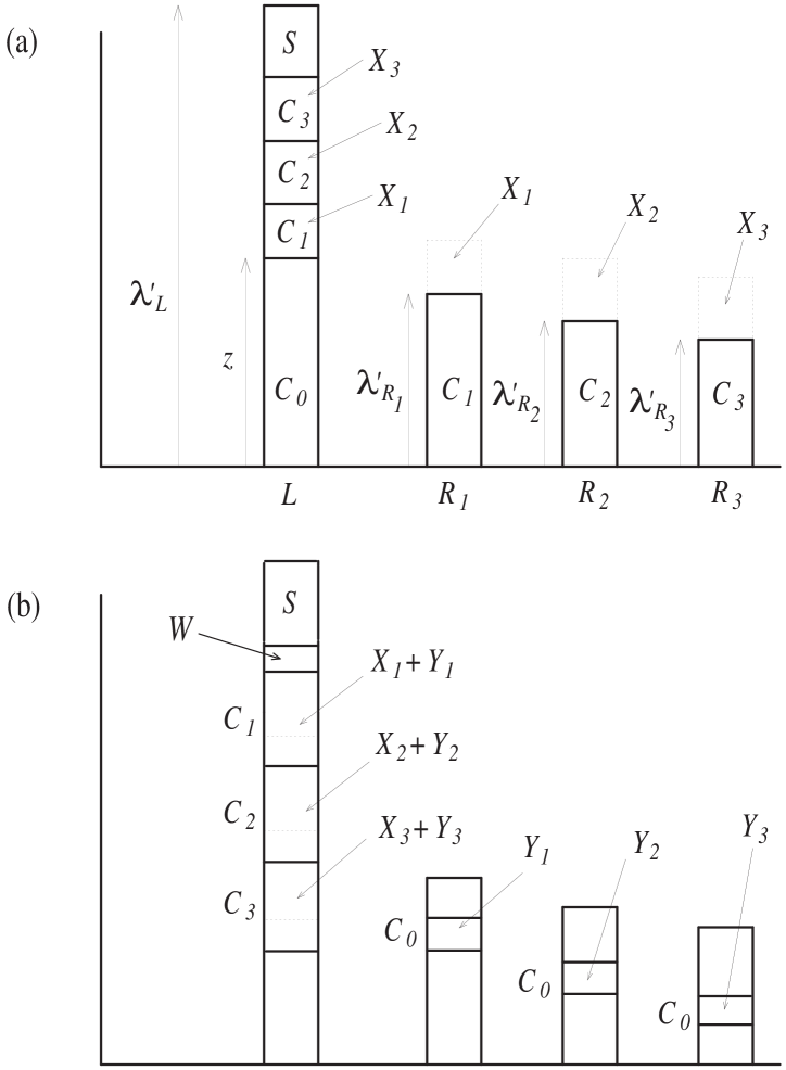
Figure 7: To solve the colouring problem we consider correct bunches of columns such as those shown here. We correct the diagram by moving the areas $Y_{k}$

We label the original colour of $L$ as $C_{0}$ and the colour of $R_{k}$ as $C_{k}$. Various distances (which are numerically equal to areas since the columns are of unit width) are marked on the figure. The strategy we will adopt is the following. We note that, as things stand, the colour $C_{k}$ in all of $R_{k}$ also appears in $L$ and hence, there must be some of the same colour in different columns for the same $q$. To correct this, we can swap an area, $Y_{k}$, of colour $C_{0}$ from $L$ into $R_{k}$ thus swapping the same area, $Y_{k}$, of $C_{k}$ back into $L$. We do this for all $k$. We then re-sort column $L$ so that $Y_{k}$ lies immediately below $X_{k}$, both these areas being of the same colour $C_{k}$ and so that colour $C_{1}$ is above colour $C_{2}$, etc. This is shown in Fig. 7(b) (the role of area $W$ will be explained later). We choose $Y_{K}$ to be such that the proportion of $C_{k}$ in $L$ relative to the height of $L$ is equal to the proportion of $C_{0}$ in $R_{k}$ relative to the height of $R_{k}$. This condition can be expressed as

$${X_{k}+Y_{k}\over\lambda^{\prime}_{L}}={Y_{k}\over\lambda^{\prime}_{R_{k}}}$$ (38)

Furthermore, the area $Y_{k}$ of colour $C_{0}$ is placed in $R_{k}$ at the same relative position of $R_{k}$ as the area $X_{k}+Y_{k}$ of colour $C_{k}$ has been placed in column $L$ (see Fig. 7(b)). This ensures that when the columns are divided up as shown in Fig. 6, but with $Q$ large, the pieces $[q,i_{L}]$ in $L$ of colour $C_{k}$ will have a different colour from the pieces $[q,i_{R_{k}}]$ in $R_{k}$ since the latter pieces will be of colour $C_{0}$.

Having carried out this correcting procedure for these columns we see that there is a problem. Piece $S^{\prime}$ which has been swapped back somewhere to the left of $L$ is of colour $C_{0}$. This piece may overlap (in the sense of occupying some pieces with the same $q$) with the piece $Y_{1}$, also of colour $C_{0}$, which is in column $R_{1}$. We can see $S^{\prime}$ will not also overlap with the pieces $Y_{2},Y_{3},\dots$ (also of colour $C_{0}$) in columns $R_{2},R_{3},\dots$ for the following reasons: (1) It is smaller than $X_{1}$ and hence can only partly overlap with the piece $X_{1}+Y_{1}$ (of colour $C_{1}$) in column $L$ in Fig. 7; (2) This piece of colour $C_{1}$ in column $L$ does not overlap with the colour $C_{0}$ in columns $R_{2},R_{3},\dots$. Hence, this problem only concerns piece $S^{\prime}$ and column $R_{1}$. Let us assume that piece $S^{\prime}$ is in column $L^{\prime}$ and that the original colour of column $L^{\prime}$ is $C^{\prime}_{0}$. We can use colour $C^{\prime}_{0}$ to correct for piece $S^{\prime}$ in $L^{\prime}$ and $Y_{1}$ in $R_{1}$ by essentially the same correcting procedure as before. Thus, we swap a piece of $C^{\prime}_{0}$ and of area $W^{\prime}$ from $L^{\prime}$ to into $Y_{1}$ in $R_{1}$ and at the same time swap a piece of colour $C_{0}$ and of area $W^{\prime}$ from $Y_{1}$ in $R_{1}$ into $L^{\prime}$. The areas $S^{\prime}$ and $W^{\prime}$ are collected together at the top of column $L$. The size of area $W^{\prime}$ is chosen to be just such that $S^{\prime}+W^{\prime}$ (which is of colour $C_{0}$) no longer overlaps with any of the colour $C_{0}$ in $R_{1}$. The maximum size of area $W^{\prime}$ is given by

$${S^{\prime}+W^{\prime}_{\max}\over\lambda^{\prime}_{L^{\prime}}}={W_{\max}\over\lambda^{\prime}_{R_{1}}}$$ (39)

We could have $W^{\prime}$ smaller than the value given by this equation since it is possible that not all of $S^{\prime}$ overlaps with $Y_{1}$ in $R_{1}$. Hence,

$$W^{\prime}\leq{S\lambda^{\prime}_{R_{1}}\over\lambda^{\prime}_{L^{\prime}}-\lambda^{\prime}_{R_{1}}}$$ (40)

This correcting procedure is carried out in the following way. First the rightmost bunch of columns like $R_{k}$ and $L$ are selected. Then the directly swapped pieces are corrected. And then the swapped back pieces are corrected. Then the next bunch of columns are subject to the same correcting protocol until all the bunches have been corrected. If this procedure can be carried out successfully then we will have solved this colouring problem. The only possible problem would be if we had to swap more of the colour $C_{0}$ from $L$ than there is in the column. However, we can show that this will not happen. From the Fig. 7(a) we see that the area, $z$, of the original colour $C_{0}$ in $L$ satisfies

$$\lambda^{\prime}_{L}-\sum_{k=1}^{K}X_{k}-S=z\geq\lambda^{\prime}_{R_{1}}\geq\lambda^{\prime}_{R_{k}}$$ (41)

The inequality must be satisfied since otherwise elements of colour $C_{1}$ in row $L$ will be in the same row as elements of colour $C_{1}$ in row $R_{1}$ but we proved in Sec. II. B. that this could not happen with this colouring of the diagram. From (38,41) we obtain

$$Y_{k}={\lambda^{\prime}_{R_{k}}\over\lambda^{\prime}_{L}-\lambda^{\prime}_{R_{K}}}X_{k}\leq{\lambda^{\prime}_{R_{k}}X_{k}\over\sum_{k^{\prime}}X_{k^{\prime}}+S}\leq{zX_{k}\over\sum_{k^{\prime}}X_{k^{\prime}}+S}$$ (42)

Since $S^{\prime}$ had to be corrected for, $S$ must also be corrected for (if $L$ and $R_{k}$ are taken to represent a general bunch of columns). To correct for $S$ will require an area $W$ of colour $C_{0}$ to be swapped into a column $R^{\prime\prime}_{1}$ somewhere on the right. By analogy with (40) we have

$$W\leq{S\lambda^{\prime}_{R^{\prime\prime}_{1}}\over\lambda^{\prime}_{L}-\lambda^{\prime}_{R^{\prime\prime}_{1}}}\leq{Sz\over\sum_{k^{\prime}}X_{k^{\prime}}+S}$$ (43)

where the second inequality follows since $\lambda^{\prime}_{R^{\prime\prime}_{1}}\leq\lambda_{R_{1}}\leq z$. Hence,

$$\sum_{k}Y_{k}+W\leq z$$ (44)

Which means that there is enough of the colour $C_{0}$ in column $L$ to complete this colouring strategy. Hence, the colouring problem has been solved.

3.3 Proof that Nielsen’s bound cannot be beaten

We need to prove that Nielsen’s bound cannot be beaten. This is equivalent to proving that it is not possible to have net movement of area down the area diagram. The start state corresponds to a step structure. Each column in this can be divided up into $Q$ pieces as shown in Fig. 6. Next we collect together all the pieces corresponding to a given $q$ and place them in order along the $i$ axis as shown in Fig. 8.

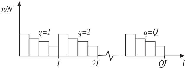
Figure 8: The mini-step form consist of the pieces being arranged along the $i$-axis starting with the $q=1$ pieces.

Thus, going along the $i$ axis we have the $q=1$ pieces, then the $q=2$ pieces and so on. This can be accomplished by Alice performing swap operations. We will call this the mini-step form for the area diagram. (We are, of course, assuming that system $A$ has a large enough Hilbert space to be able to do this. If this is not the case then an additional ancilla could be introduced to effectively increase the size of $A$’s Hilbert space.) Let the state corresponding to this diagram be $|\Psi_{\rm start}^{\rm mini}\rangle$. Now we change from the $(n,i)$ to the $\{n,j\}$ picture where $j$ is the $j$ in $|j\rangle_{B}$. The $\{n,j\}$ element can only be moved up and down the diagram when Alice performs local operations. Hence, in the $\{n,j\}$ picture all the mini-steps will overlay each other so there will be $Q$ elements at each position. The height of the $j$th column will be $N_{j}/Q$. Hence, if we define $A_{nj}=|{}_{B}\langle j|{}_{S}\langle n|\Psi^{\rm mini}\rangle|^{2}$, then for the start state $|\Psi_{\rm start}^{\rm mini}\rangle$ we have

$$\sum_{n=1}^{n^{\prime}}A_{nj}^{\rm start}={n^{\prime}Q\over N}$$ (45)

for all $n^{\prime}\leq N_{j}/Q$. The factor $Q$ comes from the fact that there are $Q$ sets of mini-steps overlaying each other in the $\{n,j\}$ picture.

Now we go back to the $(n,i)$ picture and consider the target state (29). We can apply the transformation

$$|l\rangle_{S}\rightarrow{1\over\sqrt{V_{l}}}\sum_{q\in W_{l}}|q\rangle_{S}$$ (46)

where $V_{l}=\mu_{l}Q$, $W_{l}$ is the set of integers from $(\sum_{r=0}^{l-1}V_{r})+1$ to $\sum_{r=0}^{l}V_{r}$ (we set $V_{0}=0$). We will let $Q\rightarrow\infty$. Under this transformation (29) becomes

$$|\Psi^{\prime\prime}_{\rm target}\rangle={1\over\sqrt{Q}}\sum_{q\in W_{l}}|q\rangle_{S}|\psi^{\prime}\rangle^{q}$$ (47)

where the superscript $q$ is equal to $l$ for $q\in W_{l}$. This state now consists of a number of terms $|q\rangle_{S}|\psi^{\prime}\rangle^{q}$ each having the same amplitude ${1\over\sqrt{Q}}$. Each term, $|q\rangle_{S}|\psi^{\prime}\rangle^{q}$, can individually be put into the step form

$$|q\rangle_{S}|\psi^{\prime}\rangle^{q}\rightarrow|\Psi^{\prime},q\rangle={\sqrt{Q\over N}}\sum_{i}\sum_{n=(q-1)N/Q+1}^{qN/Q}|n\rangle_{S}|i\rangle_{A}|i\rangle_{B}^{q}$$ (48)

by applying transformations similar to (5). If this transformation is applied to all terms then the resulting area diagram will consist of a series of mini-steps lined up vertically as shown in Fig. 9.

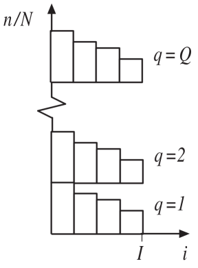
Figure 9: This shows an intermediate state of the area diagram involved in proving that Nielsen’s bound cannot be beaten.

Next, Alice applies swap operations to move these sets of mini-steps so that they are lined up along the $i$ axis starting with the $q=1$ pieces giving an area diagram in mini-step form (like in Fig. 8). The state becomes

$$|\Psi_{\rm target}^{\rm mini}\rangle={\sqrt{1\over N}}\sum_{q}\sum_{j}\sum_{n=1}^{N/Q}|n\rangle_{S}|j+I(q-1)\rangle_{A}|j\rangle_{B}^{q}$$ (49)

For this state we have

$$|{}_{B}\langle\theta|{}_{S}\langle n|\Psi_{\rm target}^{\rm mini}\rangle|^{2}\leq{1\over N}\sum_{q}1={Q\over N}$$ (50)

for any normalised state $|\theta\rangle_{B}$.

The problem is to go from the start diagram in mini-step form to the target diagram which is also in mini-step form. If and only if we can do this can we also go between the corresponding diagrams in standard step form since Alice can transform reversibly between the two types of form of the area diagram. If there is to be net movement of area downwards in the mini-step form then this must happen for at least one value of $j$. Hence, comparing with (45), net downward movement of area implies

$$\sum_{n=1}^{n^{\prime}}A_{nj}^{\rm target}>{n^{\prime}Q\over N}$$ (51)

for at least one value of $j$ and $n^{\prime}<N_{j}/Q$. However, (50) implies

$$\sum_{n=1}^{n^{\prime}}A_{nj}^{\rm target}=\sum_{n=1}^{n^{\prime}}|{}_{B}\langle j|{}_{S}\langle n|\Psi_{\rm target}^{\rm mini}\rangle|^{2}\leq{n^{\prime}Q\over N}$$ (52)

which contradicts (51) and hence there can be no net movement of area downwards in the mini-step form. The standard step form area diagrams are simply elongated versions of one set of mini-steps in the mini-step form, and hence, by the similarity of these shapes, there can be no movement of area downwards in the standard picture. This proves Nielsen’s bound (given algebraically in (9)).

4 Conclusions

In this paper a method of areas has been developed which enables us to understand the manipulation of pure two-particle entanglement. This approach has been used to find the most general way of transforming a general two-particle pure state into maximally entangled states. Certain results of Lo and Popescu were given geometric interpretations. This method has also been used to prove Nielsen’s theorem which pertains to going from one two-particle pure state to another with certainty. There remain a number of open problems relating to manipulation of two-particle pure entanglement which it may be possible to solve using the method of areas. Firstly, we could generalise Nielsen’s theorem to the problem where we go from one state to another but not necessarily with certainty. Secondly, we could consider the problem of going from one state to a distribution of states. The method may also generalise to more than two particles (though it is not presently clear how this generalisation will work).

Acknowledgements

I am grateful to Anna Mahtani for suggesting a way to solve the second colouring problem and to Daniel Jonathan for comments relating to section 2.4 in an earlier version. I would also like to thank the Royal Society for funding.

Note: G. Vidal pointed out to the author that he had already solved [8] the first open problem mentioned in the conclusion. The second open problem has been solved by D. Jonathan and M. Plenio [9] in work done independently of the present work. They also use their result to give a derivation of equation (19).

Appendix

In this appendix we show that there can be no advantage if Alice makes a non-maximal rather than a maximal measurement onto $S$. Assume that the state just before measurement is

$$\sum_{l}c_{l}|l\rangle_{S}|\Phi_{l}\rangle$$ (53)

where $|\Phi_{l}\rangle$ is some state of system $AB$ and not necessarily an $m$-state. Imagine that the projective measurement is non-maximal and one of its projectors is $|1\rangle_{S}\langle 1|+|2\rangle_{S}\langle 2|$. In the case of having the corresponding outcome, the resulting (unnormalised) state will be

$$c_{1}|1\rangle_{S}|\Phi_{1}\rangle+c_{2}|2\rangle_{S}|\Phi_{2}\rangle$$ (54)

This could, for example, be an $m$-state if system $S$ is regarded as being part of system $A$. Rather than performing this non-maximal measurement Alice could instead change her notation for the $|i\rangle_{A}$ states such that, if $|i\rangle_{A}$ appears in the expansions of $|\Phi_{1}\rangle$ and $|\Phi_{2}\rangle$ she writes $|i\rangle_{A}$ as $|1,i\rangle_{A}$. The remaining vectors $|i\rangle_{A}$ are relabelled as $|2,i\rangle_{A}$. We are free to assume that the dimension of $A$ is big enough to do this. Then we write $|k,i\rangle_{A}=|k\rangle_{A^{\prime}}|i\rangle_{A}$. Now Alice performs the transformations

$$|1\rangle_{S}|1\rangle_{A^{\prime}}\rightarrow|2\rangle_{S}|1\rangle_{A^{\prime}}$$ (55)

$$|2\rangle_{S}|1\rangle_{A^{\prime}}\rightarrow|2\rangle_{S}|2\rangle_{A^{\prime}}$$ (56)

Under these transformations the first two terms in (53) become

$$|2\rangle_{S}(c_{1}|1\rangle_{A^{\prime}}|\Phi_{1}\rangle+c_{2}|2\rangle_{A^{\prime}}|\Phi_{2}\rangle)$$ (57)

A maximal measurement will now give rise to a state with the same form as the state as in (54) for the outcome 2. This trick can be repeated everywhere there is a degeneracy in the original non-maximal measurement and a maximal measurement can then be performed instead. This maximal measurement will give rise to the same distribution of the same states as the non-maximal measurement and so there can be no advantage to performing non-maximal measurements.

References

- [1] C. H. Bennett, G. Brassard, C. Crepeau, R. Jozsa, A. Peres, W. K. Wooters, Phys. Rev. Lett. 70, 1895 (1993).
- [2] see C. H. Bennett and P. W. Shor, IEEE Transactions on Information Theory 44, 2724 (1998) and references therein
- [3] R. Cleve and H. Buhrman, Phys. Rev. A 56, 1201 (1997).
- [4] C. H. Bennett, H. J. Bernstein, S. Popescu, and B. Schumacher, Phys. Rev. A. 53, 2046 (1996).
- [5] H-K Lo and S. Popescu, Concentrating entanglement by local actions - beyond mean values, Report No. quant-ph/9707038
- [6] M. A. Nielsen, A partial order on the entangled states, Report No. quant-ph/9811053.
- [7] An alternative solution to this colouring problem can be deduced from the fact, used by Nielsen in [6], that any doubly stochastic matrix may be written as a product of finitely many -transforms. These -transforms correspond to a cut and paste operation on two columns in which the same proportion is cut from each column and added to the other.
- [8] G. Vidal, Entanglement of pure states for a single copy, Report No. quant-ph/9902033. See also G. Vidal, Entanglement monotones, Report No. quant-ph/9807077.
- [9] D. Jonathan and M. Plenio, Minimal conditions for local pure-state entanglement manipulation, Report No. quant-ph/9903054.