Generating entangled superpositions of macroscopically distinguishable states
within a parametric oscillator

Abstract

We suggest a variant of the recently proposed experiment for the generation of a new kind of Schrödinger-cat states, using two coupled parametric down-converter nonlinear crystals $[$F. De Martini, Phys. Rev. Lett. 81, 2842 (1998)$]$. We study the parametric oscillator case and find that an entangled Schrödinger-cat type state of two cavities, whose mirrors are placed along the output beams of the nonlinear crystals, can be realized under suitable conditions.

I Introduction

Schrödinger-cat states [2, 3] are most important in the domain of fundamental quantum mechanics, since the study of their progressive decoherence [4, 5] would provide a better understanding of the transition from the quantum to the classical world [6]. However, due to their extreme sensitivity to the decoherence caused by the interaction with the environment, such linear superpositions of macroscopically distinguishable states are difficult to produce and to observe [4, 5]. In the last few years, a major effort in this field has led to the experimental production and detection of mesoscopic superpositions of distinct states, both in the context of the single-mode microwave cavities [5] and of the dynamics of the center of mass motion of a trapped ion [7]. On the other hand, entanglement has been widely recognized as one of the essential and most puzzling features of quantum mechanics [8], in that it allows the existence of quantum correlated states of two noninteracting subsystems: Entangled states play a crucial role in the so called Einstein, Podolsky and Rosen (EPR) paradox [9], and are essential in the rapidly growing field of quantum information, as they allow the feasibility of quantum state teleportation [10], quantum cryptography [11], and quantum computation [12].

In two recent papers [13], one of us has proposed an original scheme for the generation of a new kind of amplified Schrödinger-cat type states. It is based on the new concept of quantum injection into an optical parametric amplifier (OPA) operating in entangled configuration.

As a relevant variant and a natural extension of the above scheme, in the present work we analyze the case of the quantum injection in an optical parametric oscillator (OPO) in which two optical cavities are added to the OPA scheme considered in Ref. [13]: refer to Fig. 1. Since the presence of the cavities leads to a large enhancement of the nonlinear (NL) parametric interaction, the number of the photon couples which are expected to be generated, in practical conditions, by the OPO scheme is far larger than in the amplifier condition: In addition, the generation of parametrically coupled quasi-coherent fields represents in this context an appealing perspective.

The Schrödinger-cat state that has been put forward in Ref. [13] and is being analyzed, in a more detailed fashion, in the present paper, is a superposition of two macroscopic states which are distinguished by their polarization. It can be considered as a sort of amplified version of the polarization-entangled states which have been widely used in the last few years for the demonstration of the violation of Bell’s inequality [14, 15], of teleportation [10], and for the generation of Greenberger-Horne-Zeilinger (GHZ) states [16].

The present paper is organized as follows: In Sec. II we briefly describe the process of type-II parametric down conversion, with an emphasis on the kind of entangled states usually produced in these experiments, and on the state we want to generate. In Sec. III we outline the experimental apparatus needed for the realization of our scheme. We devote Sec. IV to the presentation of the dynamical time evolution of the density matrix and of the Wigner function in our system, and Sec. V to the discussion of the stability conditions for our parametric oscillator. In Sec. VI we set the initial conditions for the two coupled nonlinear crystals and the two cavities, whereas the way in which the cat state is produced is discussed in detail in Sec. VII. Sec. VIII is devoted to the presentation of the three methods we propose for detecting the Schrödinger-cat state: photodetection (Sec. VIII A), measurement of the second-order quantum coherence (Sec. VIII B), and Wigner function reconstruction (Sec. VIII C). We finally summarize and discuss our results in Sec. IX. The appendix is devoted to the development of the small interaction time approximation.

II Entanglement generating Parametric Down Conversion

Let us first describe the kind of states commonly generated in the experiments aimed at the violation of the Bell’s inequalities. In these experiments the NL crystal (typically beta-barium-borate: BBO) is cut for Type II phase matching where the two down-converted photons are emitted into two cones, one “ordinary” polarized ($o$), the other “extraordinary” polarized ($e$). When the angle between the pump direction and the nonlinear crystal optical axis is sufficiently large [14], the two cones mutually intersect along two lines, lying on opposite sides of the pump beam direction. These ones identify the output modes of the parametric down conversion: $\vec{k}_{j}$ ($j=1$, $2$). Therefore the field belonging to the modes $\vec{k}_{j}$ can be simultaneously $e$- and $o$-polarized. In typical conditions, the output state of the emitted photon couple may be expressed by [10, 13, 17]

$$|\psi\rangle=\frac{1}{\sqrt{2}}\left(|e_{1},o_{2}\rangle+e^{i\phi}|o_{1},e_{2}\rangle\right)\;.$$ (1)

Since we have, for each couple, four degrees of freedom involved, i.e. 2 states of orthogonal linear polarization $e$, $o$ for each mode $\vec{k}_{j}$, we can rewrite state (1) in the more precise form

$$|\psi\rangle=\frac{1}{\sqrt{2}}\left(|1\rangle_{1e}|1\rangle_{2o}|0\rangle_{2e}|0\rangle_{1o}+e^{i\phi}|1\rangle_{1o}|1\rangle_{2e}|0\rangle_{1e}|0\rangle_{2o}\right)\;,$$ (2)

which will be used in the following.

The “Schrödinger-cat state” we want to generate is a sort of amplification of this state, that is, it may be expressed in the form

$$|\psi\rangle = \frac{1}{\sqrt{2}}\left(|\psi^{N}\rangle_{1e}|\psi^{N}\rangle_{2o}|0\rangle_{2e}|0\rangle_{1o}\right.$$ (4)

$$\left.+e^{i\phi}|\psi^{N}\rangle_{1o}|\psi^{N}\rangle_{2e}|0\rangle_{1e}|0\rangle_{2o}\right)\;,$$

where $|\psi^{N}\rangle$ is a state with a large number of photons in some sense, and the states $|0\rangle$ are to be interpreted here as squeezed vacuum states. This kind of state is different from the traditional Schrödinger cat states discussed in the quantum optics literature [4, 5], where one has a single mode of the electromagnetic field in a superposition of two macroscopic states with different phases of the field. The state (4) is a nonlocal superposition in which a macroscopic optical field is “localized” simultaneously either in the $e$- or in the $o$-polarized mode. In other words it is a state more similar to nonlocal field states such as

$$|\psi\rangle=\frac{1}{\sqrt{2}}\left(|\alpha\rangle_{1}|0\rangle_{2}+|0\rangle_{1}|\alpha\rangle_{2}\right)\;,$$ (5)

where the field can be simultaneously in one cavity or in another cavity and whose generation is discussed in [18].

We shall present here an experimental scheme for the generation of a state which is actually a mixed state, but nonetheless, has the same structure of the state of Eq. (4), that is, can be represented by the density operator

$$\rho = \frac{1}{2}\left(\rho(N)_{1e,2o}\otimes\rho(0)_{1o,2e}+\rho(0)_{1e,2o}\otimes\rho(N)_{1o,2e}\right.$$ (8)

$$\left.+\rho({\rm INT})_{1e,2o}\otimes\rho({\rm INT^{\prime}})_{1o,2e}\right.$$

$$\left.+\rho({\rm INT})_{1e,2o}^{\dagger}\otimes\rho({\rm INT^{\prime}})^{\dagger}_{1o,2e}\right)\;,$$

where $\rho(N)$ is a two-mode mixed state with a large number of photons, $\rho(0)$ is a two-mode mixed state with a small number of photons and $\rho({\rm INT})$ and $\rho({\rm INT^{\prime}})$ are the interference terms.

III The experimental scheme

We shall consider an experimental arrangement, Fig. 1, based on the one proposed in Ref. [13] and similar to that adopted in Refs. [19] to show the realization of inducing coherence, without induced emission. Two down-conversion NL crystals, are arranged in such a way that the two corresponding idlers beams are aligned along a common direction $\vec{k}_{2}$. Moreover, both idler beams and the signal beam of one NL crystal (with wave-vector $\vec{k}_{3}$) are placed within couples of mirrors. This scheme can be thought of to realize the coupling of two nondegenerate OPOs. The signal beam of the other crystal, emitted along the direction $\vec{k}_{1}$ triggers the photodetector ${\rm D_{1}}$.

The directions $\vec{k}_{1}$, $\vec{k}_{2}$ and $\vec{k}_{3}$ are selected to realize for both NL crystals the Type-II phase matching described before. These beams are then associated with six modes, with annihilation operator $a_{1o}$, $a_{1e}$, $a_{2o}$, $a_{2e}$, $a_{3o}$ and $a_{3e}$. Note that the first two annihilation operators refer to traveling-waves, while the last four refer to cavity modes.

The dynamics of the system is determined by the nonlinear parametric interaction at each crystal and by the damping terms associated with losses and dissipation inside the cavities [20], as we shall see in the next section.

IV Time evolution for the density matrix and the Wigner function

The partial Hamiltonian operators describing the unitary dynamics inside the crystals are given by [21]

$$\hat{H}_{\rm NL1} = i\hbar\chi_{1}(\hat{a}_{1e}^{\dagger}\hat{a}_{2o}^{\dagger}-\hat{a}_{1e}\hat{a}_{2o})$$ (11)

$$+i\hbar\chi_{1}(\hat{a}_{1o}^{\dagger}\hat{a}_{2e}^{\dagger}-\hat{a}_{1o}\hat{a}_{2e})\;,$$

$$\hat{H}_{\rm NL2} = i\hbar\chi_{2}(\hat{a}_{2o}^{\dagger}\hat{a}_{3e}^{\dagger}-\hat{a}_{2o}\hat{a}_{3e})$$ (13)

$$+i\hbar\chi_{2}(\hat{a}_{2e}^{\dagger}\hat{a}_{3o}^{\dagger}-\hat{a}_{2e}\hat{a}_{3o})\;,$$

where $\chi_{1}=\epsilon_{1}\chi^{(2)}$, $\chi_{2}=\epsilon_{2}\chi^{(2)}$, $\chi^{(2)}$ is the second-order nonlinear susceptibility of the crystals, and $\epsilon_{i}$ ($i=1,2$) is the pump intensity in crystals 1 and 2, respectively, which is assumed to be “classical”.

Due to the explicit presence of dissipation in this problem, one has to write the master equation for the reduced density matrix of the combined system which arises from the Hamiltonian terms (11) and (13) and from the damping terms

$${\cal L}_{i}\rho=\kappa_{i}(2\hat{a}_{i}\rho\hat{a}_{i}^{\dagger}-\hat{a}_{i}^{\dagger}\hat{a}_{i}\rho-\rho\hat{a}_{i}^{\dagger}\hat{a}_{i})\;,$$ (14)

for $i=2e,2o,3e,3o$. Since the damping constants $\kappa_{i}$ are essentially connected to the transmittivity of the mirrors, it is quite natural to assume $\kappa_{2e}=\kappa_{2o}=\kappa_{2}$ and $\kappa_{3e}=\kappa_{3o}=\kappa_{3}$.

Upon writing the full master equation for the total density matrix $\rho_{\rm T}$ of the (six-mode) system, it appears clear that the dynamics of the six modes actually decouples into two independent dynamics for two groups of three modes. In fact, one has

$$\dot{\rho}_{\rm T}={\cal L}_{1e-2o-3e}\rho_{\rm T}+{\cal L}_{1o-2e-3o}\rho_{\rm T}\;,$$ (15)

where

$${\cal L}_{1e-2o-3e}\rho_{\rm T} = -\frac{i}{\hbar}[\hat{H}_{1e-2o-3e},\rho_{\rm T}]$$ (16)

$$+ \kappa_{2}(2\hat{a}_{2o}\rho_{\rm T}\hat{a}_{2o}^{\dagger}-\hat{a}_{2o}^{\dagger}\hat{a}_{2o}\rho_{\rm T}-\rho_{\rm T}\hat{a}_{2o}^{\dagger}\hat{a}_{2o})$$ (17)

$$+ \kappa_{3}(2\hat{a}_{3e}\rho_{\rm T}\hat{a}_{3e}^{\dagger}-\hat{a}_{3e}^{\dagger}\hat{a}_{3e}\rho_{\rm T}-\rho_{\rm T}\hat{a}_{3e}^{\dagger}\hat{a}_{3e})\;,$$ (18)

and

$$\hat{H}_{1e-2o-3e} = i\hbar\chi_{1}(\hat{a}_{1e}^{\dagger}\hat{a}_{2o}^{\dagger}-\hat{a}_{1e}\hat{a}_{2o})$$ (20)

$$+i\hbar\chi_{2}(\hat{a}_{2o}^{\dagger}\hat{a}_{3e}^{\dagger}-\hat{a}_{2o}\hat{a}_{3e})\;.$$

${\cal L}_{1o-2e-3o}$ is identical to ${\cal L}_{1e-2o-3e}$ up to the substitution $e\to o$ and $o\to e$. As a consequence, the complete time evolution will be of the form

$$\rho_{\rm T}(t)=e^{{\cal L}_{1e-2o-3e}t}e^{{\cal L}_{1o-2e-3o}t}\rho_{\rm T}(0)\;.$$ (21)

From Eq. (21) it is clear that if the initial condition is factorized, namely, if

$$\rho_{\rm T}(0)=\rho_{1e-2o-3e}(0)\otimes\rho_{1o-2e-3o}(0)\;,$$ (22)

the state will remain factorized at all times, unless specifically designed conditional measurements [22] are performed on the system (for example on the mode $\vec{k}_{1}$).

Due to the decoupling between the $1e-2o-3e$ and the $1o-2e-3o$ modes, we can simply restrict ourselves to the investigation of the three-mode problem described by the master equation (15) with (16), and we shall drop the subscript $e$ and $o$ when not needed.

The Wigner function [23] $W(x_{1},y_{1},x_{2},y_{2},x_{3},y_{3})=W(\alpha_{1},\alpha_{2},\alpha_{3})$, with $\alpha_{i}=x_{i}+iy_{i}$ $(i=1,2,3)$, resulting from this density matrix $\rho$ will then be a function of six real variables (or three complex variables). Its time evolution, upon evaluating the commutator and the damping terms and after some lengthy algebra, is described by the six-dimensional Fokker-Planck equation

$$\frac{\partial}{\partial t}W(\vec{z},t)=\gamma_{ij}\frac{\partial}{\partial z_{i}}\left(z_{j}W(\vec{z},t)\right)+D_{ij}\frac{\partial}{\partial z_{i}\partial z_{j}}W(\vec{z},t)\;,$$ (23)

where the vector $\vec{z}=(x_{1},y_{1},x_{2},y_{2},x_{3},y_{3})$, the matrix $D={\rm diag}(0,0,\kappa_{2}/4,\kappa_{2}/4,\kappa_{3}/4,\kappa_{3}/4)$, and

$$\gamma=\left(\matrix{0&0&-\chi_{1}&0&0&0\cr 0&0&0&\chi_{1}&0&0\cr-\chi_{1}&0&\kappa_{2}&0&-\chi_{2}&0\cr 0&\chi_{1}&0&\kappa_{2}&0&\chi_{2}\cr 0&0&-\chi_{2}&0&\kappa_{3}&0\cr 0&0&0&\chi_{2}&0&\kappa_{3}}\right)\;.$$ (24)

The solution to Eq. (23) can be written [24] as the integral

$$W(\vec{z},t)=\int d^{4}z^{\prime}\,W(\vec{z}\;^{\prime},0)T(\vec{z},\vec{z}\;^{\prime},t)\;,$$ (25)

where

$$T(\vec{z},\vec{z}\;^{\prime},t) = \frac{1}{(2\pi)^{3}}\frac{1}{\sqrt{{\rm Det}\sigma(t)}}$$ (27)

$$\times \exp\left[-\frac{1}{2}\langle\vec{z}-G(t)\vec{z}\;^{\prime}|\sigma^{-1}(t)|\vec{z}-G(t)\vec{z}\;^{\prime}\rangle\right]\;,$$ (28)

$$G(t) = \exp\left(-\gamma t\right)\;,$$ (29)

and

$$\sigma(t)=2\int\limits_{0}^{t}d\tau\,G(\tau)DG^{t}(\tau)\;,$$ (30)

$G^{t}$ being the transposed of the matrix $G$.

V Stability

The stability properties of the system are intimately connected to the threshold of the overall OPO consisting of NL1 and NL2. Below threshold, the system is stable and reaches a stationary state, since all eigenvalues of $\gamma$ have positive real parts. On the other hand, above threshold the system is unstable and its energy exponentially increases, because some eigenvalues of $\gamma$ have negative real part.

This result can be easily checked in the case in which the parametric oscillator associated with NL2 is decoupled from NL1 ($\chi_{1}=0$): in this case modes $\vec{k}_{2}$ and $\vec{k}_{3}$ decouple from mode $\vec{k}_{1}$, and we end up with a four-dimensional problem for the modes $\vec{k}_{2}$ and $\vec{k}_{3}$, described by a Fokker-Planck equation of the same type as Eq. (23), but with

$$\gamma=\left(\matrix{\kappa_{2}&0&-\chi_{2}&0\cr 0&\kappa_{2}&0&\chi_{2}\cr-\chi_{2}&0&\kappa_{3}&0\cr 0&\chi_{2}&0&\kappa_{3}}\right)\;,$$ (31)

and $D={\rm diag}(\kappa_{2}/4,\kappa_{2}/4,\kappa_{3}/4,\kappa_{3}/4)$. In this case the (doubly degenerate) eigenvalues of $\gamma$ are

$$\lambda_{\pm}=\frac{\kappa_{2}+\kappa_{3}}{2}\pm\sqrt{\left(\frac{\kappa_{2}-\kappa_{3}}{2}\right)^{2}+\chi_{2}^{2}}\;,$$ (32)

and the stability condition becomes

$$\chi_{2}^{2}\leq\kappa_{2}\kappa_{3}\;,$$ (33)

which coincides with the customary threshold for the parametric oscillator [21]. However, if we turn on the first parametric amplifier ($\chi_{1}\neq 0$) then the problem turns from 4-dimensional to 6-dimensional, as we have seen: the eigenvalues of $\gamma$ change and it is in principle possible to change the threshold, i.e., the stability condition. As soon as $\chi_{1}\neq 0$, namely the first parametric amplifier is present, the system becomes unstable, independently on the values of $\chi_{2}$, $\kappa_{2}$, and $\kappa_{3}$. In fact, the eigenvalue equation for $\gamma$ is

$$(\lambda^{3}-(\kappa_{2}+\kappa_{3})\lambda^{2}+(\kappa_{2}\kappa_{3}-\chi_{1}^{2}-\chi_{2}^{2})\lambda+\kappa_{3}\chi_{1}^{2})^{2}=0\;.$$ (34)

As a consequence, we have three doubly degenerate eigenvalues ($\lambda_{1}$, $\lambda_{2}$, and $\lambda_{3}$). Since $\lambda_{1}\lambda_{2}\lambda_{3}=-\kappa_{3}\chi_{1}^{2}$, at least one of the $\lambda_{i}$ has a negative real part.

VI Choice of the initial condition

We assume that at the beginning the first crystal is switched off (the pump strength $\epsilon_{1}=0$). On the other hand, the second pump is on ($\epsilon_{2}\neq 0$) and the second parametric oscillator is in its equilibrium state below threshold. We therefore have a factorized initial state

$$\rho_{\rm T}(0)=\rho_{1e-2o-3e}(0)\otimes\rho_{1o-2e-3o}(0)\;,$$ (35)

where

$$\rho_{1e-2o-3e}(0) = \rho_{1o-2e-3o}(0)=\rho_{1-2-3}(0)$$ (36)

$$= |0\rangle_{1}{}_{1}\langle 0|\otimes\rho_{2-3}(0)\;,$$ (37)

and $\rho_{2-3}(0)$ is the equilibrium state of the oscillator below threshold. This can be easily determined upon considering the limits

$$\lim_{t\to\infty}G(t)=0\;,\,\,\,\,\,\,\,\lim_{t\to\infty}\sigma(t)=\sigma(\infty)\;,$$ (38)

and results in the following expression

$$W(\vec{z},t=\infty) = \int d^{4}z^{\prime}W(\vec{z}\;^{\prime},0)T(\vec{z},\vec{z}\;^{\prime},\infty)$$ (39)

$$= \frac{1}{(2\pi)^{2}}\frac{1}{\sqrt{\det\sigma(\infty)}}\exp\left[-\frac{1}{2}\vec{z}\sigma^{-1}(\infty)\vec{z}\right]\;.$$ (40)

The equilibrium state is thus a Gaussian state in which the modes $\vec{k}_{2}$ and $\vec{k}_{3}$ are correlated.

The initial state $\rho_{2-3}(0)$ is then given by the density matrix corresponding to the Wigner function

$$W^{2-3}_{\rm bt}(0) = \left(\frac{2}{\pi}\right)^{2}\left(1-\frac{\chi_{2}^{2}}{k^{2}}\right)$$ (43)

$$\times\exp\left\{-2\left(x_{2}^{2}+y_{2}^{2}+x_{3}^{2}+y_{3}^{2}-2\frac{\chi_{2}}{k}x_{2}x_{3}\right.\right.$$

$$\left.\left.\,\,\,\,\,\,\,\,\,\,\,\,\,\,\,\,\,\,\,+2\frac{\chi_{2}}{k}y_{2}y_{3}\right)\right\}\;,$$

where it is straightforward to realize that the modes 2 and 3 are correlated. Moreover, it is not a pure state, because

$${\rm Tr}(\rho^{2}) = \pi\int dx_{2}dy_{2}dx_{3}dy_{3}\left[W_{\rm bt}^{2-3}(0)\right]^{2}$$ (44)

$$= \left(1-\frac{\chi_{2}^{2}}{k^{2}}\right)<1\;,$$ (45)

as expected.

The reduced density matrices of each mode are identical and coincide with the thermal state

$$W_{\rm bt}^{\rm red}(0)=\frac{2}{\pi}\left(1-\frac{\chi_{2}^{2}}{k^{2}}\right)\exp\left\{-2|\alpha|^{2}\left(1-\frac{\chi_{2}^{2}}{k^{2}}\right)\right\}\;,$$ (46)

with an initial mean number of photons given by

$$\bar{N}=\frac{\chi_{2}^{2}}{2(k^{2}-\chi_{2}^{2})}\;,$$ (47)

which means that when the oscillator is initially sufficiently close to threshold the initial mean number of photons in modes 2 and 3 within the cavities can be large.

VII Generation of the cat state

At time $t=0$ the first pump is turned on ($\epsilon_{1}\neq 0$): Also the first crystal begins to operate and the two groups of three modes start their joint evolution, according to

$$\rho_{\rm T}(t) = e^{{\cal L}_{1e-2o-3e}t}\rho_{1e-2o-3e}(0)$$ (49)

$$\otimes e^{{\cal L}_{1o-2e-3o}t}\rho_{1o-2e-3o}(0)\;,$$

where the two factorized evolutions are identical because both the operator ${\cal L}$ and the initial condition are identical in the two cases. As a consequence, we end up with two identical six-dimensional problems.

The solution of Eq. (49) can be found as in Sec. IV by using the Wigner functions

$$W_{123}(\vec{z},t)=\int d^{6}z^{\prime}W_{123}(\vec{z}\;^{\prime},0)T(\vec{z},\vec{z}\;^{\prime},t)\;,$$ (50)

where the initial Wigner function $W_{123}(\vec{z},0)$ corresponding to the initial density matrix [Eq. (37)] is given by

$$W_{123}(\vec{z},0) = \left(\frac{2}{\pi}\right)^{3}\left(1-\frac{\chi_{2}^{2}}{k^{2}}\right)e^{-2(x_{1}^{2}+y_{1}^{2})}$$ (54)

$$\times\exp\Big{\{}-2\Big{[}x_{2}^{2}+y_{2}^{2}+x_{3}^{2}+y_{3}^{2}$$

$$\,\,\,\,\,\,\,\,\,\,\,\,\,\,\,\,\,\,\,\,\,-2\left.\left.\frac{\chi_{2}}{k}\left(x_{3}x_{2}+y_{3}y_{2}\right)\right]\right\}$$

$$= \left(\frac{2}{\pi}\right)^{3}\sqrt{\det C}\exp\left\{-2\langle\vec{z}|C|\vec{z}\rangle\right\}\;,$$ (55)

with

$$C=\left(\matrix{1&0&0&0&0&0\cr 0&1&0&0&0&0\cr 0&0&1&0&-\frac{\chi_{2}}{k}&0\cr 0&0&0&1&0&\frac{\chi_{2}}{k}\cr 0&0&-\frac{\chi_{2}}{k}&0&1&0\cr 0&0&0&\frac{\chi_{2}}{k}&0&1\cr}\right)\;,$$ (56)

and

$$\det C=\left(1-\frac{\chi_{2}^{2}}{k^{2}}\right)^{2}\;.$$ (57)

From Eq. (50) one can immediately recognize that since the initial state $W_{123}(\vec{z},0)$ is Gaussian and the propagator $T(\vec{z},\vec{z}\;^{\prime},t)$ is also Gaussian, the Wigner function $W_{123}(\vec{z},t)$ of the evolved state must remain Gaussian at all times.

Upon integrating over $d^{4}z^{\prime}$, Eq. (50) can be rewritten as

$$W(\vec{z},t)=\frac{\sqrt{\det B(t)}}{\pi^{3}}\exp\left\{-\langle\vec{z}|B(t)|\vec{z}\rangle\right\}\;,$$ (58)

where

$$B(t)=\left[2\sigma(t)+\frac{G(t)C^{-1}G^{t}(t)}{2}\right]^{-1}\;,$$ (59)

and $G(t)$ and $\sigma(t)$ are the six-dimensional matrices defined in Eqs. (24), (29), and (30).

This Gaussian evolution holds for a short time only. As a matter of fact, one should distinguish between the mode along direction 1 and those along directions 2 and 3: $a_{2}^{\dagger}$ and $a_{3}^{\dagger}$ denote creation of a photon in the stationary-wave modes within the cavities, whereas $a_{1}^{\dagger}$ denotes the creation of a photon in the traveling-wave mode along direction $\vec{k}_{1}$. Therefore the interaction $H_{\rm NL1}=i\hbar\chi_{1}(a_{1}^{\dagger}a_{2}^{\dagger}-a_{1}a_{2})$ exists only for the time period during which this traveling wave mode 1 moves within the nonlinear crystal. In order to prepare the desired state for the modes 2 and 3, simultaneously taking full advantage of the degree of freedom represented by the traveling-wave mode 1, we perform a conditional [22] measurement on direction 1, thereby conditioning the state of the four modes along directions 2 and 3 upon the detection of a photon along direction 1 polarized at $\pi/4$ with respect to the two output polarizations $e$ and $o$, which are orthogonal to each other. In this way we also post-select (along direction 2) the input state of the second crystal. The projection operator associated to such a conditional measurement is therefore given by

$$\hat{P}_{\frac{\pi}{4}} = \frac{1}{2}\left\{|1\rangle_{1o}|0\rangle_{1e}+|0\rangle_{1o}|1\rangle_{1e}\right\}$$ (61)

$$\times\left\{{}_{1o}\langle 1|{}_{1e}\langle 0|+{}_{1o}\langle 0|{}_{1e}\langle 1|\right\}\;.$$

As a consequence of this measurement (whose success probability amounts to 0.5) the state along direction 1 and directions 2 and 3 factorizes: The state along direction 1 is given by

$$|\psi\rangle_{1}=\frac{1}{\sqrt{2}}\left\{|1\rangle_{1o}|0\rangle_{1e}+|0\rangle_{1o}|1\rangle_{1e}\right\}\;,$$ (62)

which represents a photon polarized at $\pi/4$, whilst the conditional state for directions 2 and 3 is represented by the density matrix

$$\rho^{c}_{2o-3e-2e-3o}(t) \propto \left\{{}_{1o}\langle 1|{}_{1e}\langle 0|+{}_{1o}\langle 0|{}_{1e}\langle 1|\right\}\rho_{1o-2e-3o}(t)$$ (65)

$$\otimes\rho_{1e-2o-3e}(t)\left\{|1\rangle_{1o}|0\rangle_{1e}\right.$$

$$\,\,\,\,\,\,\,\,\,\,\,\,\,\,\,\,\,\,\,\,\,\,\,\,\,\,\,\,\,\,\,\,+\left.|0\rangle_{1o}|1\rangle_{1e}\right\}\;,$$

which can be rewritten as

$$\rho^{c}_{2o-3e-2e-3o}(t) \propto \left[\rho^{(1)}_{2e-3o}\rho^{(0)}_{2o-3e}+\rho^{(0)}_{2e-3o}\rho^{(1)}_{2o-3e}\right.$$ (66)

$$+ \left.\rho^{({\rm int})}_{2e-3o}\rho^{({\rm int})\,\dagger}_{2o-3e}+\rho^{({\rm int})\,\dagger}_{2e-3o}\rho^{({\rm int})}_{2o-3e}\right]\;,$$ (67)

where

$$\rho^{(1)}_{2-3} = {}_{1}\langle 1|\rho_{1-2-3}(t)|1\rangle_{1}\;,$$ (69)

$$\rho^{(0)}_{2-3} = {}_{1}\langle 0|\rho_{1-2-3}(t)|0\rangle_{1}\;,$$ (70)

$$\rho^{({\rm int})}_{2-3} = {}_{1}\langle 1|\rho_{1-2-3}(t)|0\rangle_{1}\;.$$ (71)

The state of Eq. (67) is of the same form of the desired state, Eq. (8), and is a linear superposition of distinguishable states, as long as $\rho^{(1)}_{2-3}$ is well distinguishable from $\rho^{(0)}_{2-3}$.

It should also be emphasized at this stage that the density matrix (67) directly corresponds to the Wigner function, Eq. (2) of Ref. [13], obtained in the OPA case. The similarity between the OPO and the OPA configurations is better brought about in the limit of small interaction times (see the appendix, where it is also shown that—in this limit—many of our results are very similar to those obtained in the OPA case [13]). Roughly speaking, one should recover the OPA results from the OPO ones in the limit $\kappa\to\infty$, since this condition means absence of cavity mirrors. However, this correspondence does not hold exactly because the initial state in the OPO case (the state present in the cavity at $t=0$, when the first nonlinear crystal is switched on) is slightly different. This fact explains the differences between the OPA and the OPO, which result in a far larger effective number of photons in the latter case.

VIII Detection of the cat state

How can we probe the quantum state produced in this parametric-oscillator entangled configuration, and prove that it actually represents a Schrödinger-cat state? In order to do this, one has to independently show that i) the state is indeed made out of two macroscopically distinct components, that ii) these two components exhibit quantum interference, so that the state can be considered as a true linear superposition rather than a statistical mixture, and that iii) the “separation” between the two components scales with a macroscopic or mesoscopic parameter, usually the number of photons. To achieve this goal, we propose three different and independent methods—which can be used either alternatively or simultaneously—as we shall explain in detail in the next three subsections.

A Photodetection

Let us employ photon number measurements for the modes along direction 2, thereby collecting the photon-number distributions $P(n_{2o})$ and $P(n_{2e})$. We therefore consider the reduced density matrix obtained by performing the trace on the state of Eq. (67), that is,

$$\rho_{2e} = {\rm Tr}_{2o-3e-3o}\left\{\rho_{2e-3o-2o-3e}(t)\right\}$$ (72)

$$= \frac{1}{2}\left\{{\rm Tr}_{3o}\left[\rho_{2e-3o}^{(1)}\right]{\rm Tr}_{23}\left[\rho_{2-3}^{(0)}\right]\right.$$ (74)

$$+\left.{\rm Tr}_{3o}\left[\rho_{2e-3o}^{(0)}\right]{\rm Tr}_{23}\left[\rho_{2-3}^{(1)}\right]\right\}\left[P\left(\frac{\pi}{4}\right)\right]^{-1}\;,$$

where $P(\pi/4)$ is the probability of finding one photon with polarization at $\pi/4$, that is,

$$P\left(\frac{\pi}{4}\right) = {\rm Tr}_{1o-1e-2e-3o-2o-3e}\left[\hat{P}_{\frac{\pi}{4}}\rho_{1o-2e-3o}(t)\right.$$ (76)

$$\otimes\left.\rho_{1e-2o-3e}(t)\right]$$

$$= {\rm Tr}_{2-3}\left[\rho_{2-3}^{(1)}\right]{\rm Tr}_{2-3}\left[\rho_{2-3}^{(0)}\right]\;,$$ (77)

represents the probability of the conditional measurement generating the desired cat state. The interference terms in Eq. (67) obviously give no contribution to Eq. (74), since

$${\rm Tr}_{2-3}\left[\rho_{2-3}^{({\rm int})}\right]={\rm Tr}_{2-3}\left[{}_{1}\langle 1|\rho_{1-2-3}(t)|0\rangle_{1}\right]=0\;.$$ (78)

Combining Eqs. (74) and (77), one obtains for the reduced state

$$\rho_{2e}=\frac{1}{2}\left[\frac{{\rm Tr}_{3o}\rho_{2e-3o}^{(1)}}{{\rm Tr}_{2-3}\rho_{2-3}^{(1)}}+\frac{{\rm Tr}_{3o}\rho_{2e-3o}^{(0)}}{{\rm Tr}_{2-3}\rho_{2-3}^{(0)}}\right]\;,$$ (79)

with an identical form for the reduced state $\rho_{2o}$. The reduced density matrices $\rho_{3e}$ and $\rho_{3o}$ can be determined in a similar way.

From Eq. (79) it is immediate to recognize that the reduced state of the mode $2e$ is given by the sum of two density matrices, conditioned upon the detection of one photon and of zero photons in the mode $1o$ (or, more precisely, one photon in the mode $1e$), respectively. Therefore the two terms of the reduced density matrix can be experimentally obtained by rotating the polarizer in front of the detector D₁ located along the direction $\vec{k}_{1}$: When the polarizer is vertical (mode $1e$), we have zero photons in the mode $1o$, and only the second term of the sum in the right-hand side (rhs) of Eq. (79) is realized. On the contrary, if the polarizer is set horizontally (mode $1o$), one detects one photon in the mode $1o$, projecting the resulting density matrix for the mode $2e$ onto the second term in the sum (79). However, both terms are present when the polarizer is set at 45^∘. An experimentalist could then take advantage of this property to test the presence of the two component states: the distinction between the two states in the superposition can be made via photon number measurements, yielding the probability distribution $P(n_{2e})$. In fact, one has

$$P(n_{2e})=\frac{1}{2}\left(P_{\rm H}(n_{2e})+P_{\rm V}(n_{2e})\right)\;,$$ (80)

where $P_{\rm H}(n_{2e})$ [$P_{\rm V}(n_{2e})$] is the probability distribution obtained when the polarized is set horizontally (vertically). The results an experimentalist would obtain with a simple photodetection in these two situations are shown in Fig. 2(a) and (b), together with the probability distribution (80) one would obtain when the polarizer is set at $45^{\circ}$ [Fig. 2(c)].

In this way we have verified the existence of two distinct components in the state (79). But how can we be sure that these two components form a quantum superposition and not just a classical mixture? To answer this question, one has to perform a measurement able to distinguish the “cat state”

$$\rho^{\rm cat}_{2o-3e-2e-3o}(t) = \left[2{\rm Tr}_{2-3}\rho_{2-3}^{(1)}{\rm Tr}_{2-3}\rho_{2-3}^{(0)}\right]^{-1}$$ (81)

$$\otimes \left[\rho^{(1)}_{2e-3o}\rho^{(0)}_{2o-3e}+\rho^{(0)}_{2e-3o}\rho^{(1)}_{2o-3e}\right.$$ (82)

$$+ \left.\rho^{({\rm int})}_{2e-3o}\rho^{({\rm int})\,\dagger}_{2o-3e}+\rho^{({\rm int})\,\dagger}_{2e-3o}\rho^{({\rm int})}_{2o-3e}\right]\;,$$ (83)

from the corresponding statistical mixture

$$\rho^{\rm mix}_{2o-3e-2e-3o}(t) = \left[2{\rm Tr}_{2-3}\rho_{2-3}^{(1)}{\rm Tr}_{2-3}\rho_{2-3}^{(0)}\right]^{-1}$$ (84)

$$\times \left[\rho^{(1)}_{2e-3o}\rho^{(0)}_{2o-3e}+\rho^{(0)}_{2e-3o}\rho^{(1)}_{2o-3e}\right]\;,$$ (85)

which does not exhibit any interference.

In order to reach this goal, we perform an interference experiment, involving the modes along direction $\vec{k}_{2}$ only, using a detection system similar to the one proposed in Ref. [13], as schematically described in Fig. 1. The measured quantity is given by the photocounts at the detector D_c, as a function of the variable phase $\phi$. The annihilation operator $c$ corresponding to the mode traveling to the detector D_c can be written in terms of the annihilation operators of the modes $2e$ and $2o$ as

$$c=\frac{1}{\sqrt{2}}\left(a_{2o}+e^{i\phi}a_{2e}\right)\;,$$ (86)

so that the operator number of photons for the mode $c$ will be given by

$$c^{\dagger}c=\frac{1}{2}\left(a_{2o}^{\dagger}a_{2o}+a_{2e}^{\dagger}a_{2e}+e^{i\phi}a_{2o}^{\dagger}a_{2e}+e^{-i\phi}a_{2e}^{\dagger}a_{2o}\right)\;.$$ (87)

In order to be able to distinguish between the superposition state and the mixture, the expectation value

$$\langle c^{\dagger}c\rangle_{\rm cat}={\rm Tr}\left[c^{\dagger}c\rho_{2o-3e-2e-3o}^{\rm cat}(t)\right]$$ (88)

has to be different from

$$\langle c^{\dagger}c\rangle_{\rm mix}={\rm Tr}\left[c^{\dagger}c\rho_{2o-3e-2e-3o}^{\rm mix}(t)\right]\;.$$ (89)

It is then clear that this interference experiment can answer our question whenever the contributions of the off-diagonal terms ${\rm Tr}[c^{\dagger}c\rho_{2e-3o}^{\rm(int)}\rho_{2o-3e}^{\rm(int)\,\dagger}]$ and its complex conjugate ${\rm Tr}[c^{\dagger}c\rho_{2e-3o}^{\rm(int)\,\dagger}\rho_{2o-3e}^{\rm(int)}]$ are nonzero.

Let us start by evaluating the contribution of the diagonal terms, namely, Eq. (89). After explicit integration of the corresponding Wigner function, it is easy to prove that the phase-dependent terms [the third and the fourth term in Eq. (87)] vanish when one computes the expectation value, Eq. (89). Therefore the diagonal terms yield a phase ($\phi$)-independent contribution given by

$$\langle c^{\dagger}c\rangle_{\rm mix} = \frac{1}{2}\left(\langle a_{2o}^{\dagger}a_{2o}\rangle_{\rm mix}+\langle a_{2e}^{\dagger}a_{2e}\rangle_{\rm mix}\right)$$ (91)

$$= \frac{1}{4}\left[\langle n_{2o}\rangle^{(1)}+\langle n_{2o}\rangle^{(0)}\right]$$ (93)

$$+\frac{1}{4}\left[\langle n_{2e}\rangle^{(1)}+\langle n_{2e}\rangle^{(0)}\right]$$

$$= \frac{1}{2}\left[\langle n_{2}\rangle^{(1)}+\langle n_{2}\rangle^{(0)}\right]\;,$$ (94)

where

$$\langle n_{2}\rangle^{(i)}=\frac{{\rm Tr}_{2-3}\left[\rho_{2-3}^{(i)}a_{2}^{\dagger}a_{2}\right]}{{\rm Tr}_{2-3}\left[\rho_{2-3}^{(i)}\right]}\;,$$ (95)

($i=0$, 1) is the mean photon number in one of the two diagonal states in Eqs. (83) and (85). In the small interaction-time limit, which is very well justified in the present case (see appendix), $1\gg kt$, $\chi_{1}t$, $\chi_{2}t$, we have

$$\rho_{2-3}^{(0)} \simeq \rho_{2-3}(0)\;,$$ (97)

$$\rho_{2-3}^{(1)} \propto a_{2}^{\dagger}\rho_{2-3}(0)a_{2}\;.$$ (98)

As a consequence, the two expectation values in the rhs of Eq. (94) can be explicitly evaluated and are given by

$$\langle n_{2}\rangle^{(0)} = \bar{N}=\left[2\left(\frac{k^{2}}{\chi_{2}^{2}}-1\right)\right]^{-1}\;,$$ (100)

$$\langle n_{2}\rangle^{(1)} = 2\bar{N}+1\;,$$ (101)

where $\bar{N}$ is the initial mean photon number in the cavity. In conclusion, the diagonal contribution to the expectation value in Eq. (88) amounts to

$$\langle c^{\dagger}c\rangle_{\rm mix}\simeq\frac{1+3\bar{N}}{2}\;,$$ (102)

which is indeed $\phi$-independent as expected.

We turn now our attention to the off-diagonal terms in Eq. (83), which are absent in Eq. (85). First we note that the expectation values of the number operators relative to the two polarizations in mode 2 computed on the off-diagonal terms vanish, i.e.,

$$\langle a_{2o}^{\dagger}a_{2o}\rangle_{\rm o-d}=\langle a_{2e}^{\dagger}a_{2o}\rangle_{\rm o-d}=0\;.$$ (103)

On the other hand, the third and the fourth term in the rhs of Eq. (87) give to the expectation value on the off-diagonal terms the contributions

$$e^{i\phi}\langle a_{2o}^{\dagger}a_{2e}\rangle_{\rm o-d} = \left\{2{\rm Tr}_{2-3}\left[\rho_{2-3}^{(1)}\right]{\rm Tr}_{2-3}\left[\rho_{2-3}^{(0)}\right]\right\}^{-1}$$ (107)

$$\times\left(\langle a_{2e}\rangle^{\rm(int)}\langle a_{2o}^{\dagger}\rangle^{{\rm(int)}\,\dagger}\right.$$

$$\,\,\,\,\,\,\,\,\,+\left.\langle a_{2e}\rangle^{{\rm(int)}\,\dagger}\langle a_{2o}^{\dagger}\rangle^{\rm(int)}\right)\;,$$

$$e^{-i\phi}\langle a_{2e}^{\dagger}a_{2o}\rangle_{\rm o-d} = \left(e^{i\phi}\langle a_{2o}^{\dagger}a_{2e}\rangle_{\rm o-d}\right)^{*}\;,$$ (108)

where

$$\langle a_{2}\rangle^{\rm(int)}={\rm Tr}_{2-3}\left[\rho_{2-3}^{\rm(int)}a_{2}\right]\;.$$ (109)

These contributions are generally different from zero, and this observation is sufficient to reach the conclusion that the proposed interference experiment is able to distinguish the cat state from the corresponding mixture.

We are able to evaluate these off-diagonal terms in the small interaction-time limit developed in the appendix: At the lowest order in $\chi_{1}t$, $\chi_{2}t$, and $kt$, we have

$$\rho_{2-3}^{\rm(int)}\simeq a_{2}^{\dagger}\rho_{2-3}(0)\;,$$ (110)

and therefore, using Eq. (109),

$$\langle a_{2e}\rangle^{\rm(int)} = \chi_{1}t\left(\bar{N}+1\right)\;,$$ (112)

$$\langle a_{2e}\rangle^{{\rm(int)}\,\dagger} = \chi_{1}t\langle a_{2e}^{2}\rangle=0\;,$$ (113)

$$\langle a_{2o}^{\dagger}\rangle^{\rm(int)} = \chi_{1}t\langle a_{2o}^{\dagger\,2}\rangle=0\;,$$ (114)

$$\langle a_{2o}^{\dagger}\rangle^{{\rm(int)}\,\dagger} = \chi_{1}t\left(\bar{N}+1\right)\;.$$ (115)

On the other hand,

$$\rho_{2-3}^{(1)} \simeq \chi_{1}^{2}t^{2}a_{2}^{\dagger}\rho_{2-3}(0)a_{2}\;,$$ (117)

$$\rho_{2-3}^{(0)} \simeq \rho_{2-3}(0)\;,$$ (118)

which yield, respectively,

$${\rm Tr}_{2-3}\rho_{2-3}^{(1)} = \chi_{1}^{2}t^{2}\left(\bar{N}+1\right)\;,$$ (120)

$${\rm Tr}_{2-3}\rho_{2-3}^{(0)} \simeq 1\;,$$ (121)

and, finally,

$$e^{i\phi}\langle a_{2o}^{\dagger}a_{2e}\rangle_{\rm o-d}=\frac{\bar{N}+1}{2}e^{i\phi}\;.$$ (122)

In conclusion, considering the off-diagonal contribution, Eq. (88) can be rewritten as

$$\langle c^{\dagger}c\rangle_{\rm cat}=\langle c^{\dagger}c\rangle_{\rm mix}+\frac{\bar{N}+1}{2}\cos\phi\;.$$ (123)

It is then clear that the photocounts at the detector D_c exhibit interference fringes as a function of the variable phase $\phi$, if and only if the state (79) is a true linear superposition and not just a statistical mixture of the two macroscopic components. The visibility of such interference fringes is given by

$$V=\frac{1+\bar{N}}{1+3\bar{N}}$$ (124)

and has therefore the lower bound $1/3$ for $\bar{N}\to\infty$.

B Correlation functions

Our aim in this subsection is to compute the first- and second-order correlation functions relative to our output modes, in order to make an independent test of the presence of quantum coherence in our system. We keep in mind [26] that a manifestation of quantum coherence at second order is subpoissonian statistics, i.e.,

$$G^{(2)}(0)<\left[G^{(1)}(0)\right]^{2}\;,$$ (125)

where $G^{(1)}(0)$ and $G^{(2)}(0)$ are, respectively, the first- and second-order correlation functions.

Let us consider the same experimental apparatus we have proposed for the detection of interference (see Fig. 1). We take now into account both output ports $c$ and $d$ of the polarizing beam splitter, with annihilation operators

$$c=\frac{1}{\sqrt{2}}\left(a_{2o}+e^{i\phi}a_{2e}\right)\;,$$ (127)

$$d=\frac{1}{\sqrt{2}}\left(a_{2o}-e^{i\phi}a_{2e}\right)\;,$$ (128)

and evaluate the correlation functions $\langle c^{\dagger}cc^{\dagger}c\rangle$, $\langle d^{\dagger}dd^{\dagger}d\rangle$, and $\langle c^{\dagger}cd^{\dagger}d\rangle$, where $c^{\dagger}c$ is given by Eq. (87), and

$$d^{\dagger}d=\frac{1}{2}\left(a_{2o}^{\dagger}a_{2o}+a_{2e}^{\dagger}a_{2e}-e^{i\phi}a_{2o}^{\dagger}a_{2e}-e^{-i\phi}a_{2e}^{\dagger}a_{2o}\right)\;.$$ (129)

We shall evaluate the functions $(c^{\dagger}c)^{2}$, $(d^{\dagger}d)^{2}$, and $c^{\dagger}cd^{\dagger}d$ in the small-time approximation limit (see appendix), in which

$$\rho_{2e-3o-2o-3e}(t) \propto \left(a_{2e}^{\dagger}+a_{2o}\dagger\right)\rho_{2e-3o}(0)\rho_{2o-3e}(0)$$ (131)

$$\times\Big{(}a_{2e}+a_{2o}\Big{)}\;,$$

where $\rho_{2o-3e}(0)$ is the Gaussian state described by the Wigner function $W_{\rm bt}^{2-3}(0)$ of Eq. (43), for which the Wigner function corresponding to the reduced density matrix of mode $2$ alone is given by Eq. (46), that represents a thermal state with a mean number of photons given by $\bar{N}$ of Eq. (100).

Upon evaluating all the required expectation values, we obtain

$$\langle\left(c^{\dagger}c\right)^{2}\rangle = \frac{16\bar{N}^{2}+14\bar{N}+2+2\cos\phi\left(4\bar{N}^{2}+5\bar{N}+1\right)}{4}$$ (133)

$$\langle\left(d^{\dagger}d\right)^{2}\rangle = \frac{16\bar{N}^{2}+14\bar{N}+2-2\cos\phi\left(4\bar{N}^{2}+5\bar{N}+1\right)}{4}$$ (135)

$$\langle c^{\dagger}cd^{\dagger}d\rangle = \bar{N}\left(2\bar{N}+1\right)\;.$$ (137)

From Eqs. (VIII B) it is clear that the visibility of the fringes in $\langle(c^{\dagger}c)^{2}\rangle$ and $\langle(d^{\dagger}d)^{2}\rangle$ is given by

$$V=\frac{4\bar{N}^{2}+5\bar{N}+1}{8\bar{N}^{2}+7\bar{N}+1}\;,$$ (138)

and monotonically decreases from $V=1$ (for $\bar{N}=0$) to $V=1/2$ (for $\bar{N}\to\infty$).

Finally, considering the field at the output port $c$, the first- and second-order correlation functions for mode $2$ can be written as

$$G^{(1)}_{2}(0) = \langle c^{\dagger}c\rangle=\frac{1+3\bar{N}+(1+\bar{N})\cos\phi}{2}\;,$$ (140)

$$G^{(2)}_{2}(0) = \langle c^{\dagger}c^{\dagger}cc\rangle=\langle\left(c^{\dagger}c\right)^{2}\rangle-\langle c^{\dagger}c\rangle$$ (141)

$$= 2\bar{N}\left[1+2\bar{N}+\left(\bar{N}+1\right)\cos\phi\right]\;,$$ (142)

respectively. It should be noted that these results map into the corresponding ones obtained in Ref. [13] for the OPA case upon a redefinition of the phase angles. By comparing $[G^{(1)}(0)]^{2}$ and $G^{(2)}(0)$ it is possible to see that $G^{(2)}(0)<[G^{(1)}(0)]^{2}$ only at low mean photon number, as it could have been easily expected. The best situation is obtained when $\phi=0$, in which case

$$[G^{(1)}(0)]^{2} = \left(1+2\bar{N}\right)^{2}\;,$$ (144)

$$G^{(2)}(0) = 2\bar{N}\left(3\bar{N}+2\right)\;,$$ (145)

and the condition for quantum coherence at second order is reached when $\bar{N}<1/\sqrt{2}$. On the other hand, when $\phi=\pi$, $[G^{(1)}(0)]^{2}=\bar{N}^{2}$, $G^{(2)}(0)=2\bar{N}^{2}$, and therefore $G^{(2)}(0)$ is always larger than $[G^{(1)}(0)]^{2}$.

C Wigner function

The aim of the present section is to provide a means to represent the essential features of the Schrödinger-cat state, Eq. (67), which “lives” in a 8-dimensional phase space, in the more customary 2-dimensional phase space, in order to make a comparison with the more conventional cat states [3, 5]. Let us start from Eq. (67) which we rewrite here for convenience

$$\rho^{c}_{2o-3e-2e-3o}(t) \propto \left[\rho^{(1)}_{2e-3o}\rho^{(0)}_{2o-3e}+\rho^{(0)}_{2e-3o}\rho^{(1)}_{2o-3e}\right.$$ (146)

$$+ \left.\rho^{({\rm int})}_{2e-3o}\rho^{({\rm int})\,\dagger}_{2o-3e}+\rho^{({\rm int})\,\dagger}_{2e-3o}\rho^{({\rm int})}_{2o-3e}\right]\;.$$ (147)

The Wigner function representation of the density matrix (147) would of course reflect its characteristic Schrödinger-cat properties. However, in order to better understand the nature of this state, it would be interesting and desirable to see whether it is possible to find different optical modes in whose terms the state (and therefore the Wigner function) may be rewritten in a simpler form. Our key idea is then to look for linear combinations of mode operators (which can easily be realized with linear elements: polarizers and beam-splitters) such as to factorize the state (147) in smaller subspaces.

We first perform a transformation which changes the horizontally and vertically polarized modes into the 45^∘-polarized ones, namely,

$$a_{+45,2} = \frac{a_{2e}+a_{2o}}{\sqrt{2}}\;,\;\;\;a_{-45,2}=\frac{a_{2e}-a_{2o}}{\sqrt{2}}\;,$$ (149)

$$a_{+45,3} = \frac{a_{3e}+a_{3o}}{\sqrt{2}}\;,\;\;\;a_{-45,3}=\frac{a_{3e}-a_{3o}}{\sqrt{2}}\;,$$ (150)

and the corresponding expressions for mode $\vec{k}_{1}$ and for the creation operators. In terms of these new operators, $H_{\rm NL1}$ and $H_{\rm NL2}$ [Eqs. (11) and (13)] can be rewritten as

$$H_{\rm NL1} = i\hbar\chi_{1}\left({a}_{+45,2}^{\dagger}{a}_{+45,1}^{\dagger}-{a}_{+45,2}{a}_{+45,1}\right)$$ (153)

$$-i\hbar\chi_{1}\left({a}_{-45,2}^{\dagger}{a}_{-45,1}^{\dagger}-{a}_{-45,1}{a}_{-45,2}\right)\;,$$

$${H}_{\rm NL2} = i\hbar\chi_{2}\left({a}_{+45,2}^{\dagger}{a}_{+45,3}^{\dagger}-{a}_{+45,2}{a}_{+45,3}\right)$$ (155)

$$-i\hbar\chi_{2}\left({a}_{-45,2}^{\dagger}{a}_{-45,3}^{\dagger}-{a}_{-45,2}{a}_{-45,3}\right)\;.$$

We have already assumed [Sec. IV] that the cavity decay rates $\kappa_{i}$ do not depend on the polarization. This in turn means that $\kappa_{+45,2}=\kappa_{-45,2}=\kappa_{2}$ and $\kappa_{+45,3}=\kappa_{-45,3}=\kappa_{3}$, and therefore we have that for the $\pm 45^{\circ}$-polarized modes we have the same evolution equation as that for the original modes (except for a minus sign). Consequently, it is possible to repeat all the same arguments as before [Secs. IV and VII]. In particular, the modes $a_{+45,1}$, $a_{+45,2}$, and $a_{+45,3}$ are decoupled from their orthogonal counterparts $a_{-45,1}$, $a_{-45,2}$, and $a_{-45,3}$, and the evolution equation may be rewritten as

$$\rho_{\rm T}(t)=e^{{\cal L}_{+45}t}e^{{\cal L}_{-45}t}\rho_{+45,1;+45,2;+45,3;-45,1;-45,2;-45,3}(0)\;.$$ (156)

In Eq. (156) the initial condition is given in the same way by

$$\rho_{+45,1;+45,2;+45,3}(0)=|0\rangle_{+45,1}\langle 0|\otimes\rho^{\rm bt}_{+45,2;+45,3}(0)\;,$$ (157)

where $\rho^{\rm bt}_{+45,2;+45,3}(0)$ is the equilibrium state below threshold of the parametric oscillator when NL1 is turned off, and the same initial condition holds for the $-45^{\circ}$-polarized modes. As a consequence, the same Gaussian evolution we have found in Sec. IV holds. The only difference is that now the conditional measurement is simply a projection onto the state $|1\rangle_{+45,1}$, i.e., the one-photon state for the $a_{+45,1}$ mode, while the $-45^{\circ}$-polarized modes remain decoupled from the orthogonal ones.

The cat state after the conditional detection of the $n=1$ photon for the $+45,1$ mode is then written in the following way

  

$$\rho^{\rm c} \propto {}_{-45,1}\langle 0|_{+45,1}\langle 1|\rho_{+45,1;+45,2;+45,3}(t)\rho_{-45,1;-45,2;-45,3}|1\rangle_{+45,1}|0\rangle_{-45,1}=\rho_{+45,2;+45,3}^{(1)}\otimes\rho_{-45,2;-45,3}^{(0)}\;,$$ (158)

 

 

where $\rho_{2-3}^{(0)}$ and $\rho_{2-3}^{(1)}$ are again given by the expressions (69) and (70). It should be noted that, using these new $\pm 45^{\circ}$-polarized modes, one gets a complete factorization of the $-45^{\circ}$-polarized modes, which are not affected by the quantum injection process induced by the conditional measurement. The $-45^{\circ}$-polarized modes are not “interesting”, in the sense that all the “cat” properties of the state (158) are contained in $\rho_{+45,2;+45,3}^{(1)}$, and therefore we shall neglect them from now on. We are then left with the state $\rho_{+45,2;+45,3}^{(1)}$, which is an entangled state of the modes $+45,2$ and $+45,3$.

As the second step of our procedure aimed at the further simplification of the original 8-dimensional Wigner function, we consider the transformation

$$d_{+}=\frac{a_{+45,2}+a_{+45,3}}{\sqrt{2}}\;,\;\;\;d_{-}=\frac{a_{+45,2}-a_{+45,3}}{\sqrt{2}}\;,$$ (159)

which is suggested by the interaction term in Eq. (155). In terms of $d_{+}$ and $d_{-}$, Eq. (155) becomes

$$H_{\rm NL2}=i\hbar\frac{\chi_{2}}{2}\left(d_{+}^{\dagger\,2}-d_{+}^{2}\right)-i\hbar\frac{\chi_{2}}{2}\left(d_{-}^{\dagger\,2}-d_{-}^{2}\right)\;,$$ (160)

and the two modes $d_{+}$ and $d_{-}$ are squeezed by the nonlinear crystal. These modes can be experimentally realized outside the cavity for example with two PBS and a 50%–50% BS, as schematically described in Fig. 3. The state of these two modes can be represented by the Wigner function

$$W_{1}\left(\frac{x_{d_{+}}+x_{d_{-}}}{\sqrt{2}},\frac{y_{d_{+}}+y_{d_{-}}}{\sqrt{2}},\frac{x_{d_{+}}-x_{d_{-}}}{\sqrt{2}},\frac{y_{d_{+}}-y_{d_{-}}}{\sqrt{2}}\right)\;,$$ (161)

where [see Eqs. (58) and (59)]

  

$$W_{1}\left(x_{2},y_{2},x_{3},y_{3}\right) \propto \int dx_{1}dy_{1}\,W_{n=1}\left(x_{1},y_{1}\right)\times\frac{\sqrt{\det B}}{\pi^{2}}e^{-\langle\vec{z}|B|\vec{z}\rangle}\;.$$ (162)

What is the nature of this state? In order to answer this question, we are naturally guided by two different approaches: i) the study of the OPA case [13] and ii) the use of the small-time limit $\chi_{1}t,\chi_{2}t,\kappa t\ll 1$ we have already considered in Sec. VIII A and worked out in the appendix. In the OPA case [13] the output state at time $t$ is given by

$$|\psi(t)\rangle = \frac{1}{\sqrt{2}}e^{\chi_{2}t(a_{2e}^{\dagger}a_{3o}^{\dagger}-a_{2e}a_{3o})+\chi_{2}t(a_{2o}^{\dagger}a_{3e}^{\dagger}-a_{2o}a_{3e})}\times\left(a_{2e}^{\dagger}+a_{2o}^{\dagger}\right)|0\rangle\;,$$ (163)

which can be rewritten in terms of the $\pm 45^{\circ}$-polarized modes as

$$|\psi(t)\rangle = e^{-\chi_{2}t(a_{-45,2}^{\dagger}a_{-45,3}^{\dagger}-a_{-45,2}a_{-45,3})}|0\rangle\otimes e^{\chi_{2}t(a_{+45,2}^{\dagger}a_{+45,3}^{\dagger}-a_{+45,2}a_{+45,3})}a_{+45,2}^{\dagger}|0\rangle=\psi_{-45,2;-45,3}^{(0)}\psi_{+45,2;+45,3}^{(1)}\;.$$ (164)

Neglecting the factorized state $\psi_{-45,2;-45,3}^{(0)}$, and using the $d_{\pm}$ modes, we have

$$\psi_{+45,2;+45,3}^{(1)} = e^{\frac{\chi_{2}t}{2}(d_{+}^{\dagger\,2}-d_{+}^{2})}e^{-\frac{\chi_{2}t}{2}(d_{-}^{\dagger\,2}-d_{-}^{2})}\left(\frac{d_{+}^{\dagger}+d_{-}^{\dagger}}{\sqrt{2}}\right)|0\rangle$$ (166)

$$= \frac{1}{\sqrt{2}}\left(\left|\frac{\chi_{2}t}{2},1\right\rangle_{d_{+}}\left|-\frac{\chi_{2}t}{2},0\right\rangle_{d_{-}}\right.+\left.\left|\frac{\chi_{2}t}{2},0\right\rangle_{d_{+}}\left|-\frac{\chi_{2}t}{2},1\right\rangle_{d_{-}}\right)\;,$$ (167)

 

 

which is an entangled superposition of the squeezed one-photon and vacuum states of the modes $d_{+}$ and $d_{-}$. It is quite clear now that if we want to “isolate” one mode, say, the $d_{+}$ mode, we need a second conditional measurement on the mode $d_{-}$, e.g., a projection onto the state

$$|\varphi\rangle_{d_{-}}=\alpha|0\rangle_{d_{-}}+\beta|1\rangle_{d_{-}}\;.$$ (168)

Such a conditional measurement could be performed, for example, by sending a two-level atom—resonant with the atomic transition—through the cavity, and eventually post-selecting its internal state in a corresponding superposition of its ground and excited states. The conditional state, provided the measurement has given a successful result, would then read as

$$|\psi^{\rm c}\rangle_{d_{+}}\propto\alpha^{\star}|\frac{\chi_{2}t}{2},1\rangle_{d_{+}}+\frac{\beta^{\star}}{\cosh\chi_{2}t}|\frac{\chi_{2}t}{2},0\rangle_{d_{+}}\;.$$ (169)

We can reach a similar conclusion also by analyzing the OPO case using the very well justified small-time approximation (see appendix) in the limit $\chi_{1}t,\chi_{2}t,\kappa t\ll 1$, applied to the modes $+45,1$, $+45,2$, and $+45,3$. We have, at the lowest order in $\chi_{1}t$,

$$\rho_{+45,2;+45,3}^{(1)} = {}_{+45,1}\langle 1|\rho_{1-2-3}|1\rangle_{+45,1}$$ (171)

$$\propto a_{+45,2}^{\dagger}\rho_{2-3}(0)a_{+45,2}\;,$$ (172)

where the initial density matrix $\rho_{2-3}(0)$ is the state described by the Wigner function (43). If we now write Eq. (43) in terms of the new variables corresponding to the modes $d_{+}$ and $d_{-}$, namely,

$$x_{d_{+}} = \frac{x_{2}+x_{3}}{\sqrt{2}}\;,\;\;\;\;\;\;x_{d_{-}}=\frac{x_{2}-x_{3}}{\sqrt{2}}\;,$$ (174)

$$y_{d_{+}} = \frac{y_{2}+y_{3}}{\sqrt{2}}\;,\;\;\;\;\;\;x_{d_{-}}=\frac{y_{2}-y_{3}}{\sqrt{2}}\;,$$ (175)

we obtain

  

$$W_{\rm bt}^{d_{+}d_{-}} = W_{\rm bt}^{d_{+}}W_{\rm bt}^{d_{-}}=\frac{2}{\pi}\sqrt{1-\frac{\chi_{2}^{2}}{\kappa^{2}}}\exp\left[-2\left(1-\frac{\chi_{2}}{\kappa}\right)x_{d_{+}}^{2}\right.\left.-2\left(1+\frac{\chi_{2}}{\kappa}\right)y_{d_{+}}^{2}\right]$$ (177)

$$\times\frac{2}{\pi}\sqrt{1-\frac{\chi_{2}^{2}}{\kappa^{2}}}\exp\left[-2\left(1+\frac{\chi_{2}}{\kappa}\right)x_{d_{-}}^{2}\right.\left.-2\left(1+\frac{\chi_{2}}{\kappa}\right)y_{d_{-}}^{2}\right]\;.$$

The initial states for the modes $d_{\pm}$ are generalized Gaussian states [24], of the kind

$$\rho_{\pm}\propto\exp\left(-nd_{\pm}^{\dagger}d_{\pm}-\frac{1}{2}m^{\star}_{\pm}d_{\pm}^{2}-\frac{1}{2}m_{\pm}d_{\pm}^{\dagger\,2}\right)\;,$$ (179)

with

$$n=\frac{1}{\sqrt{1-\frac{\chi_{2}^{2}}{\kappa^{2}}}}\log\left(\frac{1+\sqrt{1-\frac{\chi_{2}^{2}}{\kappa^{2}}}}{1-\sqrt{1-\frac{\chi_{2}^{2}}{\kappa^{2}}}}\right)\;,$$ (181)

and

$$m_{\pm}=\pm\frac{\chi_{2}}{\kappa}n\;.$$ (182)

Since the initial state factorizes, we have

$$\rho_{d_{+}d_{-}}^{(1)} \propto a_{+45,2}^{\dagger}\rho_{d_{+}}(0)\rho_{d_{-}}(0)a_{+45,2}\propto(d_{+}^{\dagger}+d_{-}^{\dagger})\rho_{d_{+}}(0)\rho_{d_{-}}(0)(d_{+}+d_{-})$$ (184)

$$= \left(d_{+}^{\dagger}\rho_{d_{+}}(0)d_{+}\right)\otimes\rho_{d_{-}}(0)+\rho_{d_{+}}(0)\otimes\left(d_{-}^{\dagger}\rho_{d_{-}}(0)d_{-}^{\dagger}\right)$$ (186)

$$+\left(d_{+}^{\dagger}\rho_{d_{+}}(0)\right)\otimes\left(\rho_{d_{-}}(0)d_{-}\right)+\left(\rho_{d_{+}}(0)d_{+}\right)\otimes\left(d_{-}^{\dagger}\rho_{d_{-}}(0)\right)\;,$$

which is a mixed state analogous to the pure state (VIII C) obtained in the OPA case. Its Wigner function can be calculated from Eq. (182) and is given by

$$W\left(x_{d_{+}},y_{d_{+}},x_{d_{-}},y_{d_{-}}\right) = \frac{4}{\pi^{2}}\frac{\left(1-\frac{\chi_{2}^{2}}{\kappa^{2}}\right)^{2}}{2-\frac{\chi_{2}^{2}}{\kappa^{2}}}\left[\left(x_{d_{+}}^{2}+y_{d_{-}}^{2}\right)\left(2-\frac{\chi_{2}}{\kappa}\right)^{2}+\left(y_{d_{+}}^{2}+x_{d_{-}}^{2}\right)\left(2+\frac{\chi_{2}}{\kappa}\right)^{2}-2\right.$$ (188)

$$\;\;\left.+2\left(4-\frac{\chi_{2}^{2}}{\kappa^{2}}\right)\left(x_{d_{+}}x_{d_{-}}+y_{d_{+}}y_{d_{-}}\right)\right]e^{-2\left(1-\frac{\chi_{2}}{\kappa}\right)\left(x_{d_{+}}^{2}+y_{d_{-}}^{2}\right)-2\left(1+\frac{\chi_{2}}{\kappa}\right)\left(x_{d_{-}}^{2}+y_{d_{+}}^{2}\right)}\;.$$

 

 

Two important features should be noted within the form of this Wigner function: i) the interference term (the last term in the square brackets) decreases when the number of photons in the initial state increases. This behavior is governed by the factor $4-\chi_{2}^{2}/\kappa^{2}$ and by the fact that [see Eqs. (47) and (VIII A)] $\bar{N}\to\infty$ when $\chi_{2}/\kappa\to 1$. ii) The Wigner function is negative around the origin and its negativity scales to zero as the initial mean photon number $\bar{N}\to\infty$. In fact,

$$W(0,0,0,0)=-\frac{8}{\pi^{2}}\frac{\left(1-\frac{\chi_{2}^{2}}{\kappa^{2}}\right)^{2}}{2-\frac{\chi_{2}^{2}}{\kappa^{2}}}=-\frac{4}{\pi^{2}}\frac{1}{(2\bar{N}+1)(\bar{N}+1)}\;.$$ (189)

We have already seen the same scaling behavior of quantum properties with $\bar{N}\to\infty$ in the calculation of the second-order correlation function $G^{(2)}$: This is one of the desired properties of a Schrödinger-cat state, as we have emphasized at the beginning of this section.

Again, Eq. (188) bears a remarkable similarity with the corresponding result obtained in Ref. [13] for the OPA configuration, in the limits $\kappa\to\infty$ and of small interaction times. The main advantage of the OPO is given by the larger effective number of photons per mode $N$ [see Eq. (47)] with respect to the $\sinh^{2}\chi t$ of the OPA [13].

We have therefore learnt that in order to obtain a one-mode state which embodies all the relevant features of the original four-mode cat state one has to perform a conditional measurement on the mode $d_{-}$. When this is successfully done, the final conditioned state of the mode $d_{+}$ alone is described by the Wigner function

$$W(\delta_{+})\propto\pi\int d^{2}\delta_{-}W_{\alpha|0\rangle+\beta|1\rangle}(\delta_{-})W(\delta_{+},\delta_{-})\;,$$ (190)

where

$$W(\delta_{+},\delta_{-})=$$ (191)

$$W_{1}\left(\frac{x_{d_{+}}+x_{d_{-}}}{\sqrt{2}},\frac{y_{d_{+}}+y_{d_{-}}}{\sqrt{2}},\frac{x_{d_{+}}-x_{d_{-}}}{\sqrt{2}},\frac{y_{d_{+}}-y_{d_{-}}}{\sqrt{2}}\right)\;,$$ (192)

(193)

is the Wigner function [see Eqs. (161) and (162)] of the state (182), and

$$W_{\alpha|0\rangle+\beta|1\rangle}(\delta_{-}) = \frac{2}{\pi}\Big{[}1+4|\beta|^{2}\left(|\delta|^{2}-\frac{1}{2}\right)$$ (195)

$$+4{\rm Re}(\delta){\rm Re}(\alpha\beta^{\star})+4{\rm Im}(\delta){\rm Im}(\alpha^{\star}\beta)\Big{]}$$

is the Wigner function of the state onto which the conditional measurement projects the mode $d_{-}$ [Eq. (168)]. According to the small-time limit approximation (see appendix) the explicit form of the Wigner function (190) can be derived from Eqs. (182)–(LABEL:eq:wab) and, after a lengthy calculation, reads as

  

$$W(x_{d_{+}},y_{d_{+}}) \propto \exp\left[-2\left(1-\frac{\chi_{2}}{\kappa}\right)x_{d_{+}}^{2}-2\left(1+\frac{\chi_{2}}{\kappa}\right)y_{d_{+}}^{2}\right]\Bigg{\{}\left(|\alpha|^{2}+|\beta|^{2}\frac{\chi_{2}^{2}/\kappa^{2}}{4-\chi_{2}^{2}/\kappa^{2}}\right)\left[x_{d_{+}}^{2}\left(2-\frac{\chi_{2}}{\kappa}\right)^{2}\right.$$ (198)

$$\left.+y_{d_{+}}^{2}\left(2+\frac{\chi_{2}}{\kappa}\right)^{2}-1\right]+|\beta|^{2}+2{\rm Re}\left(\alpha^{\star}\beta\left[x_{d_{+}}\left(2-\frac{\chi_{2}}{\kappa}\right)\right.\right.-iy_{d_{+}}\left.\left.\left(2+\frac{\chi_{2}}{\kappa}\right)\right]\right)\Bigg{\}}\;,$$

 

 

which is in very good agreement with the numerically computed exact one. As desired, the value of $W(x_{d_{+}},y_{d_{+}})$ at the origin may also be negative (depending on the parameters $\alpha$ and $\beta$ specifying the conditional measurement), reflecting the quantum properties of the original 4-dimensional Wigner function (188). Explicitly, one has

$$W(x_{d_{+}}=0,y_{d_{+}}=0)=2|\beta|^{2}\frac{2-\frac{\chi_{2}^{2}}{\kappa^{2}}}{4-\frac{\chi_{2}^{2}}{\kappa^{2}}}-|\alpha|^{2}\;.$$ (199)

These results are graphically shown in Figs. 4–7. In Figs. 4 and 5 we have plotted the Wigner function (198) for two values of $N$. In both figures two different viewpoints have been selected for the tridimensional plots, in order to display most clearly the quantum superposition character of our cat-like state. In particular, one should note that in both cases the Wigner function is negative around the origin. However, a comparison between Fig. 4 and Fig. 5 shows that even though the two Gaussian peaks are better separated for a larger number of photons, the negativity of the Wigner function tends to disappear as soon as the initial number of photons increases, as expected. This behavior is further confirmed by the inspection of the corresponding marginal distributions of the Wigner function (198), shown in Figs. 6 and 7: $P(x)=P(x_{d_{+}})$ displays a larger separation between the peaks as the initial mean photon number $\langle n\rangle=N$ increases. On the other hand, $P(y)=P(y_{d_{+}})$ displays the interference between the two macroscopic components, which tends to be washed out when the number of photons increases. In fact, for $N=14.94$, the interference fringes have already disappeared.

IX Discussion and Conclusions

In this paper we have considered the generation of entangled Schrödinger-cat states in an optical parametric oscillator, as a relevant variant of the original proposal [13] which instead had considered the amplifier case. In these works, the central point (both conceptually and experimentally) is the quantum injection [13] of the second nonlinear crystal with the output of the first parametric medium. In the present paper, we have computed the time evolution for the electromagnetic-field and chosen the initial condition needed for the generation of the desired cat state. Such a state, however, lives in a eight-dimensional phase-space: therefore we have proposed three methods which are able to prove that it is an actual Schrödinger-cat state: direct photodetection, measurement of the correlation functions, and measurement of the Wigner function. Our calculations show that the state produced in this way has indeed two macroscopic (mesoscopic) components—which are macroscopically (mesoscopically) distinguishable—and that they are in a coherent superposition (and not just in a statistical mixture), i.e. they display quantum interference.

A comparison with the performance of the corresponding OPA scheme [13] is in order here. First, the OPO has a larger conversion efficiency due to the enhancement factor of the parametric interaction, given by the presence of the cavities. This leads to a larger number of photon couples with the same pump power. Second, our Schrödinger-cat state is confined in the cavities, contrarily to what happens in the OPA case, where it is a traveling wave. However, the price one has to pay in order to have these advantages, is given by the unavoidable cavity losses, that tend to destroy the coherence of the state when the number $N$ of initial photons tends to infinity. Such a phenomenon—decoherence [4, 5, 6]—is visualized by the progressive disappearance of the interference fringes and of the negativity of the Wigner function when $N$ increases. It is then clear that one has to consider a trade-off condition between the enhancement factor (a large $N$) and the losses (a low $\kappa$). This may lead to a comparison between the performances of the OPO and the OPA [13]: in particular, our OPO configuration is preferable when the mean number of initial photons $N$ [see Eq. (47)] is larger than the corresponding parameter ($\sinh^{2}\chi t$ [13]) of the OPA.

In conclusion, we think that an experiment along the lines outlined in this paper and in [13]—which is realizable using presently available technology—is a promising candidate for producing entangled superpositions of macroscopically distinct quantum states.

The fact that the time $t$ during which we have the interaction within the first nonlinear crystal is very short is of fundamental importance, and it allows an immediate description of the experiment. To bring out this most clearly, we develop an approximate treatment, which is however justified by the actual experimental values reported in Ref. [13].

The interaction time $t$, which is the time of flight of the photon within the first nonlinear crystal NL1, is given by

$$t=\frac{L_{k}n}{c}\simeq 10^{-11}\,{\rm sec}\,$$ (200)

where $L_{k}$ is the crystal length, $n$ its refraction index, and $c$ is the speed of light in vacuum. On the other hand, for an average pump power $P\simeq 300\,{\rm mW}$, the coupling strength is of the order of $\chi_{2}\simeq 6\cdot 10^{8}\,{\rm Hz}$. In order to obtain “macroscopic” states, one needs a quite large initial mean number of photons in the parametric oscillator below threshold. This fixes the damping rates $\kappa_{2}=\kappa_{3}=\kappa$ to be slightly larger than $\chi_{2}$, since, from Eq. (47), we have

$$\frac{\kappa^{2}}{\chi_{2}^{2}}=1+\frac{1}{2\bar{N}}\;.$$ (201)

Therefore, we have $\kappa\simeq 6\cdot 10^{8}\,{\rm Hz}$, too. Since the wavelength of the photon is $\lambda\simeq 7.3\cdot 10^{-5}$ cm, this amounts to having a standard cavity, with a quality factor

$$Q=\frac{2\pi c}{\lambda\kappa}\simeq 10^{5}\;.$$ (202)

On the other hand, $\chi_{1}$ will be of the order of $\chi_{2}$. In summary, we have

$$\chi_{2}t\simeq\chi_{1}t\simeq\kappa t\simeq 10^{-3}\;.$$ (203)

From Eqs. (15–20), (35), and (37), one has, for the time evolution of the combined density matrix,

$$\rho_{123}(t)=e^{{\cal L}_{123}(t)}\rho_{23}(0)|0\rangle_{1}\langle 0|\;.$$ (204)

Since ${\cal L}_{123}\propto\kappa$, $\chi_{1}$, $\chi_{2}$, it is appropriate to expand the exponential $e^{{\cal L}_{123}t}$ in power series up to second order in $\kappa t$, $\chi_{1}t$, $\chi_{2}t$, yielding

$$e^{{\cal L}_{123}t}\simeq 1+{\cal L}_{123}t+\frac{1}{2}{\cal L}_{123}^{2}t^{2}\;,$$ (205)

and

$${\cal L}_{123}\rho={\cal L}_{23}\rho+\chi_{1}\left[a_{1}^{\dagger}a_{2}^{\dagger}-a_{1}a_{2},\rho\right]\;,$$ (206)

where ${\cal L}_{23}$ is that part of the Liouvillian which only acts on the modes $\vec{k}_{2}$ and $\vec{k}_{3}$, as given by Eqs. (16) and (20). It is possible in this way to determine the conditional states $\rho_{23}^{(0)}$, $\rho_{23}^{(1)}$, and the interference terms in Eqs. (67–71). We compute first

$$\rho_{2-3}^{(1)}\simeq\frac{a_{2}^{\dagger}\rho_{2-3}(0)a_{2}}{{\rm Tr}(a_{2}^{\dagger}\rho_{2-3}(0)a_{2})}\;.$$ (207)

The properties of this state are usually characterized by measuring the photon-number distribution of the mode 2 along direction 2. We have therefore to perform the trace over the mode 3 in Eq. (207), obtaining

$$\rho_{2}^{(1)\,{\rm red}}={\rm Tr}\left(\rho_{2-3}^{(1)}\right)=\frac{a_{2}^{\dagger}\left({\rm Tr}_{3}\rho_{2-3}(0)\right)a_{2}}{{\rm Tr}(a_{2}^{\dagger}\rho_{2-3}(0)a_{2})}\;.$$ (208)

We already know that ${\rm Tr}_{3}\rho_{2-3}(0)$ is a thermal state with a mean number of photons given by $\bar{N}$ [see Eqs. (47), (201), and (100)], i.e.,

$${\rm Tr}_{3}\rho_{2-3}(0)=\sum_{n=0}^{\infty}\left(\frac{\bar{N}}{1+\bar{N}}\right)^{n}|n\rangle\langle n|\left(\frac{1}{1+\bar{N}}\right)\;,$$ (209)

[see Eq. (46)] and consequently

$$\rho_{2}^{(1)\,{\rm red}} = \sum_{n=0}^{\infty}P_{\rm H}(n)|n\rangle\langle n|\;,$$ (210)

$$P_{\rm H}(n) = n\left(\frac{\bar{N}}{1+\bar{N}}\right)^{n-1}\frac{1}{(1+\bar{N})^{2}}\;,$$ (211)

which is a sort of shifted thermal state and is identical to the state obtained in the case of the parametric amplifier [13] with a mean number of photons given by Eq. (47). On the other hand, we have, at the lowest order in $\chi_{1}t$,

$$\rho_{2-3}^{(0)} = \langle 0|\rho_{1-2-3}(t)|0\rangle=\left(1+{\cal L}_{23}t+\frac{{\cal L}_{23}^{2}t^{2}}{2}\right)\rho_{2-3}(0)$$ (214)

$$-\frac{\chi_{1}^{2}t^{2}}{2}\left(a_{2}a_{2}^{\dagger}\rho_{2-3}(0)+\rho_{2-3}(0)a_{2}a_{2}^{\dagger}\right)$$

$$\simeq \rho_{2-3}(0)\;,$$ (215)

and the state $\rho_{2}^{(0)\,{\rm red}}={\rm Tr}_{3}(\rho_{2-3}(0))$ conditioned upon the detection of no photons is essentially identical to the initial usual thermal state.

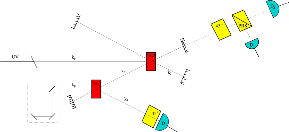
FIG. 1.: Scheme of the experimental apparatus required for the generation and detection of entangled superpositions of macroscopically distinguishable states: The idler beam ($k_{2}$) of the first nonlinear crystal NL1 is used to inject a second nonlinear crystal NL2, while its signal beam ($k_{1}$) triggers the photodetector D₁ after passing through a polarizer. Modes $k_{2}$ and $k_{3}$ are placed within couples of mirrors. The detection apparatus—a rotator, a polarizing beam splitter PBS and the two detectors D_c and D_d—probes the field along $k_{2}$, partially leaking through one of the mirrors of the parametric oscillator.

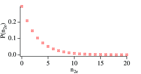
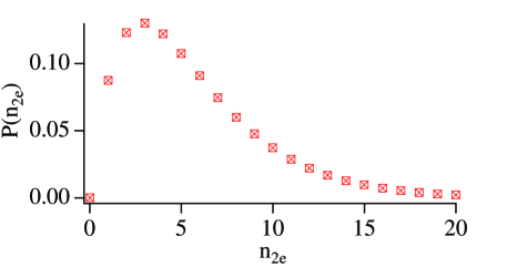
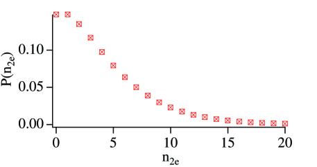
FIG. 2.: Photon-number probability distributions for a photodetection experiment on mode $2e$. $P_{\rm H}(n_{2e})$, $P_{\rm V}(n_{2e})$, and $P(n_{2e})$ [see Eq. (80)] are plotted, respectively, in (a), (b), and (c).

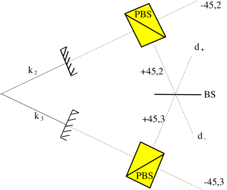
FIG. 3.: Scheme of the experimental arrangement needed for the measurement of the Wigner function (see text). $k_{2}$ and $k_{3}$ represent the cavity modes of Fig. 1

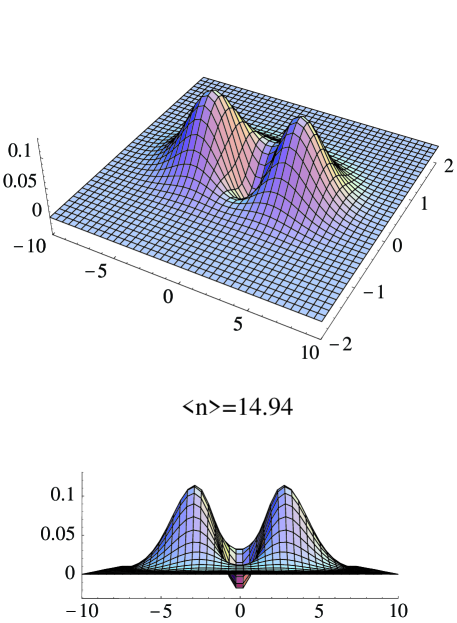
FIG. 4.: Tridimensional plot of the Wigner function for the $d_{+}$ mode for an initial mean number of photons $\langle n\rangle=N=14.94$. Two different viewpoints have been chosen to display more clearly the quantum superposition character of the Schrödinger-cat state.

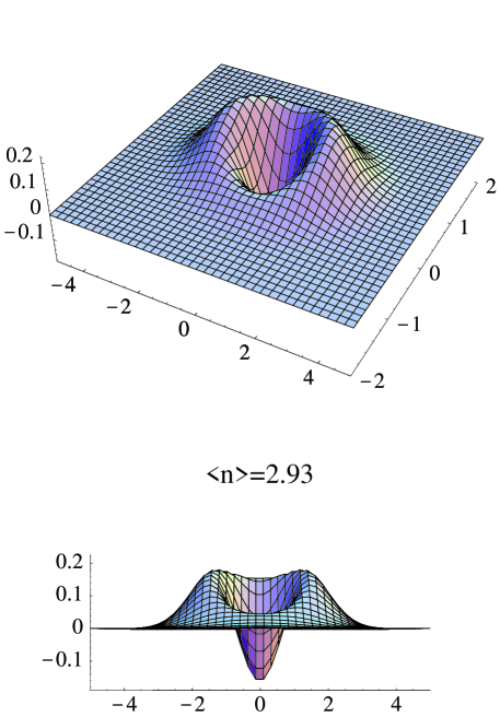
FIG. 5.: Tridimensional plot of the Wigner function for the $d_{+}$ mode for an initial mean number of photons $\langle n\rangle=N=2.93$. In (a) and (b) two different viewpoints have been chosen to display more clearly the quantum superposition character of the Schrödinger-cat state.

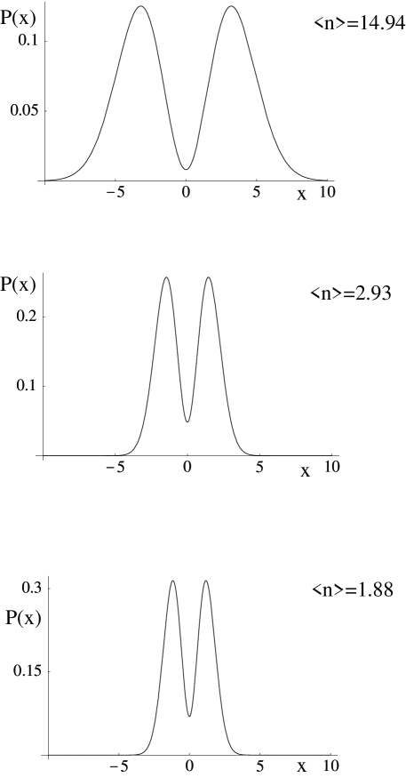
FIG. 6.: Probability distributions $P(x)$ for the quadrature operator $x_{d_{+}}=(d_{+}^{\dagger}+d_{+})/\sqrt{2}$ of the $d_{+}$ mode and for three values of $\langle n\rangle=N$.

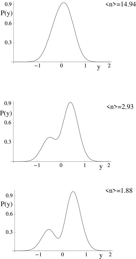
FIG. 7.: Probability distributions $P(y)$ for the quadrature operator $y_{d_{+}}=i(d_{+}^{\dagger}-d_{+})/\sqrt{2}$ of the $d_{+}$ mode and for three values of $\langle n\rangle=N$.

REFERENCES

- [1] Electronic address: mauro@camcat.unicam.it
- [2] E. Schrödinger, Naturwiss. 23, 807 (1935).
- [3] B. Yurke and D. Stoler, Phys. Rev. Lett. 57, 13 (1986). W. Schleich, M. Pernigo, and Fam Le Kien, Phys. Rev. A 44, 2172 (1991).
- [4] W. H. Zurek, Phys. Rev. D 24, 1516 (1981); ibid. 26, 1862 (1982); Phys. Today 44(10), 36 (1991), and references therein.
- [5] M. Brune, E. Hagley, J. Dreyer, X. Maitre, A. Maali, C. Wunderlich, J. M. Raimond and S. Haroche, Phys. Rev. Lett. 77, 4887 (1996).
- [6] S. Habib, K. Shizume, and W. H. Zurek, Phys. Rev. Lett. 80, 4361 (1998).
- [7] C. Monroe, D. M. Meekhof, B. E. King, and D. J. Wineland, Science 272, 1131 (1996).
- [8] E. Schrödinger, Proc. Cambridge Philos. Soc. 31, 555 (1935).
- [9] A. Einstein, B. Podolsky, and N. Rosen, Phys. Rev. 47, 777 (1935).
- [10] C. Bennett, G. Brassard, C. Crépeau, R. Josza, A. Peres, and W. K. Wootters, Phys. Rev. Lett. 70, 1895 (1993). D. Bouwmeester, J.-V. Pan, K. Mattle, M. Eibl, H. Weinfurter, and A. Zeilinger, Nature (London) 390, 575 (1997); D. Boschi, S. Branca, F. De Martini, L. Hardy, and S. Popescu, Phys. Rev. Lett. 80, 1121 (1998).
- [11] A. K. Ekert, Phys. Rev. Lett. 67, 661 (1991); A. K. Ekert et al., ibid. 69, 2881 (1992).
- [12] D. P. DiVincenzo, Science 270, 255 (1995).
- [13] F. De Martini, Phys. Rev. Lett. 81, 2842 (1998); Phys. Lett. A 250, 15 (1998).
- [14] P. G. Kwiat, K. Mattle, H. Weinfurter, A. Zeilinger, A. V. Sergienko, Y. H. Shih, Phys. Rev. Lett. 75, 4337 (1995). For the generation of an ultra-bright source of polarization-entangled photons also see: P. G. Kwiat, E. Waks, A. G. White, I. Appelbaum, and P. H. Eberhard, lanl e-print quant-ph/9810003.
- [15] J. S. Bell, Physics 1, 195 (1964).
- [16] D. M. Greenberger, M. A. Horne, and A. Zeilinger, Am. J. Phys. 58, 1131 (1990); N. D. Mermin, Phys. Rev. Lett. 65, 1838 (1990). D. Bouwmeester et al., to appear (1998).
- [17] M. H. Rubin, D. N. Klyshko, Y. H. Shih, A. V. Sergienko, Phys. Rev. A 50, 5122 (1994).
- [18] L. Davidovich, M. Brune, J. M. Raimond and S. Haroche, Phys. Rev. A 53, 1295 (1996).
- [19] X. Y. Zou, L. J. Wang, L. Mandel, Phys. Rev. Lett. 67, 318 (1991); L. J. Wang, X. Y. Zou, L. Mandel, Phys. Rev. A 44, 4614 (1991); T. P. Grayson, X. Y. Zou, D. Branning, J. R. Torgerson, L. Mandel, Phys. Rev. A 48, 4793 (1993).
- [20] A. O. Caldeira and A. J. Leggett, Phys. Rev. A 31, 1059 (1985); D. F. Walls and G. J. Milburn, Phys. Rev. A 31, 2403 (1985).
- [21] M.O. Scully and M.S. Zubairy, Quantum Optics (Cambridge University Press, Cambridge, 1997). G. J. Milburn and D. F. Walls, Quantum Optics (Springer-Verlag, Berlin, 1994).
- [22] B. Sherman and G. Kurizki, Phys. Rev. A 45, R7674 (1992); B. Sherman, H. Moya-Cessa, P. L. Knight, and G. Kurizki, ibid. 49, 535 (1994). K. Vogel, V. M. Akulin, and W. P. Schleich, Phys. Rev. Lett. 71, 1816 (1993).
- [23] M. Hillery, R. F. O’Connell, M. O. Scully, and E. P. Wigner, Phys. Rep. 106, 121 (1986).
- [24] C. W. Gardiner, Quantum Noise (Springer-Verlag, Berlin,1991).
- [25] H. Risken, The Fokker–Planck Equation (Springer-Verlag, Berlin, 1989).
- [26] G. J. Milburn and D. F. Walls, Quantum Optics (Springer-Verlag, Berlin, 1991).